Diagnostics of Early Faults in Wind Generator Bearings Using Hjorth Parameters

Abstract

Machine learning techniques are a widespread approach to monitoring and diagnosing faults in electrical machines. These techniques extract information from collected signals and classify the health conditions of internal components. Among all internal components, bearings present the highest failure rate. Classifiers commonly employ vibration data acquired from electrical machines, which can indicate different levels of bearing failure severity. Given the circumstances, this work proposes a methodology for detecting early bearing failures in wind turbines, applying classifiers that rely on Hjorth parameters. The Hjorth parameters were applied to analyze vibration signals collected from experiments to distinguish states of normal functioning and states of malfunction, hence enabling the classification of distinct conditions. After the labeling stage using Hjorth parameters, classifiers were employed to provide an automatic early fault identification model, with the decision tree, random forest, support vector machine, and k-nearest neighbors methods presenting accuracy levels of over 95%. Notably, the accuracy of the classifiers was maintained even after undergoing a dimensionality reduction process. Therefore, it can be stated that Hjorth parameters provide a feasible alternative for identifying early faults in wind generators through time-series analysis.

1. Introduction

Due to increased prices during the COVID-19 epidemic, renewable energy production has grown substantially, and the Russian invasion of Ukraine emphasized the energy situation. Between 2023 and 2027, the wind energy market, one of the most representative sources for renewable energy generation, is projected to expand by around 15% annually, increasing by 680 GW of installed capacity, of which 130 GW is expected from offshore plants [1]. In offshore wind farms, which can generate 1.7 times more electricity than commercial wind turbines [2], 25% to 50% of the total generation costs are due to operation and maintenance expenses [3]. Among the components that make up a wind turbine, the generator and electrical system have the highest failure rate, accounting for 35% of failures in offshore wind farms and 25% in onshore wind farms [2].

Electrical machinery is susceptible to mechanical and electrical failures, with mechanical failures accounting for 45–55% and electrical failures accounting for 35–40% of equipment shutdowns [4]. The percentage of failures in electrical machine components was described in [5] as follows: (i) 41% were caused in bearings; (ii) 37% in stators; (iii) 10% in rotors; and (iv) 12% by other issues.

Among all components, the bearing is responsible for the majority of machine failures. According to [4,6], some of the causes of bearing failure are: (i) rotor vibration induced by output torque; (ii) improper assembly; (iii) the deterioration of lubricating fluid; (iv) heat conduction from rotor friction; and (v) friction and contamination.

The bearing is a critical component that supports the shaft of the electrical machine, which plays the role of the generator in wind turbines and is used in other systems, such as transmission and turbine adjustment, supporting large loads and operating in harsh conditions [7]. In response to the high incidence of bearing failure and high-altitude installation, methods for monitoring bearing health conditions have been developed to minimize the expenses associated with maintenance costs and unexpected equipment downtime [8]. Monitoring methods use vibration, acoustic emission, oil analysis, temperature, and other factors to assess failure occurrences [9].

Vibration-based monitoring techniques are reported to be more effective for the identification of mechanical faults [4,10,11], and they can detect changes in component behavior, with vibration signal amplitude representing the severity of the failure [12]. This method is non-invasive because sensors can be installed on the equipment casings to monitor internal components. For example, the internal bearings of a generator can be monitored without the bearing being directly beneath it. However, low-frequency detection issues are limited [3].

Monitoring approaches use signal processing in the time, frequency, or time–frequency domains. Time-domain analysis examines signal variations in a time series using statistical signal information. Frequency-domain analysis examines time series to determine the frequencies present in a given signal. Time–frequency domain analysis combines the two prior techniques, simultaneously analyzing both domains to create a two-dimensional study of the signal [13].

Bearing monitoring and fault detection can be performed using machine learning and domain-specific data. The implemented classification models can either use attributes extracted from the signals along with the class to which the sample belongs, or they can solely utilize the extracted attributes and seek similarity among the samples. The performance of classifiers can be affected by the quantity of data presented to the model, and dimensionality reduction can be implemented to reduce the complexity of the problem, potentially enhancing the classifier performance [14]. In [15], for example, the authors selected optimal signal features for bearing classification through a genetic algorithm and validated the method using the decision tree (DT), random forest (RF), and k-nearest neighbors (k-NN) classifiers. Classification models require a large amount of data for training and validation, which can come from simulation or experimental signals.

Significant studies involving bearing failure have adopted the dataset provided by Case Western Reserve University (CWRU), where bearing failures were introduced through electrical pitting corrosion and signals were already labeled considering the bearing’s health state at the time of data gathering [16,17]. Other studies in the literature have employed bearings with manually inserted faults, as seen in [18,19], where bearing structures were subjected to manual cutting or grinding to collect data.

The dataset provided by the Center for Intelligent Maintenance Systems (IMS) recorded the temporal evolution of vibration signals up to bearing failure without labeling the samples [20]. In this scenario, Hjorth parameters offer a time-domain alternative tool for revealing non-linear and time-varying behavior. They also provide a lower processing complexity than frequency and time–frequency analysis approaches. When just their temporal evolution is available, Hjorth parameters can label vibration signals.

Bo Hjorth [21] created the Hjorth parameters in 1970 to analyze electroencephalogram signals, and they were later applied to rolling vibration signals [22]. Assuming that all subsequent signals acquired were from faults, they proved to be an effective method for estimating the point at which the degeneration of bearings became detectable by the vibration sensor.

Early-stage fault detection is critical due to the high demand for monitoring and detecting problems in electrical machines to prevent unexpected shutdowns. Therefore, this paper proposes a novel method for detecting defects in their early stages. This method analyzes the Hjorth parameters to determine when the bearing fault occurs, allowing the creation of labels for unlabeled datasets and enabling the development of supervised machine learning classification models. The proposed method provides the classifier with time-domain data to detect problems in their earliest stages in wind turbine generator bearings due to the high failure rate and maintenance costs.

Considering the novelty of employing Hjorth’s parameters for fault diagnosis and incorporating features in the time domain, the study is organized as follows. Section 2 explains the methodology proposed for the present study. The experimental dataset used to validate the proposed method is presented in Section 3. The results are discussed in Section 4, and the conclusion is presented in Section 5.

2. Methodology

This study used vibration signals acquired by the Center for Intelligent Maintenance Systems (IMS) at the University of Cincinnati, previously utilized in [20]. Figure 1 depicts the flowchart of the method proposed in this work.

As shown in Figure 1, the method comprised two main stages, with the first one represented by the “Signal separation using Hjorth’s parameters” block, where the analysis was performed using Hjorth’s parameters to determine the time instant at which the fault occurred, allowing the labeling of samples for their use in supervised learning approaches. The second stage, represented by the “Feature engineering and machine learning” block in Figure 1, consisted of extracting time-domain attributes from the signals, as described in Section 2.2, and the quality of these attributes was evaluated. For feature extraction, the implemented classifiers had their hyperparameters tuned through a grid search, aiming to find the topology with the best performance [23]. A dimensionality reduction was also performed to reduce possible noise and redundancy, in an attempt to improve the efficiency of the classifiers [14]. The classifiers were trained with the best identified hyperparameters and features, performance metrics were evaluated, and training and classification time were computed.

2.1. Hjorth’s Parameters

Non-linear bearing degeneration occurs within the time series. Consequently, offline approaches or techniques can be used to detect signal variations. On the other hand, monitoring and failure detection should be performed online, allowing maintenance before bearing collapses.

Bo Hjorth developed the Hjorth parameters in 1970 [21] to evaluate electroencephalogram (EEG) signals, allowing signal analysis to be conducted without the Fourier transform. Since the Hjorth parameters are less complex to compute than the Fourier transform, they can be used for online monitoring and fault detection. The mathematical components of the Hjorth parameters are activity, mobility, and complexity [21].

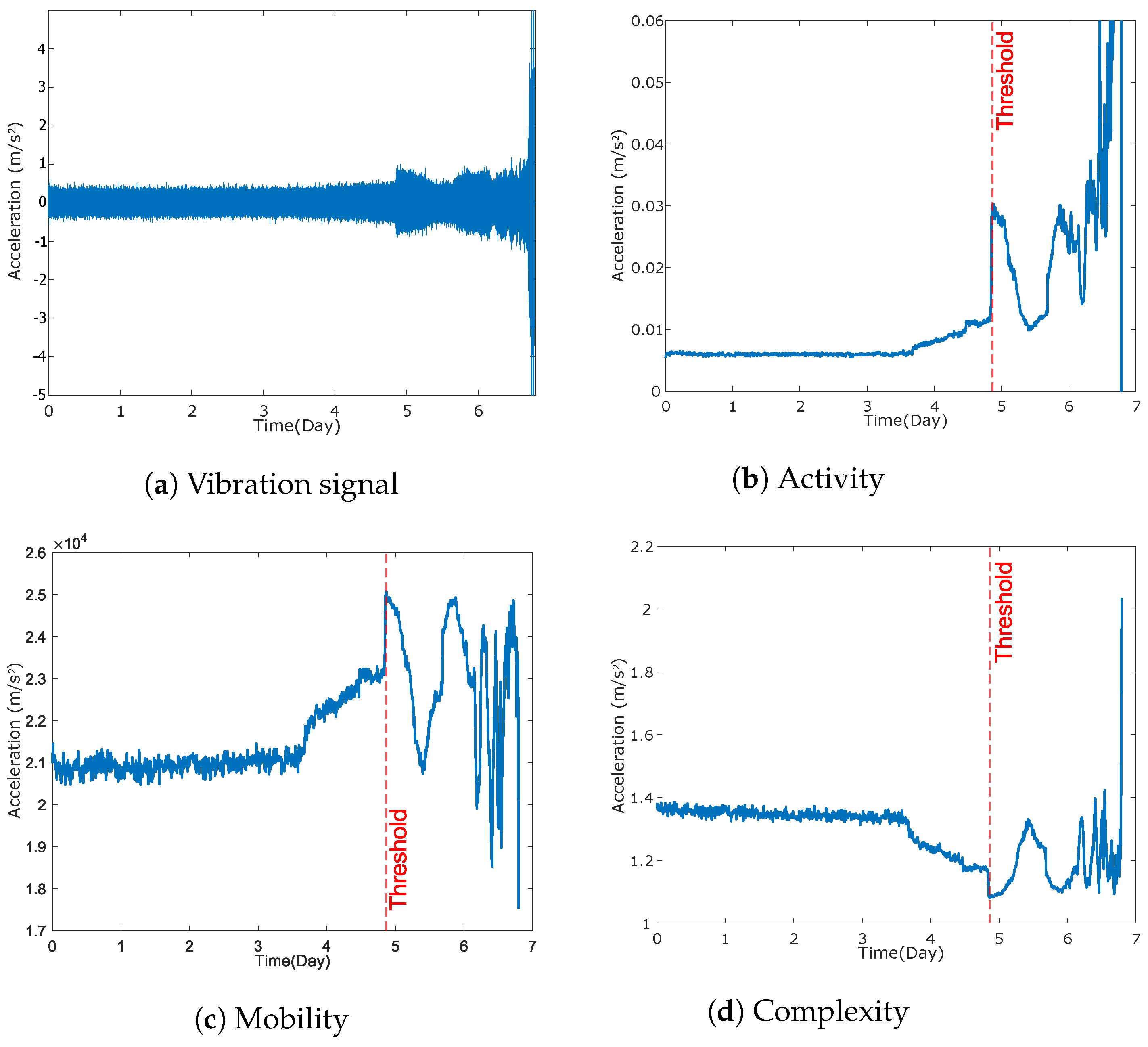
• Activity is defined as the zeroth-order spectral moment ($m_0$), given by Equation (1), and is expressed by the variance (${\sigma }^2$) of the signal amplitude (y), representing the surface envelope of the power spectrum in the time domain.

  $$Activity=m_0={\sigma }^2\left(y\right)$$

  (1)
• Mobility represents the second-order spectral moment ($m_2$), expressed by Equation (2), as the square root of the ratio between the variance (${\sigma }^2$) of the first-order derivative of the signal ($\dot{y}$) and the variance of the signal. A measure of the standard deviation of the slope compared to the standard deviation of the amplitude is established, often known as the mean frequency.

  $$Mobility=m_2=\sqrt{\frac{{\sigma }^2\left(\dot{y}\right)}{{\sigma }^2\left(y\right)}}=\frac{\sigma \left(\dot{y}\right)}{\sigma \left(y\right)}$$

  (2)
  The fact that mobility is a slope measure relative to the mean makes it dependent solely on the waveform shape.
• Complexity is given by the fourth-order spectral moment ($m_4$), defined by Equation (3), as the square root of the ratio between the variance (${\sigma }^2$) of the second-order derivative of the signal amplitude ($\ddot{y}$) and the variance of the first-order derivative of the signal. A measure of the similarity of the waveform under study to a sinusoidal wave is established, expressing a change in the frequency of the analyzed signal.

  $$Complexity=m_4=\sqrt{\frac{{\sigma }^2\left(\ddot{y}\right)}{{\sigma }^2\left(\dot{y}\right)}}$$

  (3)

Using the Hjorth parameters, signal division can be performed by determining the point at which activity and mobility increase suddenly, indicating an increase in signal magnitude and average frequency [22].

The complexity will reduce significantly, reaching close to 1, which indicates that the signal is comparable to a sinusoidal wave. When the Hjorth parameters display the characteristics mentioned above, the point in time represents the border splitting the samples into healthy and faulty ones. Section 4.1 will present the signal separation in more detail.

2.2. Feature Engineering and Machine Learning

The features were calculated from each vibration signal labeled based on the Hjorth parameters related to the motor health status. Each vibration signal from the CWRU dataset was acquired at a sampling rate of 20.48 kHz, with a duration of one second. Each vibration signal and motor health status label comprised an instance of the dataset for training the classifiers. The stages of feature extraction from vibration signals and the classification techniques adopted in this study are presented in this subsection.

2.2.1. Feature Extraction

MATLAB software (R2023a) was used to extract features in the time domain. The following values were extracted from the vibration signals with a duration of 1 s, according to Equations (4) to (13): standard deviation (STD), root mean square (RMS), skewness (SKW), kurtosis, peak value ($V_p$), waveform length (WL), crest factor (CF), factor K (FK), impulse factor (IF), and form factor (FF).

• The standard deviation (STD) is given by Equation (4), where N represents the number of points composing the signal, $\overline{X}$ represents the mean value of the signal amplitude, and $X_i$ is the amplitude of the signal at point i, with the SDT being a measure of data dispersion around the mean value.

  $$STD=\sqrt{\frac{1}{N}\sum _{i=1}^L{|X_i-\overline{X}|}^2}$$

  (4)
• The root mean square (RMS) is expressed by Equation (5), quantifying the average power contained in the signal, serving as a metric for detecting vibration levels yet not being sensitive to early-stage faults.

  $$RMS=\sqrt{\frac{{\sum }_{i=1}^N{X}_i^2}{N}}$$

  (5)
• The skewness (SKW) assesses how far the signal distribution deviates from a normal distribution, and faults can lead to an increase in signal skewness, as expressed by Equation (6).

  $$SKW=\frac{\frac{1}{L}{\sum }_{i=1}^L{|X_i-\overline{X}|}^3}{{\left(\sqrt{\frac{1}{L}{\sum }_{i=1}^L{|X_i-\overline{X}|}^2}\right)}^3}$$

  (6)
• Kurtosis is a measure of the data concentration around the central tendency measures of a normal distribution, given by Equation (7).

  $$Kurtosis=\frac{\frac{1}{L}{\sum }_{i=1}^L{|X_i-\overline{X}|}^4}{{\left(\frac{1}{L}{\sum }_{i=1}^L{|X_i-\overline{X}|}^2\right)}^2}$$

  (7)
• The peak value ($V_p$) checks for the highest absolute value of the signal, given by Equation (8), where X represents the signal amplitude, and an increase in its value may indicate the occurrence of faults.

  $$V_p=\left|max\left(X\right)\right|$$

  (8)
• The waveform length (WL) provides information about the signal frequency, calculated by Equation (9), where P represents the number of signal points and $|x_{i+1}-x_i|$ represents the difference between the amplitude of the current sample i and that of the next sample.

  $$WL=\sum _{i=1}^P|x_{i+1}-x_i|$$

  (9)
• The crest factor (CF) aims to overcome the limitation encountered by the RMS value for sensitivity to early-stage faults, expressed by Equation (10), which is the division of the peak value by the RMS value.

  $$CF=\frac{V_p}{RMS}$$

  (10)
  The peak value has a greater sensitivity to early-stage faults, but as the fault progresses, the RMS value increases faster than the peak value, causing the CF value to decrease in the later stages.
• The factor K (FK) aims to combine the sensitivity of the peak value for early-stage faults and the sensitivity of the RMS value for later-stage fault detection. It is expressed as the product of the two metrics, as in Equation (11).

  $$FK=V_p·RMS$$

  (11)
• The impulse factor (IF) compares the maximum value of the signal to the signal’s mean and is expressed by Equation (12), where $\overline{X}$ represents the signal’s mean value.

  $$IF=\frac{V_p}{\overline{X}}$$

  (12)
• The form factor (FF), given by Equation (13), is defined as the ratio between the RMS value and the mean value of the signal, becoming dependent on the signal’s shape and independent of the signal’s dimensions.

  $$FF=\frac{RMS}{\overline{X}}$$

  (13)

Before being incorporated into the classification models, the above characteristics were subjected to exploratory data analysis to identify absent values.

The parameter ranges varied because of the nature of the calculation and the information they conveyed. Consequently, the data were normalized using min–max normalization [24], depicted in Equation (14), where $X_{max}$ and $X_{min}$ represent the maximum and minimum values from the data, respectively, and $X_i$ represents the value from the data to be normalized. This procedure normalized the parameters to values between 0 and 1, yielding a more accurate representation of the data. The normalized data were used to investigate the correlation between variables and for categorization.

$$X_{i_n}=\frac{X_i-X_{min}}{X_{max}-X_{min}}$$

(14)

2.2.2. Machine Learning

In this work, five machine learning classifiers were employed for the supervised learning of two target classes: healthy and faulty machine conditions. The time-domain features described in Section 2.2.1 were calculated using the Hjorth parameters, and the separation from the Hjorth observation comprised the target feature. The classifiers that were used in this work were:

• Logistic regression (LR) is a statistical method for binary classification that employs input variables to calculate the probability of an event occurring. Utilizing the logistic function to convert values to probabilities ranging from 0 to 1, LR is useful for categorical and binary classification problems [25].
• Decision tree (DT) is a method that predicts outcomes by generating a tree-like structure of decisions based on input features. It divides data into subsets recursively, beginning with the root node, using features that best separate between classes. Leaf nodes represent the result of the predictions. DTs are interpretable, applicable to different fields, and facilitate the hierarchical visualization of decision-making processes [26].
• Random forest (RF) is a DT ensemble-based classification method. Since the decision trees in the RF are generated independently from random samples, there is a low association between the trees. Afterward, voting takes place using the classifications generated by each tree, and the class with the most votes is used to predict the presented sample [27].
• The support vector machine (SVM) algorithm searches for the optimal hyperplane for class separation, and various hyperplanes can be used to divide classes [28]. Nonetheless, the optimal hyperplane is determined by utilizing the most similar samples between the classes, which are the coordinates from which the support vectors are derived. The objective is to maximize distances in both directions to identify the hyperplane with the most significant separation, providing superior generalization [29].
  SVM can classify datasets that are not linearly separable by utilizing a kernel that determines the relationship between higher-dimensional data to identify the separability plane [30].
• The k-nearest neighbors (k-NN) classifier is based on the distance between the new sample to be classified and the other samples. The class of the new sample is determined by the majority class among the nearest neighbors. The parameter k specifies the number of closest points (neighbors) observed during classification, where small k values can lead to less stable results. In contrast, larger k values produce more stable results with increased errors. The Euclidean, Manhattan, or Minkowski functions can compute the distance between points [31].

The hyperparameters of the constructed classification models significantly impacted how each model carried out the learning process and, as a result, its classification performance. Due to the significance of establishing hyperparameters that provided the highest performance, a grid search [32] was utilized to determine the optimal configuration for each implemented classifier by examining a variety of existing hyperparameters.

The number of features presented to a classifier and the hyperparameters immediately affect the classifier’s performance [33]. Depending on the correlation between the variables, insufficient features can hinder the performance of a classifier. In addition, excessive information can result in redundancy or a heightened sensitivity to noises in the model [34].

An increase in the amount of data to be processed increases the computational complexity a model, generates a higher cost in storing these data, and can increase classifier overfitting [34]. Therefore, the feature selection technique was used to identify the most suitable classification features for maintaining or boosting performance levels [14]. Such a process eliminates redundant and irrelevant attributes for classification [34]. The filter-type method, which uses statistical analysis to select the most relevant features, can reduce the feature dimensionality and remove feature similarity, presenting a low computational cost. However, the process is performed without interaction with classifiers, ignoring the dependency between attributes and considering each attribute separately, which can lead to low computational performance [14]. The wrapper approach takes longer to compute than feature selection using filter methods [35]. However, it attempts to discover the ideal subset of data by comparing performance metrics on subsets to determine which combination produces the best performance for the classifier method [34,36].

This study employed a wrapper method with exhaustive feature selection, which assessed all potential combinations of features to identify the subset with the most significant performance metrics.

3. Experimental Setup and Dataset

The vibration signal data were collected experimentally by the Center for IMS at the University of Cincinnati [20]. The experimental setup shown in Figure 2 was realized using 4 Rexnord ZA-2115 double-row roller bearings under a load of 2721.5 kg (6000 lbs), and it can be observed that each bearing had two accelerometers in the x (axial) and y (radial) directions. They were mounted on the shaft connected to an AC motor via belts and maintained at a constant speed of 2000 rpm.

The vibration signal was collected with a 1 s duration for each 10 min interval using integrated circuit piezoelectric (ICP) accelerometers, model PCB 353B33, with a sampling frequency ($f_s$) of 20 kHz. However, in [37], it was shown that the signal was sampled at 20,480 Hz.

An arrangement was employed in which the lubrication of the bearings was forced, causing the lubricating fluid to pass through a tank where a magnetic plug was installed in such a way that debris resulting from bearing degradation was trapped on the plug, preventing it from being re-circulated to the bearings.

The accumulation of a certain amount of debris would lead to the interruption of the experiment. After the experiment was interrupted, the bearings were disassembled, and the bearing that experienced failure and the location of the failure were identified.

The experiment was conducted three times using the same methodology, always starting with new bearings. Among the experiments, Experiment 1 utilized two accelerometers per bearing, positioned in the x and y directions. On the other hand, Experiments 2 and 3 used only one accelerometer per bearing with an unspecified direction.

Table 1. IMS dataset description.

	Quantity of Samples	Bearing Fault	Fault Location
Experiment 1	2156	Bearing 3 Bearing 4	Inner race Roll
Experiment 2	984	Bearing 1	Outer race
Experiment 3	4448	Bearing 3	Outer race

displays the sample quantity, the failed bearing, and the failure location for each experiment.

The bearings exhibited failures after the manufacturer’s specified end-of-life of 100 million revolutions. Bearing 2 did not show any failures in the conducted experiments; therefore, the data from Bearing 2 were not considered.

The data collected during “Experiment 3” were analyzed in [37], where the results were inconsistent. The outer race of “Bearing 3” and the other bearings exhibited no evidence of failure. Therefore, the analysis suggested in this paper did not consider the data from this experiment.

4. Results and Discussion

Due to the fact that the data collected in “Experiment 2” did not specify the direction in which the accelerometer was positioned, they were considered for both the X and Y directions.

4.1. Signal Separation

By applying the Hjorth parameters to the time series of signals obtained from the bearings that failed during the experiments, a threshold for labeling the signals depending on their health condition was established.

The activity ($m_0$) of a signal is directly related to the signal’s average power. Therefore, when the activity suddenly increases, the average power also increases, indicating the occurrence of a failure. Mobility ($m_2$) is correlated with activity, so a sudden increase indicates a failure. Complexity ($m_4$) is a measure of similarity to a sinusoidal wave. When a failure occurs, the parameter temporarily decreases to a value close to 1. Thus, a value of 1 for complexity represents a sinusoidal waveform.

Figure 3 depicts the behavior over time of the vibration signal and Hjorth parameters for the signals collected from the bearing that experienced an outer race fault (Bearing 1—Experiment 2). The vibration signal shown in Figure 3a remained constant until 4.8 days, when an increase in amplitude occurred due to the fault occurrence, and its worsening led to a variation in the acceleration signal. After day 6, approaching the end of the experiment, the high amplitude of the vibration signal was due to the advanced stage of the fault and vibrations transmitted through the shaft from the other bearings.

Figure 3b,c show a similar pattern in terms of activity and mobility, holding a constant value until approximately 3.5 days, when a progressive increase in the parameters began and lasted until 4.8 days. Following this point, there was a sudden rise in amplitude, and the observed variation increased dramatically. Another point to highlight is the fact that the activity was related to the power of the vibration signal, and it exhibited a behavior in response to the signal. Meanwhile, the mobility showed a significant variation after the fault occurrence but did not follow the increase in vibrations in the final moments of the test, as it is a measure of the signal’s average frequency.

Figure 3d shows that the complexity began to decline at 3.8 days, and the minimum value was attained at 4.8 days after a rapid decrease in the parameter, approaching similarity to a sine wave in the time domain, indicating the occurrence of bearing failure. The increase in activity and mobility associated with the moment when the complexity reached its minimum value indicated bearing failure, with day 4.8 being the moment used to establish the separability threshold of the signals.

The established threshold for labeling the samples enabled the presentation of faulty samples from the early stages of failure, making the classifier capable of classifying the health condition at different stages of failure, thereby increasing its generalization power.

Another analysis enabled by the Hjorth parameters was the observation of the pre-failure moment, which occurred between days 3.8 and 4.8, where the parameter variations began. Such behavior could not be observed solely from the vibration signal.

The preceding analysis was applied to the data from Bearings 3 and 4 of “Experiment 1”, and MATLAB software was used to determine the instant when a sudden increase in the average power (activity) and average frequency (mobility) of the signal occurred, as well as the instant when the signal’s resemblance to a sinusoidal wave (complexity) reached its minimum value, close to 1. The day of the occurrence of failure for each bearing in its respective experiment, as well as the quantity of healthy and failed samples, is shown in

Table 2. Treshold of the faults.

	Day of Fault	Number of Healthy Samples	Number of Faulty Samples
Bearing 3—Experiment 1	33	1910	246
Bearing 4—Experiment 1	25	1540	616
Bearing 1—Experiment 2	4.8	704	280

.

The bearings exhibited failures in different structural locations. To achieve increased generalization power for the classifiers, samples from all bearings were merged, resulting in 4154 healthy signals and 1142 faulty signals. After separating the signals, the attributes STD, RMS, SKW, kurtosis, $V_p$, WL, CF, FK, IF, and FF, presented in Section 2.2.1, were extracted from the vibration signal.

4.2. Classification

The classifiers conducted a grid search in pursuit of the best hyperparameters before the data were presented for the training and validation process.

Table 3. Hyperparameters adjusted using grid search.

Classifier	Hyperparameter	Tested Values	Selected
LR	C	0.2, 2, 20, 80	0.2
	Penalty	L2, Elasticnet	L2
	Solver	lbfgs, liblinear, sag, saga	lbfgs
DT	Criterion	Gini, Entropy	Entropy
	Tree depth	1, 2, 3, 4, 5, 6, 7, 8, 9, 10	10
	Data points to split a node	8, 10, 12	10
	Tree depth	10, 20, 30	10
	Attributes to split a node	2, 3	3
RF	Data points to split a node	8, 10, 12	10
	Minimum allowed data in a leaf	3, 4, 5	3
	Number of trees	100, 150, 200, 250	100
	C	0.1, 5, 10, 20, 50	50
SVM	Kernel coefficient	0.001, 0.01, 0.1, 1	1
	Kernel	RBF, Linear	RBF
k-NN	Number of neighbors (k)	3, 5, 7, 9, 11	11
	Weights	Uniform, Distance	Distance
	Metric	Minkowski, Euclidian, Manhattan	Minkowski

displays the set of tested hyperparameters and those selected for constructing each classifier.

The datasets were divided in an 80/20 stratified ratio and presented to the three classifiers with the selected hyperparameters shown in Table 3. The accuracy, precision, recall, F1 score, and time taken for model training and classification were examined.

Table 4. Performance metrics according to the x-axis and all features.

	Classifier
Metric	LR	DT	RF	SVM	$\mathit{k}$-NN
Accuracy	0.82	0.98	0.99	0.97	0.98
Precision	0.85	0.98	0.98	0.97	0.98
Recall	0.58	0.96	0.98	0.94	0.96
F1 score	0.59	0.97	0.98	0.95	0.97
$T_{train}\left(s\right)$	2.54	3.98	122.64	25.62	0.73
$T_{test}\left(s\right)$	0.0007	0.001	0.015	0.072	0.011

and

Table 5. Performance metrics according to the x-axis and all features.

	Classifier
Metric	LR	DT	RF	SVM	$\mathit{k}$-NN
Accuracy	0.84	0.99	0.99	0.97	0.99
Precision	0.91	0.98	0.99	0.97	0.98
Recall	0.61	0.98	0.99	0.94	0.98
F1 score	0.63	0.98	0.99	0.96	0.98
$T_{train}\left(s\right)$	2.49	3.38	105.05	22.41	0.73
$T_{test}\left(s\right)$	0.0019	0.0022	0.023	0.051	0.012

present the metrics obtained for the x and y directions.

The classifiers did not show significant variations among themselves when considering performance metrics. However, for data from the y-axis, the recall was higher for RF and k-NN, indicating a lower occurrence of false negatives, and the time taken for classification was shorter for all classifiers when compared to the data from the x-axis.

The dimensionality reduction approach was utilized to decrease the initial problem of 10 features to 2 using the wrapper method of exhaustive feature selection (EFS). When EFS is applied to the number of features, the amount of data to be processed and stored decreases by 80%. The EFS technique executes the search by assessing all feasible subsets and returning the best attribute combination.

Table 6. Remaining features after feature selection.

Classifier	Features
LR	STD and $V_p$
DT	WL and FF
RF	RMS and WL
SVM	STD and WL
k-NN	RMS and WL

presents the selected subsets for each classifier using an exhaustive attribute search.

The subset formed by the selected attributes after dimensionality reduction was once again divided in an 80/20 stratified ratio and applied to the classifiers.

Table 7. Performance metrics according to the x-axis regarding the two remaining features. The values in parentheses represent the difference between the entire set and the remaining features.

	Classifier
Metric	LR	DT	RF	SVM	k-NN
Accuracy	0.82 ($-0\%$)	0.98 ($-0\%$)	0.98 ($\downarrow 1\%$)	0.96 ($\downarrow 1\%$)	0.98 ($\downarrow 1\%$)
Precision	0.86 ($\uparrow 1\%$)	0.97 ($\downarrow 1\%$)	0.98 ($-0\%$)	0.96 ($\downarrow 1\%$)	0.97 ($\downarrow 1\%$)
Recall	0.56 ($\downarrow 2\%$)	0.96 ($-0\%$)	0.97 ($\downarrow 1\%$)	0.92 ($\downarrow 2\%$)	0.97 ($\uparrow 1\%$)
F1 score	0.56 ($\downarrow 3\%$)	0.97 ($-0\%$)	0.97 ($\downarrow 1\%$)	0.94 ($\downarrow 1\%$)	0.97 ($-0\%$)
$T_{train}\left(s\right)$	0.77 ($\Downarrow 69\%$)	1.21 ($\Downarrow 51\%$)	89.52 ($\Downarrow 27\%$)	24.33 ($\Downarrow 5\%$)	0.51 ($\Downarrow 30\%$)
$T_{test}\left(s\right)$	0.001 ($\Downarrow 42\%$)	0.002 ($\Uparrow 50\%$)	0.018 ($\Uparrow 20\%$)	0.065 ($\Downarrow 10\%$)	0.004 ($\Downarrow 64\%$)

and

Table 8. Performance metrics according to the y-axis regarding the two remaining features. The values in parentheses represent the difference between the entire set and the remaining features.

	Classifier
Metric	LR	DT	RF	SVM	k-NN
Accuracy	0.82 ($\downarrow 2\%$)	0.98 ($\downarrow 1\%$)	0.99 ($-0\%$)	0.96 ($\downarrow 1\%$)	0.98 ($\downarrow 1\%$)
Precision	0.91 ($-0\%$)	0.98 ($-0\%$)	0.98 ($\downarrow 1\%$)	0.96 ($\downarrow 1\%$)	0.98 ($-0\%$)
Recall	0.57 ($\downarrow 4\%$)	0.97 ($\downarrow 1\%$)	0.98 ($\downarrow 1\%$)	0.93 ($\downarrow 1\%$)	0.97 ($\downarrow 1\%$)
F1 score	0.58 ($\downarrow 5\%$)	0.97 ($\downarrow 1\%$)	0.98 ($\downarrow 1\%$)	0.94 ($\downarrow 2\%$)	0.98 ($-0\%$)
$T_{train}\left(s\right)$	0.81 ($\Downarrow 67\%$)	1.24 ($\Downarrow 63\%$)	86.14 ($\Downarrow 18\%$)	24.39 (⇑ 4.8%)	0.53 (⇓ 27.4%)
$T_{test}\left(s\right)$	0.001 ($\Downarrow 36\%$)	0.002 ($\Downarrow 22\%$)	0.025 ($\Uparrow 25\%$)	0.060 ($\Uparrow 20\%$)	0.004 (⇓ 55.5%)

present the performance metrics and the variation compared to the complete dataset.

The classifiers showed a small reduction of 1% for almost all observed performance metrics, and RF and k-NN exhibited significant reductions in the time required for classifier training, while SVM required more time. Variation in the time required to classify the samples after training was also observed, although with millisecond-scale differences.

Sample dispersion could be visualized due to the dimensionality reduction to only two variables. Figure 4 depicts the scatter plot of samples for both axes, representing the two subsets generated in the dimensionality reduction process. Figure 4a,b depict the data dispersion between WL and RMS used by the RF and k-NN classifiers. In these figures, a region is visible where healthy and faulty samples mix, but due to the adjusted hyperparameters, the classifiers achieved an accuracy of 98%. Figure 4c,d display the dispersion between STD and WL, used by the SVM classifier. In this case, a region of overlap between the classes is observed, and even with adjusted hyperparameters, the classifier could not match the performance achieved by the RF and k-NN classifiers.

Figure 4e,f depict the data dispersion between the WL and factor form, which were selected by the DT classifier. Despite being a classifier with lower complexity than RF, SVM, and k-NN, the data showed a small overlap region between the samples.

The dispersion between STD and $V_p$ used by logistic regression (LR), as shown in Figure 4g,h, exhibited a significant overlap region between healthy and faulty samples. Due to its simpler nature, this classifier yielded the lowest performance metrics among all implemented classifiers.

All subsets exhibited a region of sample concentration for both healthy and faulty cases, which could confuse the classifiers. These regions may help to explain the increased training time, as the SVM method sought a separating hyperplane. The confusion region could be explained by the similarity of the signals in the threshold of healthy and faulty samples separated by the Hjorth parameters.

4.3. Comparative Analysis

The efficacy of classifiers utilizing the method provided in this paper was compared to previous works that used the same dataset. The classifier chosen for the comparison was k-NN, since its performance metrics were comparable to those of RF, which had the highest performance metrics, and the computing time needed for training and classification was the lowest among the classifier models employed.

Table 9. Comparison of results for the same dataset based on other methods. The abbreviations are as follows: wavelet packet decomposition (WPD), support tensor data description (STDD), k-nearest neighbor (KNN), entropy-based combined indicator (COM), grasshopper optimization algorithm (GOA), support vector data description (SVDD), generalized multiscale Poincare plots (GMPOP), cyclic spectral correlation (CSC), support vector data description with negative sample (NSVDD).

Method	Accuracy	Precision	Recall	F1 Score
Our approach	0.98	0.98	0.97	0.98
WPD-STDD [38]	1.00	1.00	–	–
KNN [38]	0.97	0.97	–	–
COM-GOA-SVDD [39]	0.92	0.90	1.00	0.94
GMPOP [40]	0.99	–	1.00	–
CSC—NSVDD [41]	0.99	0.99	0.99	0.99

shows the performance indicators obtained by other approaches used in other research efforts. The symbol “–” indicates that the study did not provide the observed metric.

The best performance achieved by the methods in the literature was attained in [38]. However, the models were trained using equal quantities of healthy and faulty samples, even though these machines spend most of their time operating under normal conditions. The works [38,39,40,41] applied their respective methodologies using only the data collected in Experiment 2, which consisted solely of faulty signals from the outer race, in contrast to the method presented in this study. Our approach utilized data collected from Experiments 1 and 2, enabling the classifier to receive faulty data from the inner race, outer race, and rolling elements.

The method with the best metrics was WPD—STDD, implemented in [38], which achieved an accuracy and precision of 100%. However, it is a tensor-based method that also uses attributes extracted in both the time and frequency domains, making it a computationally more expensive method with higher data storage requirements than that presented in this article, which solely utilized attributes in the time domain.

Another method with superior metrics to that proposed in this article was presented in [40], achieving an accuracy of 99%. However, the method was trained using only healthy samples with the non-linear dynamics of the bearing for the detection of early-stage faults. Nevertheless, since the model uses only healthy samples, it may be biased.

The proposed method presents the advantage of obtaining characteristic information and performing the analysis of vibration signals using attributes extracted directly in the time domain without applying transforms to the frequency domain. The attributes required for monitoring and diagnosing the bearings do not present complexity in their calculation, enabling online monitoring.

The proposed method exhibited good performance in classifying the samples. However, a limitation arises from its requirement of a historical series, from the start of operation until the equipment stops due to bearing failure, as it is dependent on signals that exhibit failure and demands the processing of a large amount of data.

5. Conclusions

The Hjorth parameters proved to be an effective method for determining the instance within a time series that separates healthy signals and faulty signals, allowing the labeling of each sample for use in supervised learning classifiers without the need for frequency-domain analysis.

The information extracted from the time-domain vibration signals, combined with the classes resulting from the separation based on the Hjorth parameters and adjustments to the internal structure of the classifiers, made it possible to achieve an accuracy exceeding 95% for the four implemented classifiers.

The dimensionality reduction demonstrated that by using only 2 attributes, it was possible to maintain a performance level similar to classifiers trained using the original 10 attributes. The DT, RF, k-NN, LR, and SVM models used the WL attribute after the dimensionality reduction process, showing it to be an attribute that carries relevant information, as it can be considered a measure of signal frequency.

The best results were found when analyzing the signals from the y-axis, which may indicate that the accelerometers used in Experiments 2 and 3 were positioned in the y-direction, and the similarity between the results presented in Table 7 and Table 8 indicated the need for only one accelerometer sensor for monitoring and fault detection, preferably positioned in the y-axis direction.

Future work will involve applying the proposed method to address multiclass classification problems, identifying the location of bearing faults, whether it be the inner race, outer race, or rolling elements. This analysis has the potential to facilitate the identification of the fundamental cause of the failure and to verify the classifier’s performance for ball bearings, which are commonly used in electric motors.

References

1. Hutchinson, M.; Zhao, F. GWEC Global Wind Report; Hutchinson, M., Zhao, F., Eds.; GWEC: Brussels, Belgium, 2023. [Google Scholar]
2. Attallah, O.; Ibrahim, R.A.; Zakzouk, N.E. CAD system for inter-turn fault diagnosis of offshore wind turbines via multi-CNNs & feature selection. Renew. Energy 2023, 203, 870–880. [Google Scholar] [CrossRef]
3. Badihi, H.; Zhang, Y.; Jiang, B.; Pillay, P.; Rakheja, S. A Comprehensive Review on Signal-Based and Model-Based Condition Monitoring of Wind Turbines: Fault Diagnosis and Lifetime Prognosis. Proc. IEEE 2022, 110, 754–806. [Google Scholar] [CrossRef]
4. Gangsar, P.; Tiwari, R. Signal based condition monitoring techniques for fault detection and diagnosis of induction motors: A state-of-the-art review. Mech. Syst. Signal Process. 2020, 144, 106908. [Google Scholar] [CrossRef]
5. Vaimann, T.; Belahcen, A.; Kallaste, A. Necessity for implementation of inverse problem theory in electric machine fault diagnosis. In Proceedings of the IEEE International Symposium on Diagnostics for Electrical Machines, Power Electronics and Drives (SDEMPED), Guarda, Portugal, 1–4 September 2015; pp. 380–385. [Google Scholar] [CrossRef]
6. Spyropoulos, D.V.; Mitronikas, E.D. A Review on the Faults of Electric Machines Used in Electric Ships. Adv. Power Electron. 2013, 2013, 216870. [Google Scholar] [CrossRef]
7. Liu, Z.; Zhang, L. A review of failure modes, condition monitoring and fault diagnosis methods for large-scale wind turbine bearings. Measurement 2020, 149, 107002. [Google Scholar] [CrossRef]
8. Nabhan, A.; Ghazaly, N.; Samy, A.; Mousa, M.O. Bearing Fault Detection Techniques—A Review. Turk. J. Eng. Sci. Technol. 2015, 3. [Google Scholar]
9. Duan, Z.; Wu, T.; Guo, S.; Shao, T.; Malekian, R.; Li, Z. Development and trend of condition monitoring and fault diagnosis of multi-sensors information fusion for rolling bearings: A review. Int. J. Adv. Manuf. Technol. 2018, 96, 803–819. [Google Scholar] [CrossRef]
10. Gundewar, S.K.; Kane, P.V. Condition Monitoring and Fault Diagnosis of Induction Motor. J. Vib. Eng. Technol. 2021, 9, 643–674. [Google Scholar] [CrossRef]
11. Tama, B.A.; Vania, M.; Lee, S.; Lim, S. Recent advances in the application of deep learning for fault diagnosis of rotating machinery using vibration signals. Artif. Intell. Rev. 2023, 56, 4667–4709. [Google Scholar] [CrossRef]
12. Gnanasekaran, S.; Jakkamputi, L.; Thangamuthu, M.; Marikkannan, S.K.; Rakkiyannan, J.; Thangavelu, K.; Kotha, G. Condition Monitoring of an All-Terrain Vehicle Gear Train Assembly Using Deep Learning Algorithms with Vibration Signals. Appl. Sci. 2022, 12, 10917. [Google Scholar] [CrossRef]
13. KiranKumar, M.V.; Lokesha, M.; Kumar, S.; Kumar, A. Review on Condition Monitoring of Bearings using vibration analysis techniques. IOP Conf. Ser. Mater. Sci. Eng. 2018, 376, 012110. [Google Scholar] [CrossRef]
14. Souza, W.A.; Alonso, A.M.; Bosco, T.B.; Garcia, F.D.; Gonçalves, F.A.; Marafão, F.P. Selection of features from power theories to compose NILM datasets. Adv. Eng. Inform. 2022, 52, 101556. [Google Scholar] [CrossRef]
15. Toma, R.N.; Prosvirin, A.E.; Kim, J.M. Bearing Fault Diagnosis of Induction Motors Using a Genetic Algorithm and Machine Learning Classifiers. Sensors 2020, 20, 1884. [Google Scholar] [CrossRef] [PubMed]
16. Neupane, D.; Seok, J. Bearing Fault Detection and Diagnosis Using Case Western Reserve University Dataset with Deep Learning Approaches: A Review. IEEE Access 2020, 8, 93155–93178. [Google Scholar] [CrossRef]
17. Wang, H.; Yue, W.; Wen, S.; Xu, X.; Haasis, H.D.; Su, M.; Liu, P.; Zhang, S.; Du, P. An improved bearing fault detection strategy based on artificial bee colony algorithm. CAAI Trans. Intell. Technol. 2022, 7, 570–581. [Google Scholar] [CrossRef]
18. Pacheco-Chérrez, J.; Fortoul-Díaz, J.A.; Cortés-Santacruz, F.; María Aloso-Valerdi, L.; Ibarra-Zarate, D.I. Bearing fault detection with vibration and acoustic signals: Comparison among different machine leaning classification methods. Eng. Fail. Anal. 2022, 139, 106515. [Google Scholar] [CrossRef]
19. Shen, S.; Lu, H.; Sadoughi, M.; Hu, C.; Nemani, V.; Thelen, A.; Webster, K.; Darr, M.; Sidon, J.; Kenny, S. A physics-informed deep learning approach for bearing fault detection. Eng. Appl. Artif. Intell. 2021, 103, 104295. [Google Scholar] [CrossRef]
20. Qiu, H.; Lee, J.; Lin, J.; Yu, G. Wavelet filter-based weak signature detection method and its application on rolling element bearing prognostics. J. Sound Vib. 2006, 289, 1066–1090. [Google Scholar] [CrossRef]
21. Hjorth, B. EEG analysis based on time domain properties. Electroencephalogr. Clin. Neurophysiol. 1970, 29, 306–310. [Google Scholar] [CrossRef]
22. Jacopo, C.C.M.; Matteo, S.; Riccardo, R.; Marco, C. Analysis of NASA Bearing Dataset of the University of Cincinnati by Means of Hjorth’s Parameters. In Archivio Istituzionale della Ricerca; Università di Modena e Reggio Emilia: Reggio Emilia, Italy, 2018. [Google Scholar]
23. Vitor, A.L.; Goedtel, A.; Barbon, S.; Bazan, G.H.; Castoldi, M.F.; Souza, W.A. Induction motor short circuit diagnosis and interpretation under voltage unbalance and load variation conditions. Expert Syst. Appl. 2023, 224, 119998. [Google Scholar] [CrossRef]
24. Mazziotta, M.; Pareto, A. Normalization methods for spatio-temporal analysis of environmental performance: Revisiting the Min–Max method. Environmetrics 2022, 33, e2730. [Google Scholar] [CrossRef]
25. Tsangaratos, P.; Ilia, I. Comparison of a logistic regression and Naïve Bayes classifier in landslide susceptibility assessments: The influence of models complexity and training dataset size. CATENA 2016, 145, 164–179. [Google Scholar] [CrossRef]
26. Souza, W.A.; Marafão, F.P.; Liberado, E.V.; Simões, M.G.; Da Silva, L.C.P. A NILM Dataset for Cognitive Meters Based on Conservative Power Theory and Pattern Recognition Techniques. J. Control Autom. Electr. Syst. 2018, 29, 742–755. [Google Scholar] [CrossRef]
27. Saravanan, S.; Reddy, N.M.; Pham, Q.B.; Alodah, A.; Abdo, H.G.; Almohamad, H.; Al Dughairi, A.A. Machine Learning Approaches for Streamflow Modeling in the Godavari Basin with CMIP6 Dataset. Sustainability 2023, 15, 12295. [Google Scholar] [CrossRef]
28. Guenther, N.; Schonlau, M. Support Vector Machines. Stata J. Promot. Commun. Stat. Stata 2016, 16, 917–937. [Google Scholar] [CrossRef]
29. Jiang, P.; Li, R.; Liu, N.; Gao, Y. A novel composite electricity demand forecasting framework by data processing and optimized support vector machine. Appl. Energy 2020, 260, 114243. [Google Scholar] [CrossRef]
30. Chowdhury, S.; Schoen, M.P. Research Paper Classification using Supervised Machine Learning Techniques. In Proceedings of the 2020 Intermountain Engineering, Technology and Computing (IETC), Orem, UT, USA, 2–3 October 2020; pp. 1–6. [Google Scholar] [CrossRef]
31. Yesilbudak, M.; Ozcan, A. kNN Classifier Applications in Wind and Solar Energy Systems. In Proceedings of the 2022 11th International Conference on Renewable Energy Research and Application (ICRERA), Istanbul, Turkey, 18–21 September 2022; pp. 480–484. [Google Scholar] [CrossRef]
32. Fayed, H.A.; Atiya, A.F. Speed up grid-search for parameter selection of support vector machines. Appl. Soft Comput. 2019, 80, 202–210. [Google Scholar] [CrossRef]
33. Mantovani, R.G.; Rossi, A.L.; Alcobaça, E.; Vanschoren, J.; de Carvalho, A.C. A meta-learning recommender system for hyperparameter tuning: Predicting when tuning improves SVM classifiers. Inf. Sci. 2019, 501, 193–221. [Google Scholar] [CrossRef]
34. Venkatesh, B.; Anuradha, J. A Review of Feature Selection and Its Methods. Cybern. Inf. Technol. 2019, 19, 3–26. [Google Scholar] [CrossRef]
35. Got, A.; Moussaoui, A.; Zouache, D. Hybrid filter-wrapper feature selection using whale optimization algorithm: A multi-objective approach. Expert Syst. Appl. 2021, 183, 115312. [Google Scholar] [CrossRef]
36. Sathianarayanan, B.; Singh Samant, Y.C.; Conjeepuram Guruprasad, P.S.; Hariharan, V.B.; Manickam, N.D. Feature-based augmentation and classification for tabular data. CAAI Trans. Intell. Technol. 2022, 7, 481–491. [Google Scholar] [CrossRef]
37. Gousseau, W.; Antoni, J.; Girardin, F.; Griffaton, J. Analysis of the Rolling Element Bearing data set of the Center for Intelligent Maintenance Systems of the University of Cincinnati. In Proceedings of the CM2016, Charenton, France, 10–12 October 2016. [Google Scholar]
38. Sun, B.; Liu, X. Bearing early fault detection and degradation tracking based on support tensor data description with feature tensor. Appl. Acoust. 2022, 188, 108530. [Google Scholar] [CrossRef]
39. Zhang, J.; Zhang, Q.; Qin, X.; Sun, Y. A two-stage fault diagnosis methodology for rotating machinery combining optimized support vector data description and optimized support vector machine. Measurement 2022, 200, 111651. [Google Scholar] [CrossRef]
40. Shao, K.; He, Y.; Xing, Z.; Du, B. Detecting wind turbine anomalies using nonlinear dynamic parameters-assisted machine learning with normal samples. Reliab. Eng. Syst. Saf. 2023, 233, 109092. [Google Scholar] [CrossRef]
41. Liu, C.; Gryllias, K. A semi-supervised Support Vector Data Description-based fault detection method for rolling element bearings based on cyclic spectral analysis. Mech. Syst. Signal Process. 2020, 140, 106682. [Google Scholar] [CrossRef]
Figure 1. Flowchart of the methodology.
Sustainability 15 14673 g001
Figure 2. Experimental setup of the IMS.
Sustainability 15 14673 g002
Figure 3. Hjorth parameters analysis and separation threshold between healthy and faulty condition.
Sustainability 15 14673 g003
Figure 4. Dispersion of samples for the subsets. (a) WL and RMS of the signal on the x-axis. (b) WL and RMS of the signal on the y-axis. (c) STD and RMS of the signal on the x-axis. (d) STD and RMS of the signal on the y-axis. (e) WL and FF of the signal on the x-axis. (f) WL and FF of the signal on the y-axis. (g) STD and V p of the signal on the x-axis. (h) STD and V p of the signal on the y-axis.
Sustainability 15 14673 g004