An Artificial Intelligence-Based Stacked Ensemble Approach for Prediction of Protein Subcellular Localization in Confocal Microscopy Images

Abstract

Predicting subcellular protein localization has become a popular topic due to its utility in understanding disease mechanisms and developing innovative drugs. With the rapid advancement of automated microscopic imaging technology, approaches using bio-images for protein subcellular localization have gained a lot of interest. The Human Protein Atlas (HPA) project is a macro-initiative that aims to map the human proteome utilizing antibody-based proteomics and related c. Millions of images have been tagged with single or multiple labels in the HPA database. However, fewer techniques for predicting the location of proteins have been devised, with the majority of them relying on automatic single-label classification. As a result, there is a need for an automatic and sustainable system capable of multi-label classification of the HPA database. Deep learning presents a potential option for automatic labeling of protein’s subcellular localization, given the vast image number generated by high-content microscopy and the fact that manual labeling is both time-consuming and error-prone. Hence, this research aims to use an ensemble technique for the improvement in the performance of existing state-of-art convolutional neural networks and pretrained models were applied; finally, a stacked ensemble-based deep learning model was presented, which delivers a more reliable and robust classifier. The F1-score, precision, and recall have been used for the evaluation of the proposed model’s efficiency. In addition, a comparison of existing deep learning approaches has been conducted with respect to the proposed method. The results show the proposed ensemble strategy performed exponentially well on the multi-label classification of Human Protein Atlas images, with recall, precision, and F1-score of 0.70, 0.72, and 0.71, respectively.

1. Introduction

Plasma membranes encase all eukaryotic cells, containing complicated organelles and a complex endomembrane system. Different compartments for varied metabolic activities are provided by these organelles. Only one of these organelles, the cytosol, can synthesize proteins. From the cytosol, these proteins are then transported to their target destination organelle to perform their functions. Protein translocation is required for proteins to function in multiple organelles. To approach their functional destination, almost 50% of a cell’s proteins must be carried inside or across at least one cell membrane. Subcellular localization refers to the position of a protein within cellular compartments. For protein function, subcellular localization has been proposed to increase functional diversity while minimizing the cost of designing and synthesizing proteins [1]. It also controls protein interaction with other proteins and the posttranslational modification machinery, allowing proteins to be integrated into biological networks. Human disorders, such as cancer, kidney stones, and neurogenerative conditions like Alzheimer’s disease, have been related to abnormally localized proteins [2].

A lot of data is needed to be acquired regarding subcellular protein distributions and how they vary throughout cell populations to comprehend the complicated mechanisms that control biological processes at the cellular level. Automatic recognition of fluorescence microscopy images is an excellent tool for obtaining this data [3]. High temporal and spatial resolution imaging of living cells is possible thanks to fluorescent probes’ high specificity for tagging elements of interest and the accessibility of modern fluorescence microscopes. Furthermore, understanding the chemical pathways that underpin cell functions requires correct protein localization.

The HPA project is currently working on annotating the localization of human proteins inside cells using biotechnology [4]. HPA uses fluorescence-based microscopy techniques to capture images [3]. For mapping the expression of the human proteome, researchers used a systematic antibody-based technique to create trillions of fluorescence microscopy images [5]. These data can reveal necessary information about cellular processes and biochemical pathways unless we can overcome the obstacles of analyzing such a large quantity of images.

In the recent past, with rapid technological improvement and a wide range of applications, Artificial Intelligence has become increasingly prevalent due to its robust applicability in situations that cannot be solved well by humans or traditional computing structures. Artificial intelligence with deep learning and machine learning is having a significant impact in all industries, including agriculture [6,7,8], medical diagnostics [9], education [10], autonomous vehicles [11], voice assistants [12], and many more.

Researchers have recently proposed techniques combining fluorescence microscopy with machine learning and deep learning methods to predict protein subcellular localization. Due to the vast quantity of high-resolution microscopic images collected, it is now possible to build high-performance identification and classification systems using deep neural network-based methods. Protein localization using microscopic images, on the other hand, poses a distinct machine learning difficulty, namely, how to cope with data that are poorly annotated. The problem is that instead of labeling individual incidents, a collection of them has been labeled (in this case, cells). Each of these instances could provide insight into the correct classification. As a result, this is a multi-label classification problem, which means that an image could have multiple labels associated with it.

There are numerous approaches to tackle multi-label classification issues [13,14,15] and these approaches can be categorized as algorithm adaptation method and problem transformation method [16]. The first category includes algorithms like Rank-SVM [17], ML-DT [18], and ML-KNN [19], which can be extended to process multi-label data. In the second situation, a multi-label classification problem is broken down into several single-label classification problems, or even one multi-class classification problem. Classifier chains [20,21,22], Label Powerset [23], and Binary Relevance [24,25] are examples of this type of technique. There are still challenges with the aforesaid algorithms in real-world applications, such as class imbalance, label correlations, and high dimensionality.

Furthermore, some ensemble techniques have been presented as benchmarks for multi-label classification tasks in recent years [26,27]. However, all existing models usually consider the bagging concept in order to build a variety of ensemble classifier models and finally use majority voting to merge them for the final outcome. Another prominent method is the stacked ensembled technique, which has been demonstrated to be beneficial to a variety of learning tasks. A stacked ensemble has been developed in this study, which uses pretrained models as ensemble members and has been fine-tuned on the HPA dataset. We anticipate that the suggested approach can be used for a better understanding of an automated classification method for the multi-label HPA problem. Following are the contributions made by the author in this research work:

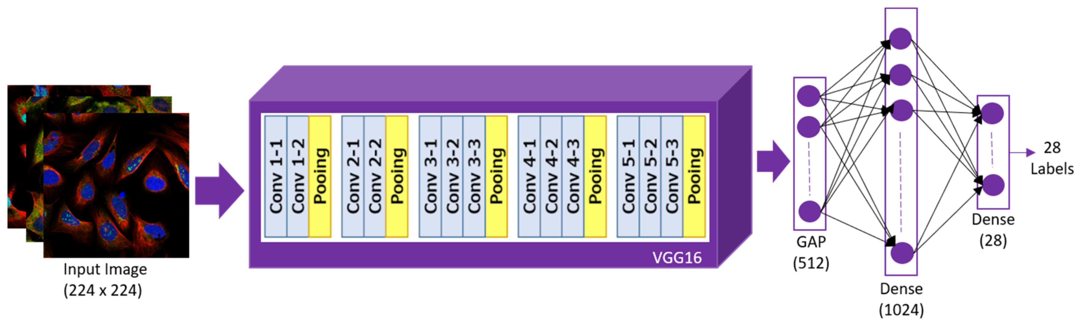
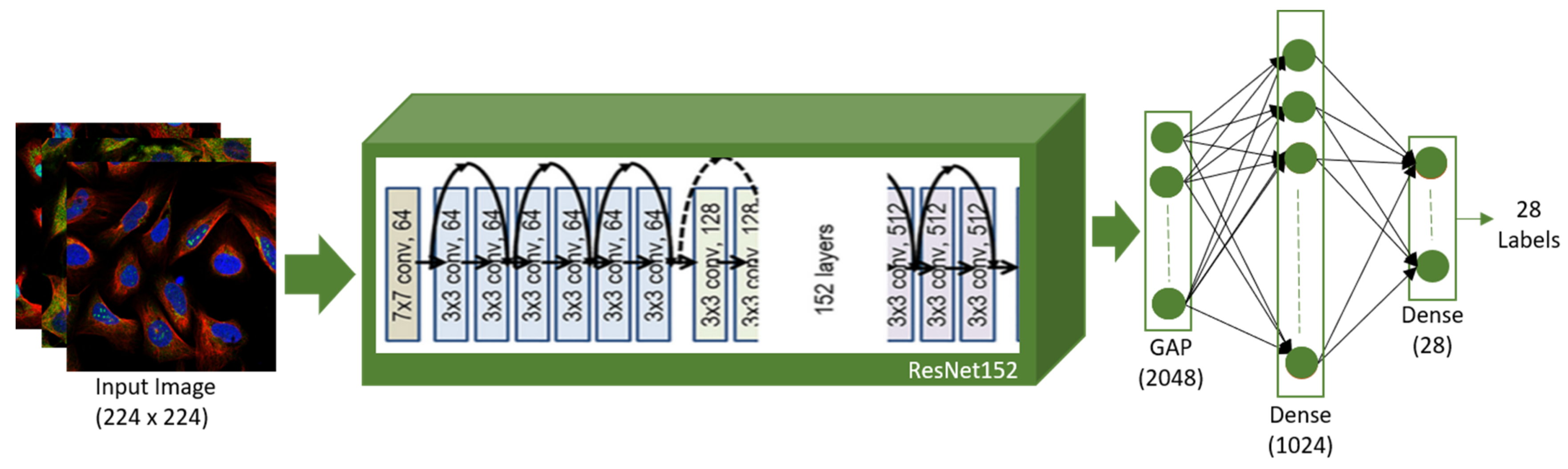
• Three transfer learning models namely VGG16, ResNet152, and DenseNet169 have been used for protein subcellular localization prediction in 28 subcellular compartments and their evaluation of the three models has been conducted on the basis of precision, recall, and F1-score.
• Further improvement in results has been achieved by proposing a stacked ensemble model using the predictions obtained from three transfer learning models, and it has also been evaluated on the basis of precision, recall, and F1 score.
• Comparison in the performance of proposed stacked ensemble model has been made with the three transfer learning models.

The rest of the article is organized as follows: The contributions made for protein subcellular localization prediction are highlighted in Section 2. The materials and methods followed by dataset utilization and the proposed model’s architecture have been explained in Section 3. Section 4 presents the results and discussion which contains the detailed experimental setup along with the analysis of the results. The concluding remarks, the shortcomings, as well as future opportunities are outlined in Section 5.

2. Related Work

Methods that integrate fluorescence microscopy with deep learning and machine learning approaches have been developed during the last decade to analyze protein localization in cultured cells systematically [28]. These approaches involve the extraction of subcellular location features (SLFs) from microscopic images [29]. SLFs comprise morphological features, wavelet features, Haralick features, and Zernike moment features, all of which are numerical characteristics that define subcellular distributions quantitatively. After being extracted from images, SLFs can be used for developing classifiers to discriminate different protein patterns.

Tahir et al. [30] extracted subcellular location features like Haralick textures, linear binary patterns, and histograms of oriented gradients from microscopic images and applied random forest and rotation forest classifiers for classification. They also balanced the data using SMOTE technique and achieved an F1-score of 0.53 on the images of the Chinese Hamster Ovary dataset. Tahir et al. [31] also extracted subcellular location features from the microscopic images obtained from HeLa and CHO dataset, and the prediction was made using the ensemble of support vector machine (SVM) classifier and achieved F1-score of 0.31 on HeLa and 0.64 on CHO dataset. Though machine learning techniques for the localization of protein are successful, they involve time-consuming manual feature extraction from images. By allowing the model to learn feature representations independently, in deep learning feature extraction does not need to be conducted separately.

Deep learning models have been used for numerous applications such as facial recognition [32], image segmentation and classification [33], and many others [34]. Techniques based on CNN for predicting protein patterns have also recently been deployed with effectiveness. A neural network is used by Boland et al. [35] for detecting protein in 2D and 3D microscopic images. A model based on SVM and an ensemble model for protein localization has been developed by Huang et al. [36]. Justin et al. [37] introduced two novel classifiers based on random forest and SVM that dramatically increased protein subcellular location detection accuracy. Coelho et al. [38] produced two new protein datasets using microscopic images to automate the protein subcellular localization prediction using CD tagging. They combined K-means and SVM to improve the classification. With 55% accuracy, Lu et al. devised a supervised learning technique to learn patterns in single cells using microscopic imagery [39]. Liimatainen et al. [40] employed microscopic images to identify the protein’s location using CNN and FCN. FCN outperformed CNN, with an F1-score of 0.696. Li et al. [41] proposed a model achieving an F1-score of 0.706 that was created with an Inception V3 pretrained model. Using two different algorithms, Shwetha et al. [42] classified images from the HPA database. Two techniques were used. In the first technique, the random forests classifier was utilized for classification. The second method extracted features and classified them into 15 different classes using two different architectures, namely Xception and ResNet 50. The F1-score of the Hybrid Xception model was 0.69, compared to 0.61 for the traditional approach. Sullivan et al. [43] used a mixture of two techniques to classify fluorescent microscopic images from the Human Protein Atlas dataset. An online video game competition was hosted by the first for the classification of images, from which 33 million annotations of protein location were obtained. Then, using the outcomes of the online video game competition, an automated algorithm named Loc-CAT was created to classify protein localization into 29 subcellular compartments. The two strategies were then combined using transfer learning to develop a model for categorizing protein patterns with an F1-score of 0.72. Kraus et al. [44] created DeepLoc i.e a CNN with 11 layers to assess the localization of the proteins in yeast, achieving 72.3%. Chang et al. [45] applied ResNet on microscopic images from the HPA dataset and achieved an F1-score of 0.3459.

In the literature, some authors have also developed ensemble learning-based models using classifiers based on machine learning for protein location prediction and achieved good results. Ensemble learning concatenates the predictions of more than one model to achieve better results. The model presented by Zhang et al. [46] is made up of two cascading ensembles. The initial group of classifiers was a collection of binary SVMs that could be trained to perform broad classification tasks. The second set used 3 classifiers including multiple-layer perceptron, multi-class SVM, and the random forest classifier. Features were extracted manually and an accuracy of 96% was achieved using 2D HeLa cell images. Another ensemble learning-based model was proposed by Muhammad Tahir et al. [47] consisting of an ensemble of SVMs. They achieved an accuracy of approx. 99% to classify protein location in 10 subcellular compartments on images procured from HeLa and LOCATE datasets.

As a result of better results obtained in the literature using an ensemble of machine learning classifiers, we implemented the ensemble learning technique using neural networks on the HPA dataset. The novelty of our work is that we have used an ensemble learning technique using neural networks, which have not been deployed for protein localization to date. The main advantage of using deep learning models like transfer learning models is that feature extraction need not be conducted manually, and also these models have been pretrained on a huge ImageNet dataset, which makes feature extraction easier and also helps to achieve good results.

3. Materials and Method

The dataset utilized in this study is described in detail in this section. In addition, the preprocessing of the images before feeding them to the model has been explained. This section also covers the methods utilized in this study, including a detailed description of the proposed model’s architecture and parameters employed in its training.

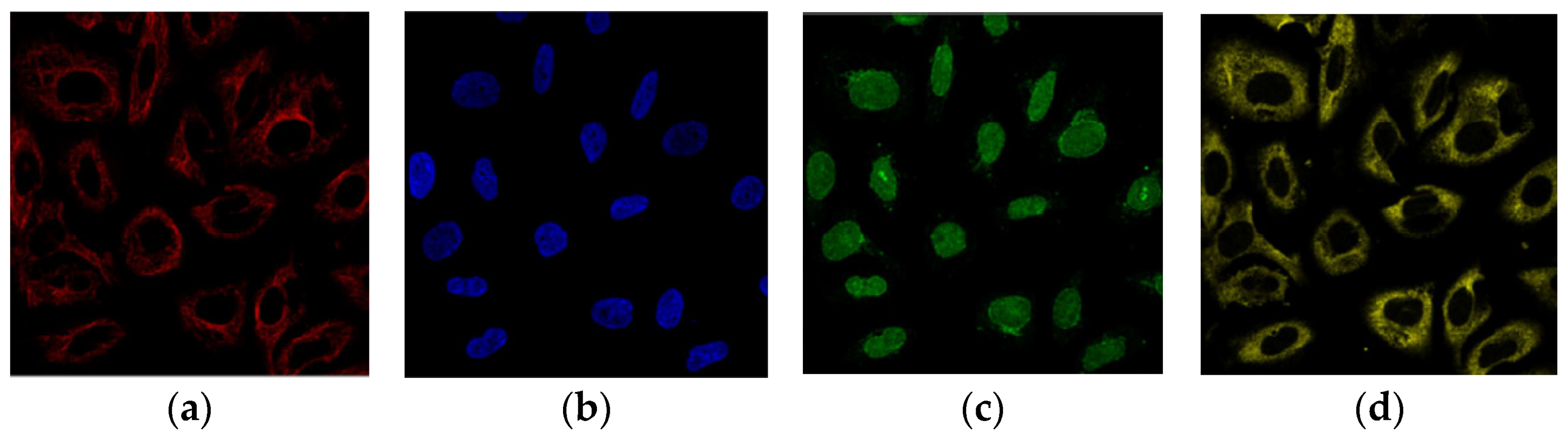
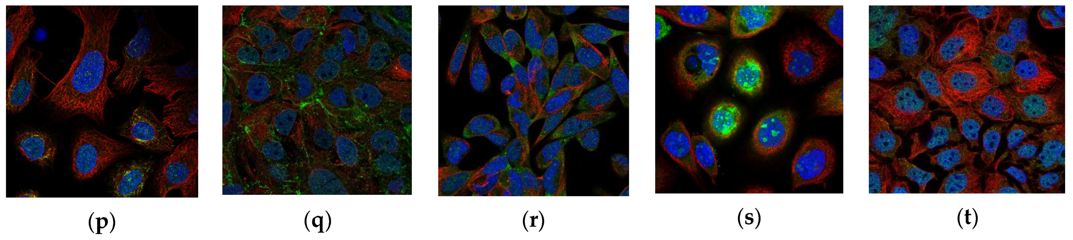
3.1. Dataset Description

The dataset is obtained from the “Human Protein Atlas Image Classification” crowdsourcing competition on Kaggle [48]. Confocal microscopy, a highly homogeneous imaging technique, was used to create this dataset. In the database, there are 31,072 samples. As shown in Figure 1, every sample consists of four images. These 4 images are labeled with a distinct fluorescent protein marked with red, blue, green, and yellow colors. We used three of the four images offered for one sample in this analysis (red, blue, and green).

Proteins have been distributed into 28 subcellular compartments in this dataset. Therefore, there are 28 different classes in this dataset into which classification must be done. It’s also possible for a single image to belong to many classes. As a result, this is a multi-label classification challenge.

Table 1. Sample distribution of each label in training and test data.

Label No.	Label Name	Total	Train	Test
0	Nucleoplasm	12,885	10,306	2579
1	Nuclear Membrane	1254	999	255
2	Nucleoli	3621	2880	741
3	Nucleoli Fibrillar Center	1561	1282	279
4	Nuclear Speckles	1858	1499	359
5	Nuclear Bodies	2513	1994	519
6	Endoplasmic Reticulum	1008	811	197
7	Golgi Apparatus	2822	2251	571
8	Peroxisomes	53	42	11
9	Endosomes	45	36	9
10	Lysosomes	28	22	6
11	Intermediate Filaments	1093	888	205
12	Actin Filaments	688	560	128
13	Focal Adhesion Sites	537	430	107
14	Microtubules	1066	839	227
15	Microtubule End	21	17	4
16	Cytokinetic Bridge	530	419	111
17	Mitotic Spindle	210	165	45
18	Microtubule Organizing Centre	902	701	201
19	Centrosome	1482	1178	304
20	Lipid Droplets	172	143	29
21	Plasma Membrane	3777	3010	767
22	Cell Junctions	802	648	154
23	Mitochondria	2965	2358	607
24	Aggresome	322	255	67
25	Cytosol	8228	6560	1668
26	Cytoplasmic Bodies	328	260	68
27	Rods and Rings	11	9	2

provides the names of the 28 different classes. Since four separate filters are provided for one image sample, data preparation was completed first by combining the three images belonging to the red, green, and blue filters. After combining the three channels, sample images obtained from the database are presented in Figure 2. The single or multiple labels to which they belong are mentioned in the image description.

The dataset was split into two parts: training and testing data. Eighty percent of image samples belonged to training data and twenty percent belonged to testing data. Data splitting was completed with an iterative stratification split module from the scikit multi-learn library. Iterative stratification is useful in multi-label classification problems as it allows the balanced distribution of classes between train and test data [49]. The number of images belonging to each class and their distribution in test and training data is mentioned in Table 1. Table 1 shows that the dataset is highly imbalanced since the majority class (cytoplasm) belongs to as large as 12,885 image samples, while the minority class (rods and rings) belongs to only 11 image samples. This severe skewness in the dataset poses a significant challenge for accurate multi-label classification.

3.2. Data Pre-Processing

Pre-processing was completed on the microscopic images before they were fed into the model for training. To begin, all images were scaled to 224 × 224 pixels using the open-cv library to be used as input tensors for pretrained CNN networks with predefined image shapes. The capacity of the model to predict has been observed to be unaffected by image scaling. If, on the other hand, the default image size is used, the number of parameters will substantially increase, leaving the model computationally costly. Finally, data normalization was completed by scaling the pixel values in the range of 0 to 1. Normalization was completed by dividing every pixel by 255. The step of data normalization ensures that every pixel has a uniform data distribution. After normalization, it was observed that the model was more quickly and effectively trained.

3.3. Architecture of Fine-Tuned Transfer Learning Models

For the challenge of protein subcellular localization prediction, researchers have used a variety of models in the literature. However, the majority of the models employ machine learning techniques, which include manual feature extraction followed by a machine learning classifier. Yet, in real time, manual feature extraction is tedious since it needs a human expert. In this research, we have used deep learning-based models which do not require manual feature extraction. This makes our model practicable in real time, as we have trained our model using raw images with minimal pre-processing. When deep learning models are trained on large datasets, they have the potential to yield exceptional results.

Due to data scarcity in some applications, such as medical imaging, expanding training samples is not always practical. Transfer learning may be beneficial in such areas. A model trained on a bigger database, such as ImageNet, can be utilized in transfer learning for tasks that are equivalent to domains with small datasets. There are many applications where transfer learning has been applied successfully, for example, automation, medical imaging, and manufacturing [50].

In this study, three pretrained transfer learning models, namely, VGG16 [51], DenseNet169 [52], and ResNet152 [53,54], have been used for HPA image classification. Instead of starting from scratch to build a CNN model, the proposed approach relies on pretrained models with fine-tuned top layers [55]. The initial layers of any CNN-based model extract edges, lines, blobs, and other low-level features. To solve any image classification task, the effective extraction of such low-level features is required [56]. Because the weights of pretrained models have been significantly refined on a bigger dataset, the suggested method focuses solely on fine-tuning the top layers by freezing initial layers to maximize the high-level features [57]. The modified architectures of the pretrained transfer learning models chosen for this study are depicted in Figure 3, Figure 4 and Figure 5. As shown in the figures, the head of the model was replaced with a set of new layers, including a pooling layer and a fully connected layer with 1024 nodes. Lastly, another fully connected layer with a sigmoid activation function is used as a final layer that predicts 0 and 1 for the 28 labels [58]. Following the fine-tuning of the top layers, the other layers were also trained at a meager learning rate to ensure that their pretrained weights did not change significantly. Then, to achieve outstanding results, an ensemble of the models indicated above was developed. The following sections provide background information on each transfer learning model [59,60].

3.4. Architecture of VGG16

Simonyan et al. [51] proposed this architecture. In the 2014 ILSVRC competition, VGG16 was one of the top performers. The small kernel size of this network is its key distinguishing feature. It employs a 3 × 3 kernel that is repeated in the layers 256 and 512 times. This aids the model in capturing localized properties unique to a specific class, hence enhancing classification accuracy. Using a smaller kernel size in VGG16 architecture imposes several disadvantages. Because of the small size of convolutions applied, it leads to an increase in the number of training parameters. Pooling layers are also used in VGG to reduce the model’s complexity by eliminating unnecessary features [61,62,63]. The architecture of the modified VGG16 is presented in Figure 3.

3.4.1. Architecture of ResNet152

The vanishing/exploding gradient problem is solved using ResNet, a residual learning framework [64]. Skip connections are employed in this network. The skip connection links straight to the output after skipping a few stages of training. The benefit of including this type of skip connection is that regularization will skip any layer that degrades the architecture’s performance [65] As a result, an intense neural network can be trained without the issues caused by vanishing/exploding gradients. ResNet152 [52] is a 152-layer CNN, and its modified architecture is displayed in Figure 4.

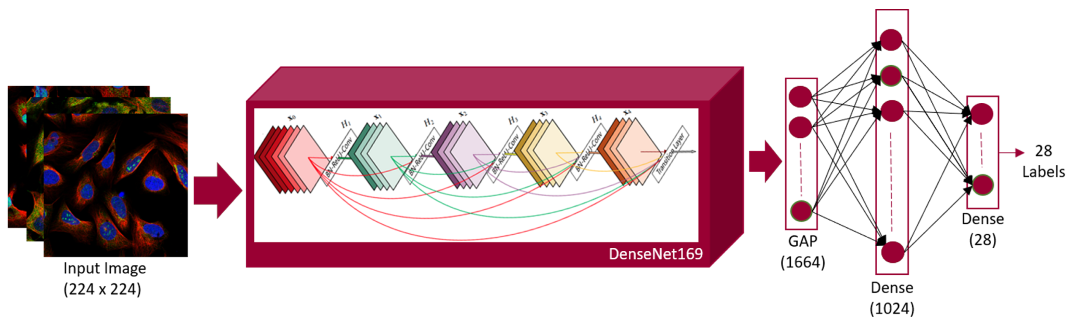
3.4.2. Architecture of DenseNet169

As a result of improved accuracy by the vanishing gradient, DenseNet [66] was chosen as a component model for the ensemble. Because of the long distance between the input and output layers of neural networks, information may be lost before reaching the last layer [67]. Every layer in the DenseNet model receives more data from the previous layers before passing its feature maps to all layers. The model conducts information concatenation, and each layer acquires collective knowledge from the layers before it [68]. This model is 169 layers deep, and its modified architecture is shown in Figure 5.

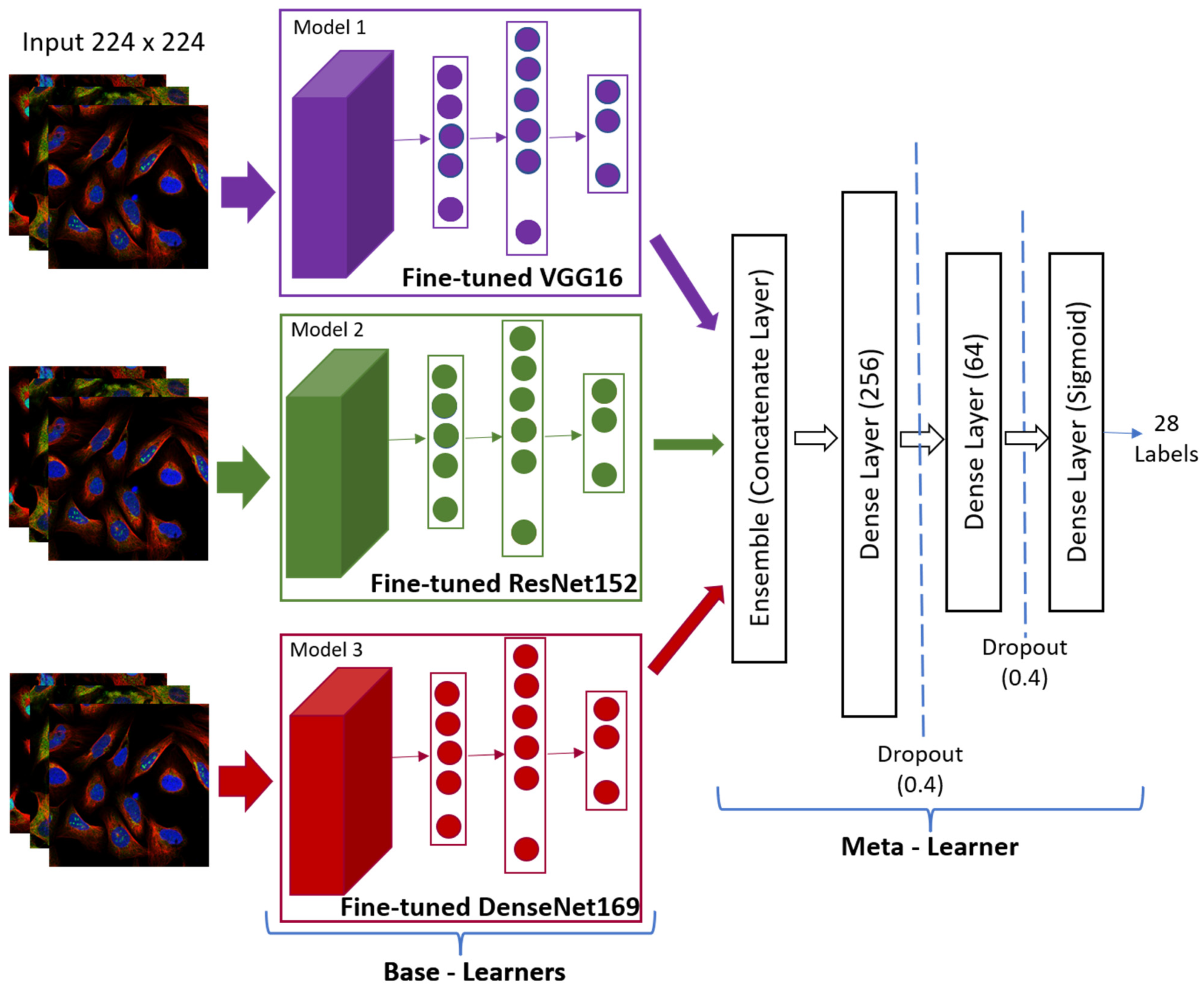
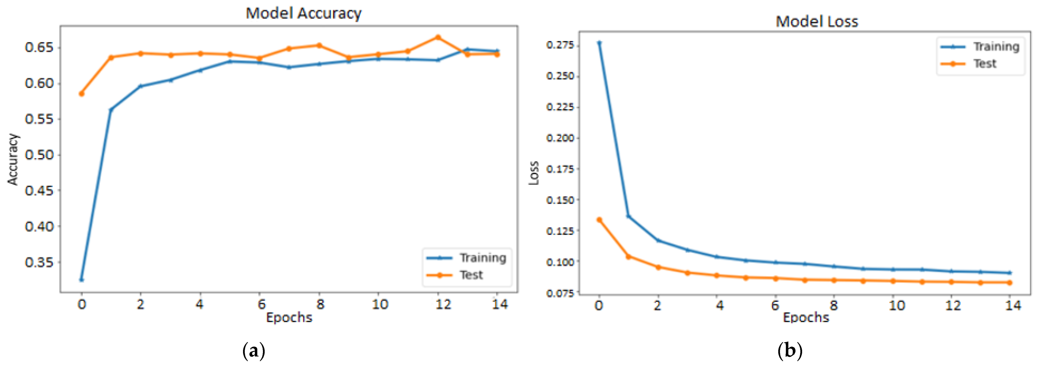
3.4.3. Architecture of the Proposed Stacked Ensemble Model

Because each convolutional neural network has a varied number of layers and network architecture, its performance on various tasks differs [69]. Furthermore, when applied to medical images, each pretrained model has its own set of strengths and limitations. We can train many models on a similar dataset, make predictions, and combine findings to attain the best performance in the ensemble learning strategy. Ensemble learning has been shown to minimize variation and enhance performance significantly [70]. Taking an average of the predictions predicted from individual models on a similar group of training and test data is the simplest technique to integrate the predictions of many trained models [71]. Averaging ensemble provides combined forecasts by evenly combining predictions from numerous trained models. Another technique is the weighted average ensemble method that provides weights to individual model predictions that are tuned using validation data [72].

The stacked ensemble approach is another prevalent method [73]. It is a refined version of an average ensemble that incorporates the post-training of the new model created by combining many sub-models. A stacked ensemble entails two or more base models or base learners and a meta-model or level 1 model [74]. Base learners are the models trained on the training dataset and their predictions are concatenated, while meta-learner learns how to concatenate the predictions obtained from base models. The training of meta-learner is completed on the predictions concatenated from base learners on the hold-out dataset or test dataset. The architecture of proposed stacked ensemble model is given in Figure 6.

3.5. Experimental Setup

Various hyper-parameters were modified during deep neural network training to achieve better outcomes as presented in

Table 2. Hyperparameter Settings.

Hyper-Parameters	Values
Mini Batch Size	32
Initial Learning Rate	0.001
Weight Decay	1.0 × 10−8
Beta	0.9, 0.999
Optimizer	Adam (Default Parameter)

. Pretrained models had all their layers frozen at the beginning of the process, and only new layers used as the head of the network were trained. The training was completed for 15 epochs with learning rate of 1 × 10⁻³. Adam was used as an optimizer with default parameters [56] as mentioned in Table 2. Thereafter, the models were fine-tuned by training all the layers for 20 epochs with average small learning rate of 1 × 10⁻⁵. After training pretrained models, predictions obtained from them were concatenated to form a feature vector fed to the meta-learner. At this time, all the pretrained models were frozen and training of meta-learner was completed for 25 epochs with a learning rate of 1 × 10⁻³. Early stopping callback with patience of 4 epochs was used as a regularization method to avoid overfitting during the training of both pretrained models and meta-learner. Binary cross entropy was utilized as a loss function due to the multi-label nature of the dataset. Due to the limitations of the available GPU RAM, a batch size of 32 was chosen for simulation. All the experiments were carried out on the Kaggle platform with enabled GPU hardware as an accelerator.

3.6. Performance Metrics

For each class, the following criteria were chosen to evaluate the results of classification problems: recall and precision. Precision is the fraction of correctly predicted positive instances to overall predicted positive instances. It assesses the quality of positive predictions, whereas recall assesses the number of positive predictions. Recall is given by the percentage of positive samples that are predicted to be positive out of all positive samples. Precision, F1-score, and recall are calculated independently for all the labels in a multi-label classification problem. Since this study relies on an imbalanced dataset, each label’s sample numbers must be considered while computing the performance measures. Therefore, weighted recall, F1-score, and precision were also calculated and are shown in

Table 3. Performance of the fine-tuned transfer learning models.

Model	VGG16			ResNe152			DenseNet169
Label No.	Precision	Recall	F1-Score	Precision	Recall	F1-Score	Precision	Recall	F1-Score
0	0.80	0.86	0.83	0.78	0.85	0.81	0.77	0.83	0.80
1	0.83	0.68	0.75	0.74	0.55	0.63	0.65	0.52	0.58
2	0.71	0.66	0.68	0.69	0.65	0.67	0.64	0.64	0.64
3	0.49	0.51	0.50	0.48	0.45	0.47	0.44	0.37	0.40
4	0.65	0.70	0.67	0.76	0.61	0.68	0.69	0.63	0.66
5	0.65	0.42	0.51	0.35	0.44	0.39	0.35	0.41	0.38
6	0.46	0.53	0.49	0.47	0.49	0.48	0.43	0.45	0.44
7	0.75	0.64	0.69	0.63	0.54	0.58	0.61	0.48	0.54
8	0.11	0.45	0.17	0.50	0.27	0.35	0.07	0.09	0.08
9	0.23	0.67	0.34	1.00	0.22	0.36	0.33	0.11	0.17
10	0.15	0.50	0.23	0.67	0.33	0.44	0.25	0.17	0.20
11	0.77	0.54	0.64	0.66	0.55	0.60	0.70	0.47	0.57
12	0.67	0.46	0.55	0.52	0.48	0.50	0.48	0.48	0.48
13	0.55	0.54	0.55	0.68	0.41	0.51	0.71	0.43	0.53
14	0.84	0.81	0.82	0.88	0.80	0.84	0.89	0.78	0.83
15	1.00	0.25	0.40	0.00	0.00	0.00	0.00	0.00	0.00
16	0.47	0.15	0.23	0.20	0.26	0.23	0.16	0.18	0.17
17	0.30	0.18	0.22	0.13	0.29	0.18	0.41	0.24	0.31
18	0.38	0.40	0.39	0.35	0.44	0.39	0.22	0.36	0.27
19	0.37	0.50	0.43	0.30	0.32	0.31	0.21	0.34	0.26
20	0.13	0.52	0.20	0.44	0.24	0.31	0.26	0.34	0.30
21	0.64	0.64	0.64	0.63	0.63	0.63	0.62	0.65	0.63
22	0.44	0.51	0.47	0.49	0.39	0.43	0.50	0.35	0.41
23	0.75	0.69	0.72	0.71	0.68	0.69	0.70	0.63	0.66
24	0.74	0.60	0.66	0.65	0.49	0.56	0.56	0.49	0.52
25	0.63	0.76	0.69	0.63	0.72	0.68	0.63	0.73	0.67
26	0.26	0.32	0.29	0.22	0.28	0.25	0.09	0.28	0.14
27	0.00	0.00	0.00	0.00	0.00	0.00	0.00	0.00	0.00
Weighted Average	0.67	0.68	0.67	0.64	0.65	0.64	0.62	0.63	0.62

and

Table 4. Precision, Recall, and F1-score of the proposed Ensemble Model.

Label No.	Label Name	Precision	Recall	F1-Score
0	Nucleoplasm	0.79	0.90	0.84
1	Nuclear Membrane	0.84	0.69	0.76
2	Nucleoli	0.72	0.75	0.73
3	Nucleoli Fibrillar Center	0.60	0.47	0.53
4	Nuclear Speckles	0.81	0.67	0.73
5	Nuclear Bodies	0.56	0.52	0.54
6	Endoplasmic Reticulum	0.60	0.51	0.55
7	Golgi Apparatus	0.76	0.67	0.71
8	Peroxisomes	0.29	0.18	0.22
9	Endosomes	0.70	0.56	0.63
10	Lysosomes	1.00	0.50	0.67
11	Intermediate Filaments	0.81	0.59	0.68
12	Actin Filaments	0.67	0.55	0.60
13	Focal Adhesion Sites	0.73	0.52	0.61
14	Microtubules	0.92	0.83	0.87
15	Microtubule End	0.50	0.25	0.33
16	Cytokinetic Bridge	0.41	0.19	0.26
17	Mitotic Spindle	0.34	0.24	0.29
18	Microtubule Organizing Center	0.45	0.44	0.45
19	Centrosome	0.45	0.48	0.46
20	Lipid Droplets	0.41	0.24	0.30
21	Plasma Membrane	0.74	0.64	0.68
22	Cell Junctions	0.58	0.45	0.51
23	Mitochondria	0.81	0.69	0.74
24	Aggresome	0.81	0.64	0.55
25	Cytosol	0.75	0.80	0.72
26	Cytoplasmic Bodies	0.67	0.79	0.72
27	Rods and Rings	0.00	0.00	0.00
Weighted Average		0.72	0.70	0.71

, considering the number of samples belonging to each label.

4. Results and Discussions

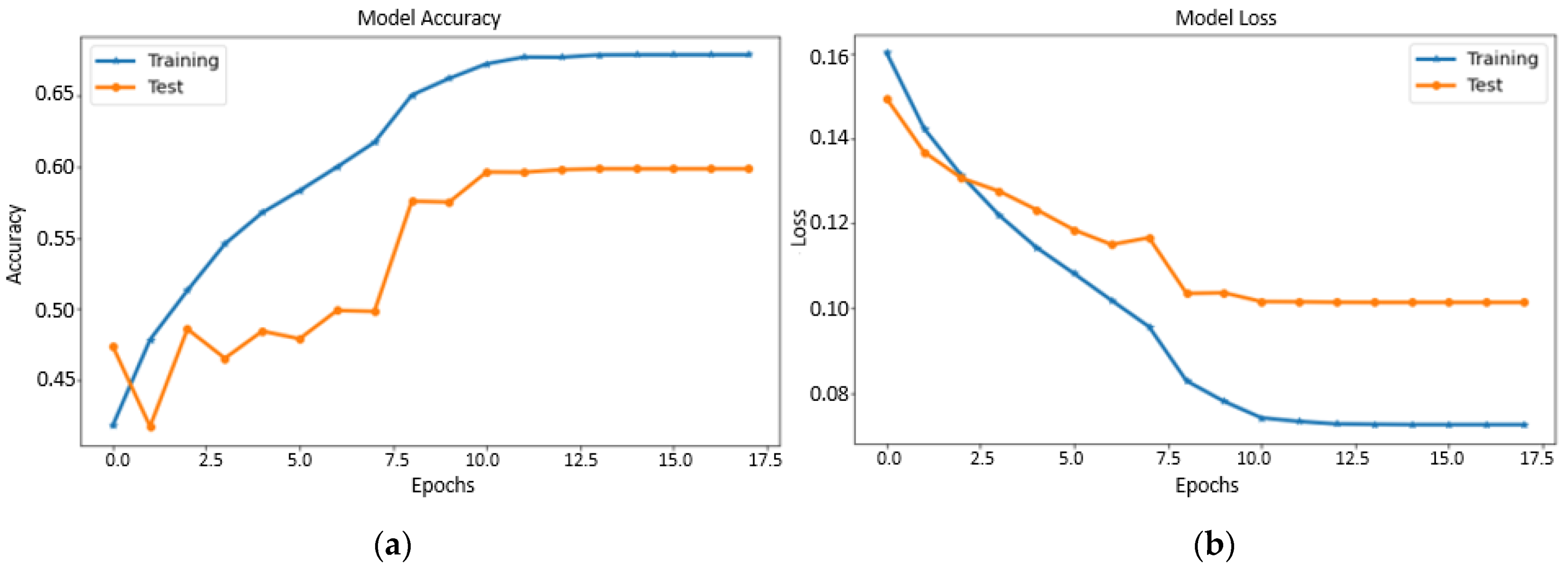
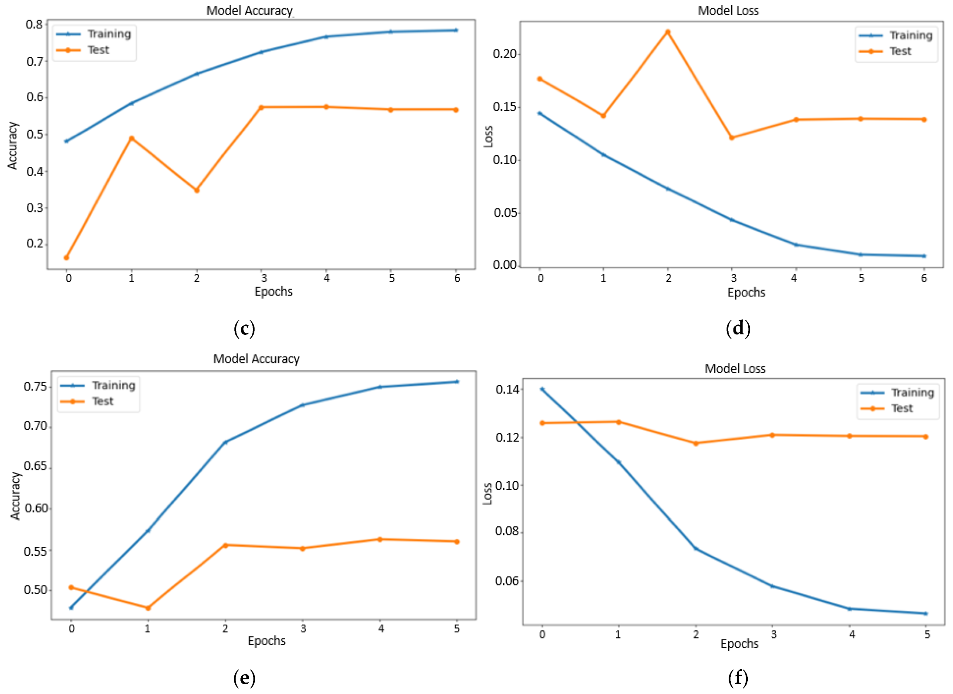
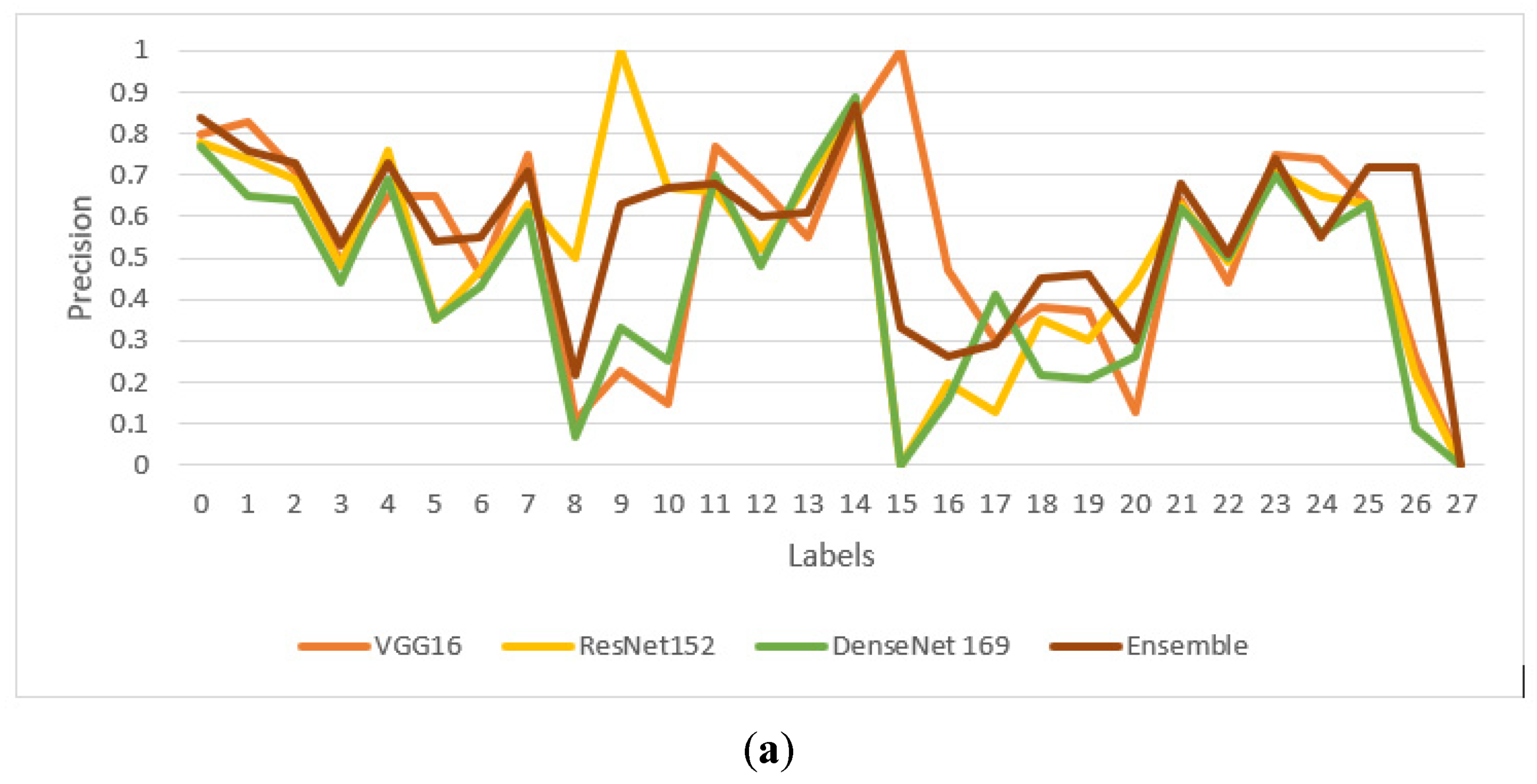
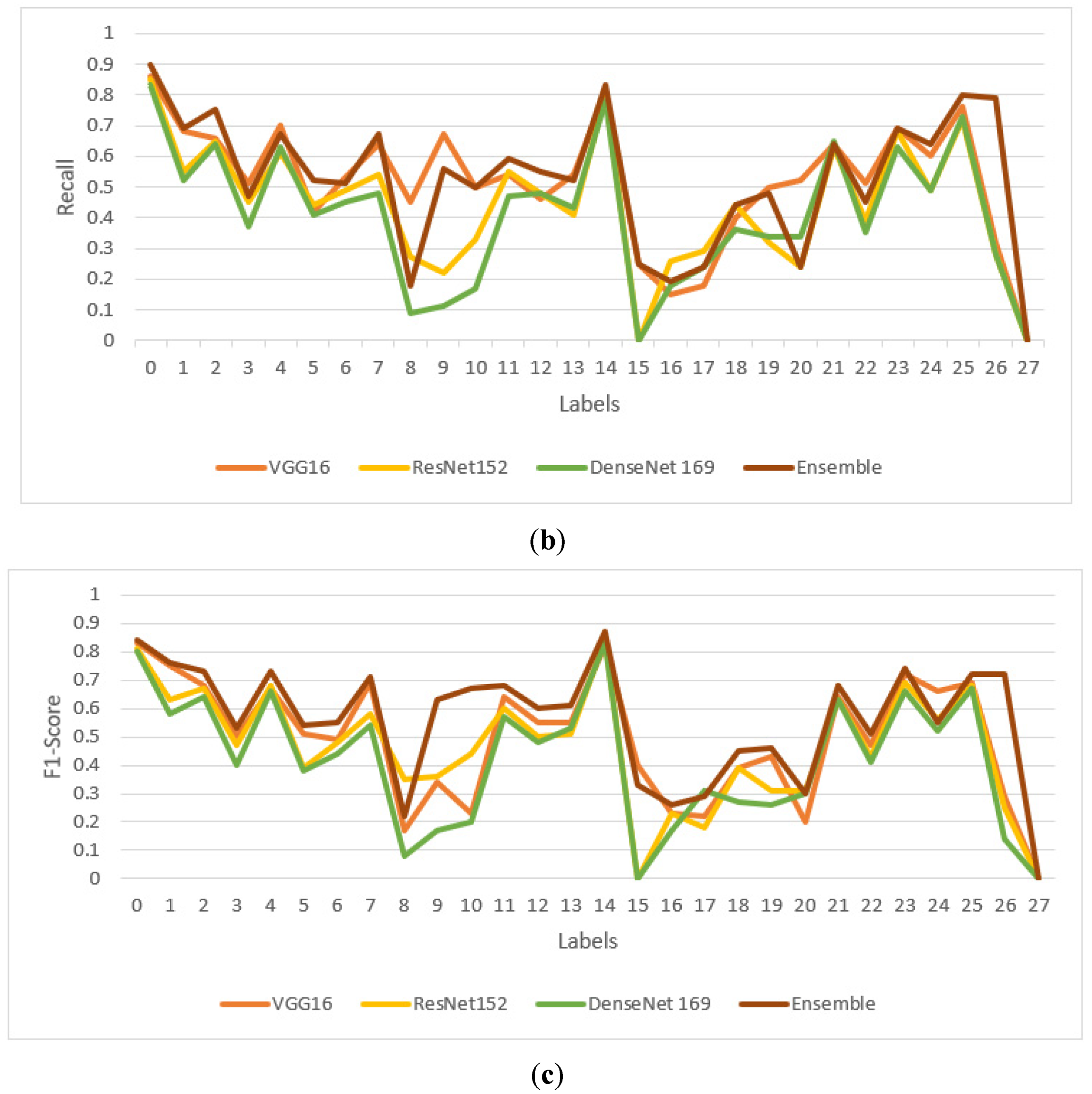
4.1. Performance of Fine-Tuned Pretrained Transfer Learning Models

In this research, three pretrained models, namely VGG16, ResNet152, and DenseNet169, have been used as the base learners. These models were trained, evaluated, and saved independently to be used for the staked ensemble approach. Loss and accuracy plots of the pretrained models are displayed in Figure 7. Figure 7a shows that training and test accuracy of 68% and 58%, respectively, were achieved using the VGG16 model; Figure 7c shows that training and test accuracy of 80% and 50%, respectively, were achieved using ResNet152; and Figure 7e shows that training and testing accuracy of 75% and 55%, respectively, were attained using DenseNet 169. Although all the models were trained for 30 epochs, their plots show different epochs because the training was stopped using an early stopping call back to avoid overfitting the models. Similarly, loss plots for the three models are given in Figure 7b,d,f.

As shown in Table 3, the three models were evaluated on the test dataset based on recall, precision and F1-score. The three performance criteria were calculated for all the labels. Table 3 shows that VGG16 performed best by attaining 0.67 precision, 0.68 recall, and 0.67 F1 score. However, since every model has its own advantages and limitations, as they differ in their depth and architecture, instead of selecting the best model, an ensemble approach has been proposed. As can be seen from Table 3, label 0 (nucleoplasm) was best predicted by VGG16 than the other two models. Similarly, label 10 (lysosomes) and label 14 (microtubules) were predicted best by ResNet152, and label 17 (microtubule ends) was best predicted by DenseNet169. Hence, to achieve better results, the predictions obtained from the three base learners were combined and fed to another meta-learner, creating a stacked ensemble.

4.2. Performance of the Proposed Stacked Ensemble Model

The ensemble model proposed in this research has been built by stacking the three base learners whose predictions are combined and fed as input to the meta-learner. The meta-learner we have employed is a fully connected network, which allows the stacked model to be flexible while also reducing generalization error. Because the neural network incorporates the predictions from each of the underlying models, the overall performance of the model is enhanced. To increase classification accuracy, the neural network has been tuned to ignore the incorrect predictions produced by the base models. Because various CNN models make errors in the classification of different samples, combining them helps to improve test set outcomes.

The accuracy and loss plots of the stacked ensemble model are shown in Figure 8. As can be seen from Figure 8a, training and testing accuracy of approximately 65% is achieved, and Figure 8b shows validation loss reaches 0.08 approximately. Table 4 displays recall, precision, and the F1-score achieved for every label as well as their combined values for the model. It can be inferred using Table 4 that almost every label has a better F1 score than the individual separate models. Hence, the classification results improved when the predictions were made on the test dataset using a stacked ensemble to those made on the individual transfer learning models.

4.3. Performance Comparison of Proposed Model with Transfer Learning Models

Figure 9 compares the performance of the three transfer learning models and the proposed ensemble models. Figure 9a compares precision across all the labels for the four models. However, some labels might show better precision results for transfer learning models than the ensemble model. Yet even then, Table 4 shows that the ensemble model achieved the highest average precision of 0.71 among all the four models. Similarly, Figure 9b,c compare the recall and F1-score achieved across all labels for all four models. Again, the proposed ensemble model achieved the highest average value of F1-score and recall with 0.71 and 0.70, respectively.

Additionally, the cost efficiency of a model can be measured based on the time taken to train a model. In this research, all the models have been run on a publicly available Kaggle platform with a GPU accelerator. The time taken to train each model has been compared in

Table 5. Comparison of Time Taken to Train Different Models.

Model Name	Time Taken to Train the Model
Fine-tuned VGG16	10,839.0 s
Fine-tuned ResNet152	11,099.3 s
Fine-tuned DenseNet169	16,928.5 s
Proposed Ensemble Model	5564.8 s

. From Table 5, it can be inferred that less time was taken to achieve results from the proposed ensemble model as compared to individual transfer learning models. So, it can be concluded that the ensemble learning-based technique makes our model cost-efficient.

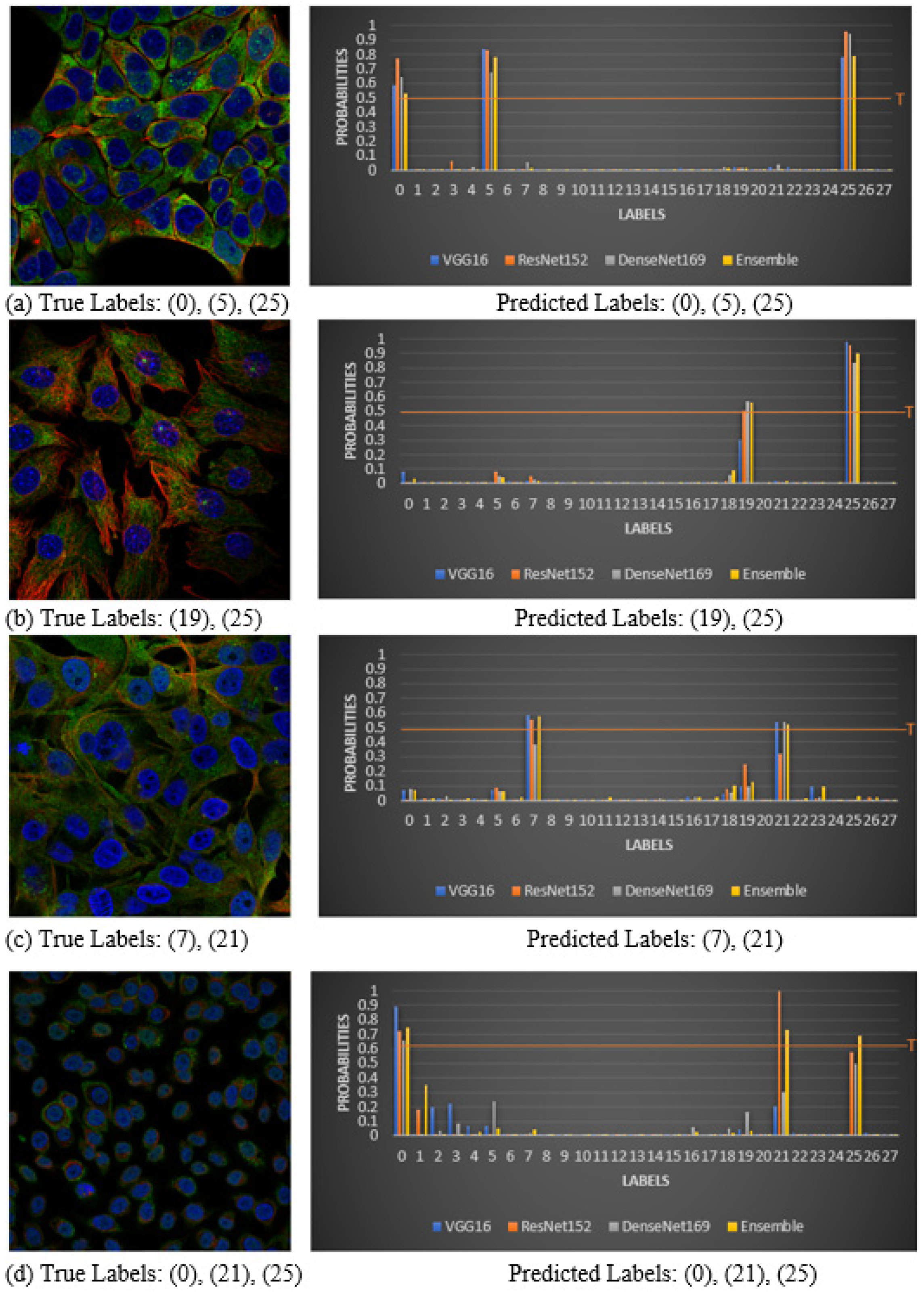
4.4. Visualization of Correct Classifications

Figure 10 depicts some examples of correct classification performed by transfer learning models and the ensemble model. To obtain predictions of 0 and 1 for each label from the sigmoid layer of the pretrained and ensemble models, the threshold level was set to 0.5. For example, in Figure 10b, the true labels for the sample image are 19 and 25. The ensemble model predicted the same labels, as evidenced by the corresponding graph. As a result, this is an example of correct classification. However, it can be seen that the probability obtained from VGG16 for label 19 is less than 0.5, whereas the probability obtained from the other two pretrained models is greater than 0.5. Even so, the ensemble model correctly predicted label 19. This demonstrates that the ensemble model combines predictions from multiple models to produce the best result. Figure 10 also shows that labels 0 and 25 have been predicted more confidently by all the models, because these are the majority classes.

4.5. Visualization of Incorrect Classifications

Figure 11 shows some examples of incorrect classification performed by transfer learning models and the ensemble model. For example, in Figure 11b, the true labels for the sample image are 0 and 25. Yet the ensemble model predicted one extra label, that is 23, as evidenced by the corresponding graph. So, this is an example of incorrect classification. It can also be observed from Figure 11 that label 23 has been predicted for almost all the images, even though it is not shown by actual labels. Moreover, Figure 11c shows there were three labels in the image, but the model could only predict one label correctly.

4.6. Comparison with State-of-Art

A comparison of the proposed model’s performance with the state-of-art methods is shown in

Table 6. Comparison of the proposed model with the state-of-art techniques.

Reference No.	Dataset Used	Technique	F1-Score
[30]	Chinese Hamster Ovary (CHO) Dataset	Random Forest and Rotation Forest	0.53
[31]	CHO Dataset	Ensemble of SVM classifier	0.64
[40]	HPA Dataset	FCN CNN	0.696 0.676
[41]	HPA Dataset	Inception V3	0.706
[42]	HPA Dataset	Hybrid Xception	0.69
[45]	HPA Dataset	ResNet	0.3459
Proposed Model	HPA Dataset	Stacked Ensemble of Transfer Learning models	0.71

. The performance criterion selected for the comparison is the F1-score, as it gives us the harmonic mean of recall and precision. Table 6 shows that the proposed model’s performance is better than the state-of-the-art deep learning models, as it improved the F1-score by 0.1.

5. Conclusions and Future Scope

In this research, three pretrained models, namely VGG16, ResNet152, and DenseNet 169, were used to predict protein subcellular location in microscopic images procured from HPA Database. The three said models achieved an F1-score of 0.67, 0.64, and 0.62, respectively. Yet, instead of selecting the best model among the three, this article proposed a stacked ensemble approach that combined the power of the three pretrained models and achieved a better F1-score of 0.71. The result shows that assembling different weak convolutional neural networks results in better predictions than single models.

The main limitation of this research work was the huge class imbalance observed in the dataset. In addition, there were some labels for which very few images were provided, which were insufficient to train the model. More samples for the minority classes will be collected in future work to achieve better results. Data balancing techniques can also be applied to balance the data, and samples for minority classes can also be increased by using data augmentation techniques. Furthermore, instead of using pretrained models, CNN from scratch can also be built for the multi-label HPA classification.

References

1. Butler, G.S.; Overall, C.M. Proteomic identification of multitasking proteins in unexpected locations complicates drug targeting. Nat. Rev. Drug Discov. 2009, 8, 935–948. [Google Scholar] [CrossRef]
2. Hung, M.C.; Link, W. Protein localization in disease and therapy. J. Cell Sci. 2011, 124, 3381–3392. [Google Scholar] [CrossRef] [PubMed] [Green Version]
3. Pepperkok, R.; Ellenberg, J. High-throughput fluorescence microscopy for systems biology. Nat. Rev. Mol. Cell Biol. 2006, 7, 690–696. [Google Scholar] [CrossRef] [PubMed]
4. Uhlen, M.; Oksvold, P.; Fagerberg, L.; Lundberg, E.; Jonasson, K.; Forsberg, M.; Zwahlen, M.; Kampf, C.; Wester, K.; Hober, S.; et al. Towards a knowledge-based human protein atlas. Nat. Biotechnol. 2010, 28, 1248–1250. [Google Scholar] [CrossRef]
5. Xu, Y.Y.; Yao, L.; Shen, H.B. Bioimage-based protein subcellular location prediction: A comprehensive review. Front. Comput. Sci. 2018, 12, 26–39. [Google Scholar] [CrossRef]
6. Jha, K.; Doshi, A.; Patel, P.; Shah, M. A comprehensive review on automation in agriculture using artificial intelligence. Artif. Intell. Agric. 2019, 2, 1–12. [Google Scholar] [CrossRef]
7. Limone, P.; Toto, G.A.; Guarini, P.; di Furia, M. Online Quantitative Research Methodology: Reflections on Good Practices and Future Perspectives. In Science and Information Conference; Springer: Cham, Switzerland, 2022; pp. 656–669. [Google Scholar]
8. Vincent, D.R.; Deepa, N.; Elavarasan, D.; Srinivasan, K.; Chauhdary, S.H.; Iwendi, C. Sensors driven AI-based agriculture recommendation model for assessing land suitability. Sensors 2019, 19, 3667. [Google Scholar] [CrossRef] [PubMed] [Green Version]
9. Mirbabaie, M.; Stieglitz, S.; Frick, N.R. Artificial intelligence in disease diagnostics: A critical review and classification on the current state of research guiding future direction. Health Technol. 2021, 11, 693–731. [Google Scholar] [CrossRef]
10. Chen, L.; Chen, P.; Lin, Z. Artificial intelligence in education: A review. IEEE Access 2020, 8, 75264–75278. [Google Scholar] [CrossRef]
11. Ma, Y.; Wang, Z.; Yang, H.; Yang, L. Artificial intelligence applications in the development of autonomous vehicles: A survey. IEEE/CAA J. Autom. Sin. 2020, 7, 315–329. [Google Scholar] [CrossRef]
12. Poushneh, A. Humanizing voice assistant: The impact of voice assistant personality on consumers’ attitudes and behaviors. J. Retail. Consum. Serv. 2021, 58, 102283. [Google Scholar] [CrossRef]
13. Bogatinovski, J.; Todorovski, L.; Džeroski, S.; Kocev, D. Comprehensive comparative study of multi-label classification methods. Expert Syst. Appl. 2022, 203, 117215. [Google Scholar] [CrossRef]
14. Cheng, X.; Lin, H.; Wu, X.; Shen, D.; Yang, F.; Liu, H.; Shi, N. Mltr: Multi-label classification with transformer. In Proceedings of the 2022 IEEE International Conference on Multimedia and Expo (ICME), Taipei, Taiwan, 18–22 July 2022; IEEE: Piscataway, NJ, USA, 2022; pp. 1–6. [Google Scholar]
15. Alhammad, M.; Avdelidis, N.P.; Ibarra Castanedo, C.; Maldague, X.; Zolotas, A.; Torbali, E.; Genest, M. Multi-label classification algorithms for composite materials under infrared thermography testing. Quant. InfraRed Thermogr. J. 2022, 1–27. [Google Scholar] [CrossRef]
16. Madjarov, G.; Kocev, D.; Gjorgjevikj, D.; Džeroski, S. An extensive experimental comparison of methods for multi-label learning. Pattern Recognit. 2012, 45, 3084–3104. [Google Scholar] [CrossRef]
17. Wu, G.; Zheng, R.; Tian, Y.; Liu, D. Joint ranking SVM and binary relevance with robust low-rank learning for multi-label classification. Neural Netw. 2020, 122, 24–39. [Google Scholar] [CrossRef] [Green Version]
18. Levatić, J.; Ceci, M.; Kocev, D.; Džeroski, S. Semi-supervised Predictive Clustering Trees for (Hierarchical) Multi-label Classification. arXiv 2022, arXiv:2207.09237. [Google Scholar]
19. Zhang, M.L.; Zhou, Z.H. ML-KNN: A lazy learning approach to multi-label learning. Pattern Recognit. 2007, 40, 2038–2048. [Google Scholar] [CrossRef] [Green Version]
20. Read, J.; Pfahringer, B.; Holmes, G.; Frank, E. Classifier chains for multi-label classification. Mach. Learn. 2011, 85, 333–359. [Google Scholar] [CrossRef] [Green Version]
21. Freitas Rocha, V.; Varejão, F.M.; Segatto, M.E.V. Ensemble of classifier chains and decision templates for multi-label classification. Knowl. Inf. Syst. 2022, 64, 643–663. [Google Scholar] [CrossRef]
22. Pengfei, G.; Dedi, L.; Lijiao, Z.; Yue, L.; Yinglong, M. A Three-phase Augmented Classifiers Chain Approach Based on Co-occurrence Analysis for Multi-Label Classification. arXiv 2022, arXiv:2204.06138. [Google Scholar]
23. Tsoumakas, G.; Katakis, I.; Vlahavas, I. Random k-labelsets for multilabel classification. IEEE Trans. Knowl. Data Eng. 2011, 23, 1079–1089. [Google Scholar] [CrossRef]
24. Luaces, O.; Díez, J.; Barranquero, J.; del Coz, J.; Bahamonde, A. Binary relevance efficacy for multilabel classification. Prog. Artif. Intell. 2012, 1, 303–313. [Google Scholar] [CrossRef]
25. Rastogi, R.; Mortaza, S. Imbalance multi-label data learning with label specific features. Neurocomputing 2022, 513, 395–408. [Google Scholar] [CrossRef]
26. Moyano, J.M.; Gibaja, E.; Cios, K.; Ventura, S. Review of ensembles of multi-label classifiers: Models, experimental study and prospects. Inf. Fusion 2018, 44, 33–45. [Google Scholar] [CrossRef]
27. Rokach, L.; Schclar, A.; Itach, E. Ensemble methods for multi-label classification. Expert Syst. Appl. 2014, 41, 7507–7523. [Google Scholar] [CrossRef] [Green Version]
28. Glory, E.; Murphy, R.F. Automated subcellular location determination and high-throughput microscopy. Dev. Cell 2007, 12, 7–16. [Google Scholar] [CrossRef] [PubMed] [Green Version]
29. Chen, X.; Velliste, M.; Murphy, R.F. Automated interpretation of subcellular patterns in fluorescence microscope images for location proteomics. Cytom. Part A 2006, 69A, 631–640. [Google Scholar] [CrossRef] [PubMed] [Green Version]
30. Tahir, M.; Khan, A.; Majid, A.; Lumini, A. Subcellular localization using fluorescence imagery: Utilizing ensemble classification with diverse feature extraction strategies and data balancing. Appl. Soft Comput. 2013, 13, 4231–4243. [Google Scholar] [CrossRef]
31. Tahir, M.; Khan, A. Protein subcellular localization of fluorescence microscopy images: Employing new statistical and Texton based image features and SVM based ensemble classification. Inf. Sci. 2016, 345, 65–80. [Google Scholar] [CrossRef]
32. Gadekallu, T.R.; Iwendi, C.; Wei, C.; Xin, Q. Identification of malnutrition and prediction of BMI from facial images using real-time image processing and machine learning. IET Image Process. 2021, 16, 647–658. [Google Scholar]
33. Gadamsetty, S.; Ch, R.; Ch, A.; Iwendi, C.; Gadekallu, T.R. Hash-based deep learning approach for remote sensing satellite imagery detection. Water 2022, 14, 707. [Google Scholar] [CrossRef]
34. Iwendi, C.; Moqurrab, S.; Anjum, A.; Khan, S.; Mohan, S.; Srivastava, G. N-sanitization: A semantic privacy-preserving framework for unstructured medical datasets. Comput. Commun. 2020, 161, 160–171. [Google Scholar] [CrossRef]
35. Boland, M.V.; Murphy, R.F. A neural network classifier capable of recognizing the patterns of all major subcellular structures in fluorescence microscope images of HeLa cells. Bioinformatics 2001, 17, 1213–1223. [Google Scholar] [CrossRef] [PubMed]
36. Huang, K.; Murphy, R.F. Boosting accuracy of automated classification of fluorescence microscope images for location proteomics. BMC Bioinform. 2004, 5, 78. [Google Scholar] [CrossRef] [PubMed] [Green Version]
37. Newberg, J.Y.; Li, J.; Rao, A.; Pontén, F.; Uhlén, M.; Lundberg, E.; Murphy, R.F. Automated analysis of human protein atlas immunofluorescence images. In Proceedings of the 2009 IEEE International Symposium on Biomedical Imaging: From Nano to Macro, Boston, MA, USA, 28 June–1 July 2009; IEEE: Piscataway, NJ, USA, 2009; pp. 1023–1026. [Google Scholar]
38. Coelho, L.P.; Kangas, J.; Naik, A.; Osuna-Highley, E.; Glory-Afshar, E.; Fuhrman, M.; Simha, R.; Berget, P.B.; Jarvik, J.W.; Murphy, R.F. Determining the subcellular location of new proteins from microscope images using local features. Bioinformatics 2013, 29, 2343–2349. [Google Scholar] [CrossRef] [PubMed] [Green Version]
39. Lu, A.X.; Kraus, O.; Cooper, S.; Moses, A.M. Learning unsupervised feature representations for single cell microscopy images with paired cell inpainting. PLoS Comput. Biol. 2019, 15, e1007348. [Google Scholar] [CrossRef] [Green Version]
40. Liimatainen, K.; Huttunen, R.; Latonen, L.; Ruusuvuori, P. Convolutional neural network-based artificial intelligence for classification of protein localization patterns. Biomolecules 2021, 11, 264. [Google Scholar] [CrossRef]
41. Li, Z.; Togo, R.; Ogawa, T.; Haseyama, M. Classification of subcellular protein patterns in human cells with transfer learning. In Proceedings of the 2019 IEEE 1st Global Conference on Life Sciences and Technologies (LifeTech), Osaka, Japan, 12–14 March 2019; IEEE: Piscataway, NJ, USA, 2019; pp. 273–274. [Google Scholar]
42. Shwetha, T.R.; Thomas, S.; Kamath, V. Hybrid Xception model for human protein atlas image classification. In Proceedings of the 2019 IEEE 16th India Council International Conference (INDICON), Rajkot, India, 13–15 December 2019; IEEE: Piscataway, NJ, USA, 2019; pp. 1–4. [Google Scholar]
43. Sullivan, D.P.; Winsnes, C.; Åkesson, L.; Hjelmare, M.; Wiking, M.; Schutten, R.; Campbell, L.; Leifsson, H.; Rhodes, S.; Nordgren, A.; et al. Deep learning is combined with massive-scale citizen science to improve large-scale image classification. Nat. Biotechnol. 2018, 36, 820–828. [Google Scholar] [CrossRef]
44. Kraus, O.Z.; Grys, B.; Ba, J.; Chong, Y.; Frey, B.; Boone, C.; Andrews, B.J. Automated analysis of high-content microscopy data with deep learning. Mol. Syst. Biol. 2017, 13, 924. [Google Scholar] [CrossRef]
45. Chang, H.Y.; Wu, C.L. Deep learning method to classification Human Protein Atlas. In Proceedings of the 2019 IEEE International Conference on Consumer Electronics-Taiwan, (ICCE-TW), Taiwan, China, 20–22 May 2019. [Google Scholar]
46. Zhang, B.; Pham, T.D. Multiple features based two-stage hybrid classifier ensembles for subcellular phenotype images classification. Int. J. Biom. Bioinform. 2010, 4, 176. [Google Scholar]
47. Tahir, M.; Khan, A.; Majid, A. Protein subcellular localization of fluorescence imagery using spatial and transform domain features. Bioinformatics 2012, 28, 91–97. [Google Scholar] [CrossRef] [Green Version]
48. Human Protein Atlas Image Classification, November 2021. Available online: https://www.kaggle.com/c/human-protein-atlas-image-classification (accessed on 13 August 2022).
49. Sechidis, K.; Tsoumakas, G.; Vlahavas, I. On the stratification of multi-label data. In Proceedings of the Joint European Conference on Machine Learning and Knowledge Discovery in Databases, Athens, Greece, 5–9 September 2011; Springer: Berlin/Heidelberg, Germany, 2011; pp. 145–158. [Google Scholar]
50. Russakovsky, O.; Deng, J.; Su, H.; Krause, J.; Satheesh, S.; Ma, S.; Huang, Z.; Karpathy, A.; Khosla, A.; Bernstein, M.; et al. Imagenet large scale visual recognition challenge. Int. J. Comput. Vis. 2015, 115, 211–252. [Google Scholar] [CrossRef] [Green Version]
51. Simonyan, K.; Zisserman, A. Very deep convolutional networks for large-scale image recognition. arXiv 2014, arXiv:1409.1556. [Google Scholar]
52. He, K.; Zhang, X.; Ren, S.; Sun, J. Deep residual learning for image recognition. In Proceedings of the IEEE Conference on Computer Vision and Pattern Recognition, Las Vegas, NV, USA, 27–30 June 2016; pp. 770–778. [Google Scholar]
53. Huang, G.; Liu, Z.; Van Der Maaten, L.; Weinberger, K.Q. Densely connected convolutional networks. In Proceedings of the IEEE Conference on Computer Vision and Pattern Recognition, Honolulu, HI, USA, 21–26 July 2017; pp. 4700–4708. [Google Scholar]
54. Lu, Y.; Zhang, L.; Wang, B.; Yang, J. Feature ensemble learning based on sparse autoencoders for image classification. In Proceedings of the 2014 International Joint Conference on Neural Networks (IJCNN), Beijing, China, 6–11 July 2014; IEEE: Piscataway, NJ, USA, 2014; pp. 1739–1745. [Google Scholar]
55. Izmailov, P.; Podoprikhin, D.; Garipov, T.; Vetrov, D.; Wilson, A.G. Averaging weights leads to wider optima and better generalization. arXiv 2018, arXiv:1803.05407. [Google Scholar]
56. Kingma, D.P.; Ba, J. Adam: A method for stochastic optimization. arXiv 2014, arXiv:1412.6980. [Google Scholar]
57. Sharma, S.; Gupta, S.; Gupta, D.; Juneja, S.; Gupta, P.; Dhiman, G.; Kautish, S. Deep learning model for the automatic classification of white blood cells. Comput. Intell. Neurosci. 2022, 2022, 7384131. [Google Scholar] [CrossRef]
58. Juneja, S.; Juneja, A.; Dhiman, G.; Behl, S.; Kautish, S. An approach for thoracic syndrome classification with convolutional neural networks. Comput. Math. Methods Med. 2021, 2021, 3900254. [Google Scholar] [CrossRef] [PubMed]
59. Dhiman, G.; Viriyasitavat, W.; Mohafez, H.; Hadizadeh, M.; Islam, M.A.; Gulati, K. A novel machine-learning-based hybrid CNN model for tumor identification in medical image processing. Sustainability 2022, 14, 1447. [Google Scholar] [CrossRef]
60. Dhankhar, A.; Bali, V. Kernel parameter tuning to tweak the performance of classifiers for identification of heart diseases. Int. J. E-Health Med. Commun. (IJEHMC) 2021, 12, 1–16. [Google Scholar] [CrossRef]
61. Juneja, S.; Juneja, A.; Dhiman, G.; Jain, S.; Dhankhar, A.; Kautish, S. Computer Vision-Enabled character recognition of hand Gestures for patients with hearing and speaking disability. Mob. Inf. Syst. 2021, 2021, 4912486. [Google Scholar] [CrossRef]
62. Rashid, J.; Batool, S.; Kim, J.; Nisar, M.W.; Hussain, A.; Kushwaha, R. An augmented artificial intelligence approach for chronic diseases prediction. Front. Public Health 2022, 10, 860396. [Google Scholar] [CrossRef] [PubMed]
63. Aggarwal, S.; Gupta, S.; Kannan, R.; Ahuja, R.; Gupta, D.; Juneja, S.; Belhaouari, S.B. A convolutional neural network-based framework for classification of protein localization using confocal microscopy images. IEEE Access 2022, 10, 83591–83611. [Google Scholar] [CrossRef]
64. Sharma, S.; Gupta, S.; Gupta, D.; Juneja, S.; Singal, G.; Dhiman, G.; Kautish, S. Recognition of gurmukhi handwritten city names using deep learning and cloud computing. Sci. Program. 2022, 2022, 5945117. [Google Scholar] [CrossRef]
65. Sharma, S.; Mahmoud, A.; El–Sappagh, S.; Kwak, K.S. Transfer learning-based modified inception model for the diagnosis of Alzheimer’s disease. Front. Comput. Neurosci. 2022, 16, 1000435. [Google Scholar] [CrossRef] [PubMed]
66. Kanwal, S.; Rashid, J.; Anjum, N.; Nisar, M.W. Feature Selection for Lung and Breast Cancer Disease Prediction Using Machine Learning Techniques. In Proceedings of the 2022 1st IEEE International Conference on Industrial Electronics: Developments & Applications (ICIDeA), Chengdu, China, 17–20 July 2022; IEEE: Piscataway, NJ, USA, 2022; pp. 163–168. [Google Scholar]
67. Albarrak, K.; Gulzar, Y.; Hamid, Y.; Mehmood, A.; Soomro, A.B. A Deep Learning-Based Model for Date Fruit Classification. Sustainability 2022, 14, 6339. [Google Scholar] [CrossRef]
68. Gulzar, Y.; Hamid, Y.; Soomro, A.B.; Alwan, A.A.; Journaux, L. A Convolution Neural Network-Based Seed Classification System. Symmetry 2020, 12, 2018. [Google Scholar] [CrossRef]
69. Hamid, Y.; Wani, S.; Soomro, A.; Alwan, A.; Gulzar, Y. Smart Seed Classification System based on MobileNetV2 Architecture. In Proceedings of the 2022 2nd International Conference on Computing and Information Technology (ICCIT), Tabuk, Saudi Arabia, 25–27 January 2022; pp. 217–222. [Google Scholar] [CrossRef]
70. Alshehri, F.; Muhammad, G. A Comprehensive Survey of the Internet of Things (IoT) and AI-Based Smart Healthcare. IEEE Access 2021, 9, 3660–3678. [Google Scholar] [CrossRef]
71. Gaur, L.; Bhatia, U.; Jhanjhi, N.; Muhammad, G.; Masud, M. Medical Image-based Detection of COVID-19 using Deep Convolution Neural Networks. Multimed. Syst. 2022. [Google Scholar] [CrossRef]
72. Vyas, A.H.; Mehta, M.A.; Kotecha, K.; Pandya, S.; Alazab, M.; Gadekallu, T.R. Tear film breakup time-based dry eye disease detection using convolutional neural network. Neural Comput. Applic 2022. [Google Scholar] [CrossRef]
73. Gadekallu, T.R.; Alazab, M.; Kaluri, R.; Maddikunta, P.K.R.; Bhattacharya, S.; Lakshmanna, K. Hand gesture classification using a novel CNN-crow search algorithm. Complex Intell. Syst. 2021, 7, 1855–1868. [Google Scholar] [CrossRef]
74. Chowdhary, C.L.; Alazab, M.; Chaudhary, A.; Hakak, S.; Gadekallu, T.R. Computer Vision and Recognition Systems Using Machine and Deep Learning Approaches: Fundamentals, Technologies and Applications; Institution of Engineering and Technology: London, UK, 2021. [Google Scholar]
Figure 1. Four filters of an image sample: (a) red filter represents the microtubules, (b) blue filter represents the nucleus, (c) green filter represents the protein of interest, and (d) yellow filter represents the intermediate filament.
Sustainability 15 01695 g001
Figure 2. Sample images from HPA database: (a) cell junctions and nucleoplasm; (b) mitochondria; (c) focal adhesion sites; (d) centrosome and cytosol; (e) intermediate filaments and cytokinetic bridge; (f) nucleoplasm, nuclear membrane, and cell junctions; (g) endoplasmic reticulum; (h) nucleoplasm; (i) centrosome; (j) nucleoplasm, nuclear membrane, and Golgi apparatus; (k) acting filaments and plasma membrane; (l) intermediate filaments; (m) microtubules; (n) peroxisomes and endosomes; (o) nucleoplasm and microtubule organizing center; (p) microtubule end; (q); (r) nucleoplasm, nucleoli, and cytosol; (s) nucleoli; and (t) cytokinetic bridge and endoplasmic reticulum.
Sustainability 15 01695 g002aSustainability 15 01695 g002b
Figure 3. Architecture of VGG16.
Sustainability 15 01695 g003
Figure 4. Architecture of ResNet152.
Sustainability 15 01695 g004
Figure 5. Architecture of DenseNet169.
Sustainability 15 01695 g005
Figure 6. Architecture of the Proposed Stacked Ensemble Model.
Sustainability 15 01695 g006
Figure 7. Plots of accuracy and loss of fine-tuned transfer learning models: (a) accuracy plot of VGG16, (b) loss plot of VGG16, (c) accuracy plot of ResNet152, (d) loss plot of ResNet 152, (e) accuracy plot of DenseNet169, and (f) loss plot of DenseNet169.
Sustainability 15 01695 g007aSustainability 15 01695 g007b
Figure 8. Accuracy and Loss Plots of Proposed Ensemble Model. (a) modeal accuracy, (b) model loss.
Sustainability 15 01695 g008
Figure 9. Performance comparison with fine-tuned transfer learning models based on three criteria: (a) precision, (b) recall, and (c) F1-score.
Sustainability 15 01695 g009aSustainability 15 01695 g009b
Figure 10. Correct Predictions Examples. (a) True labels: (0), (5), (25) and predicted labels: (0), (5), (25) (b) true labels: (19), (25) and predicted labels: (19), (25); (c) true labels: (7), (21) and predicted labels: (7), (21); and (d) true labels: (0), (21), (25) and predicted labels: (0), (21), (25).
Sustainability 15 01695 g010
Figure 11. Incorrect Prediction Examples. (a) True labels: (0), (11), (25) and predicted labels: (0), (11), (23), (25); (b) true labels: (0), (25) and predicted labels: (0), (23), (25); (c) true labels: (0), (2), (23) and predicted label: (2); and (d) true labels: (19), (23) and predicted label: (23).
Sustainability 15 01695 g011