Towards Sustainable and Livable Cities: Leveraging Remote Sensing, Machine Learning, and Geo-Information Modelling to Explore and Predict Thermal Field Variance in Response to Urban Growth

Abstract

Urbanization-led changes in land use land cover (LULC), resulting in an increased impervious surface, significantly deteriorate urban meteorological conditions compromising long-term sustainability. In this context, we leverage machine learning, spatial modelling, and cloud computing to explore and predict the changing patterns in urban growth and associated thermal characteristics in Bahawalpur, Pakistan. Using multi-source earth observations (1990–2020), the urban thermal field variance index (UTFVI) is estimated to evaluate the urban heat island effect quantitatively. From 1990 to 2020, the urban area increased by ~90% at the expense of vegetation and barren land, which will further grow by 2050 (50%), as determined by the artificial neural network-based prediction. The land surface temperature in the summer and winter seasons has experienced an increase of 0.88 °C and ~5 °C, respectively. While there exists spatial heterogeneity in the UTFVI 1990–2020, the city is expected to experience a ~140% increase in areas with severe UTFVI in response to predicted LULC change by 2050. The study provides essential information on LULC change and UTFVI and puts forth useful insights to advance our understanding of the urban climate, which can progressively help in designing more livable and sustainable cities in the face of environmental changes.

1. Introduction

In the last few decades, changing climatic conditions have predominantly affected the living conditions of human beings. Recent studies suggest that those living in metropolitan cities are more prone to the adversities brought by climate change and associated extreme events, such as heatwaves and intensifying natural hazards [1,2]. The changes in land use land cover (LULC) have a direct linkage with changes in climatic conditions of an area, particularly in cities [3]. As a result of growing populations and industrialization emergence, urbanization is one of the human-induced phenomena responsible for major changes in LULC. Recently, more than 40% of the world’s productive land has been converted into human settlements to accommodate the population influx [4]. As a result, research on LULC changes and their association with several environmental issues has gained much importance recently [5,6].

Recently, urban sprawl has resulted in several challenges for cities around the world [7]. According to the European Environmental Agency (EEA), urban sprawl is the low-density conversion of other land-use types, especially nearby vegetative and barren land into urban/built-up [8]. This expansion is a primary consequence of the rapid increase in the population of that particular area due to growth and influx. As a result, cities witness an increase in resource demand [1]. Similarly, being a significant factor behind land cover change [9], urbanization induces changes in ecology, biodiversity, landscape, and natural habitats as well [10]. The rapid alteration of LULC, especially in developing countries, causes the degradation of essential resources such as water, soil, and vegetation, compromising long-term sustainability [5]. Similarly, LULC-induced reduction in green spaces in cities is linked to the urban heat island effect [8]. Therefore, monitoring LULC changes is integral to proper planning, management, and achieving sustainable development goals through informed decision-making [5,9,11].

In this regard, while the historical patterns and trends in LULC change, using earth observations are well-recognized to provide intel for planning, the prediction of potential LULC patterns based on past trends could further provide valuable information for future vigilance. 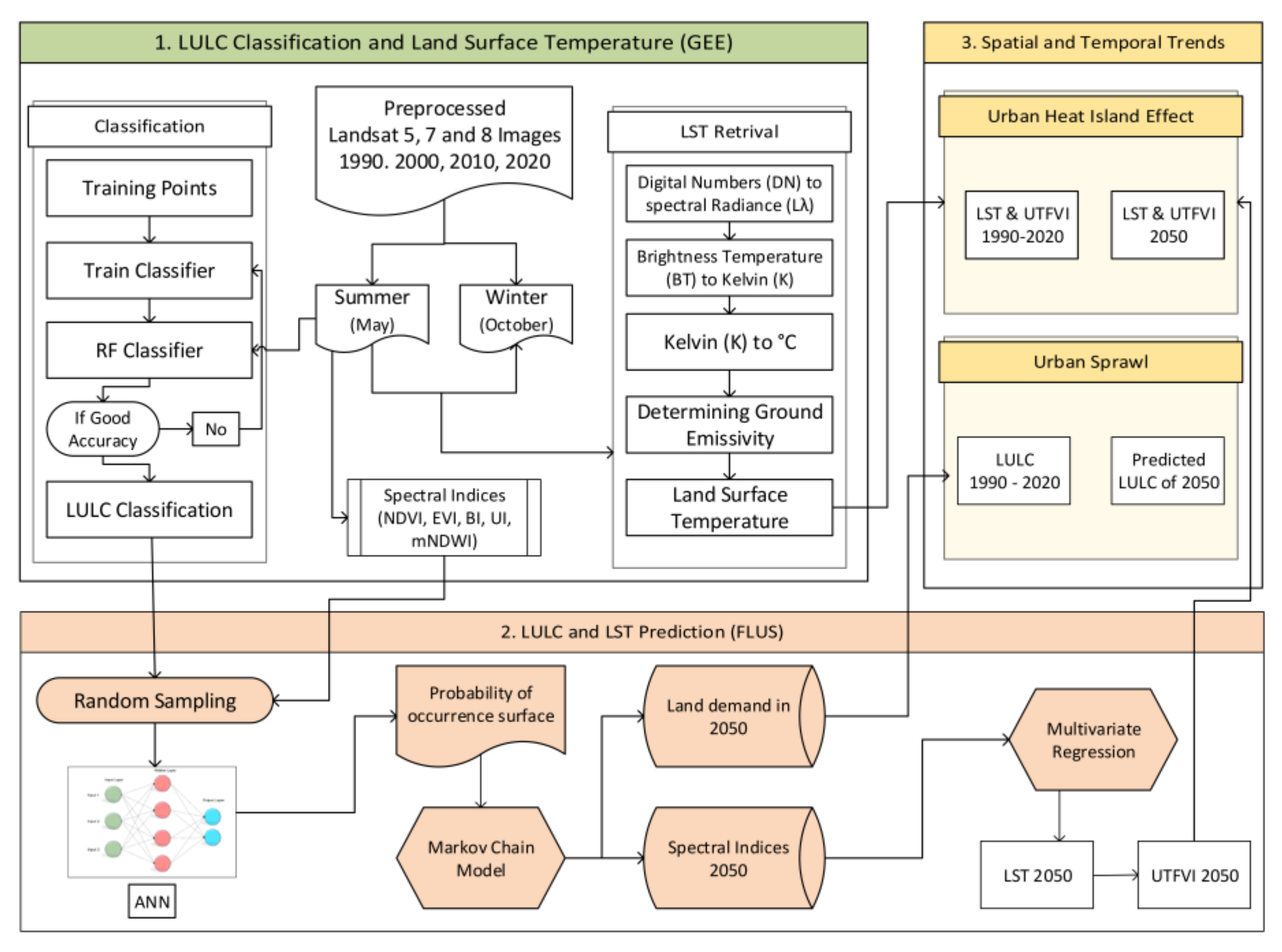This future prediction could have various implications for dealing with several challenges linked to climate, environmental processes, land use problems, food security, and urban planning and management [1,12]. Recently, various models have been introduced to predict LULC patterns, such as empirical models, evolutionary models, SLEUTH, cellular automaton (CA)-Markov chain model (MCM), agent-based models, artificial neural network/multiple perceptron neural network-based models (ANN/MLPNN), and future land use simulation model (FLUS) [1,4,8,10,11,12]. Most of the mentioned models, such as SLEUTH, empirical models, ANN/MLPNN, and CA-based MCM, require high training data inputs, huge computation power and time, and usually provide no graphical user interface (GUI) for visual interaction between user and model. Furthermore, most of the models, such as MLPNN, require the user to convert all data into a software-specific format which is inconvenient. In contrast, the FLUS model has a user-friendly GUI, requires spatial drivers (elevation, slope, distance to roads, towns, rivers etc.), and integrates top-down system dynamics (SD) and bottom-up CA models for improved and accurate LULC simulations [12]. This model is more efficient than the existing ones because it takes into account both anthropogenic and natural environmental effects [12]. Additionally, due to its interactive coupling mechanism between SD and CA models, it is much easier to operate—making it robust (see Section 2.4. for details).

An urbanization-led decrease in vegetation and an increase in impervious surface results in immense heat, and cities might experience the urban heat island (UHI) effect. UHI is a phenomenon when the observed surface temperature of core urban cities is higher than the surrounding sub-urban/rural areas [13,14], and has strong associations with public health-related issues [15]. Though there is no prominent boundary differentiating urban from nearby rural areas, a temperature difference is observed and well-documented around the world [8]. The design of cities, impervious surfaces such as roads, tall buildings, and non-vegetative regions (e.g., sandy or barren) within cities are primarily responsible for the UHI effect. The primary contributors to urban warming are a rise in short-wave radiation captivation, heat storage, human-induced heat generation, and reduced evaporation rate [8]. Earth observation data (EOD) are proven to be useful to understand the urbanization process and associated environmental effects. The use of EOD to evaluate UHI and its effects on spatial distribution, urban vulnerabilities, and health-related risks are widely published globally [16,17,18]. To evaluate the influence of UHI, the urban thermal field variance index (UTFVI) is usually employed [19]. Hence, exploring spatial-temporal heterogeneities in UTFVI could provide progressive opportunities to advance our understanding of UHI effects in cities.

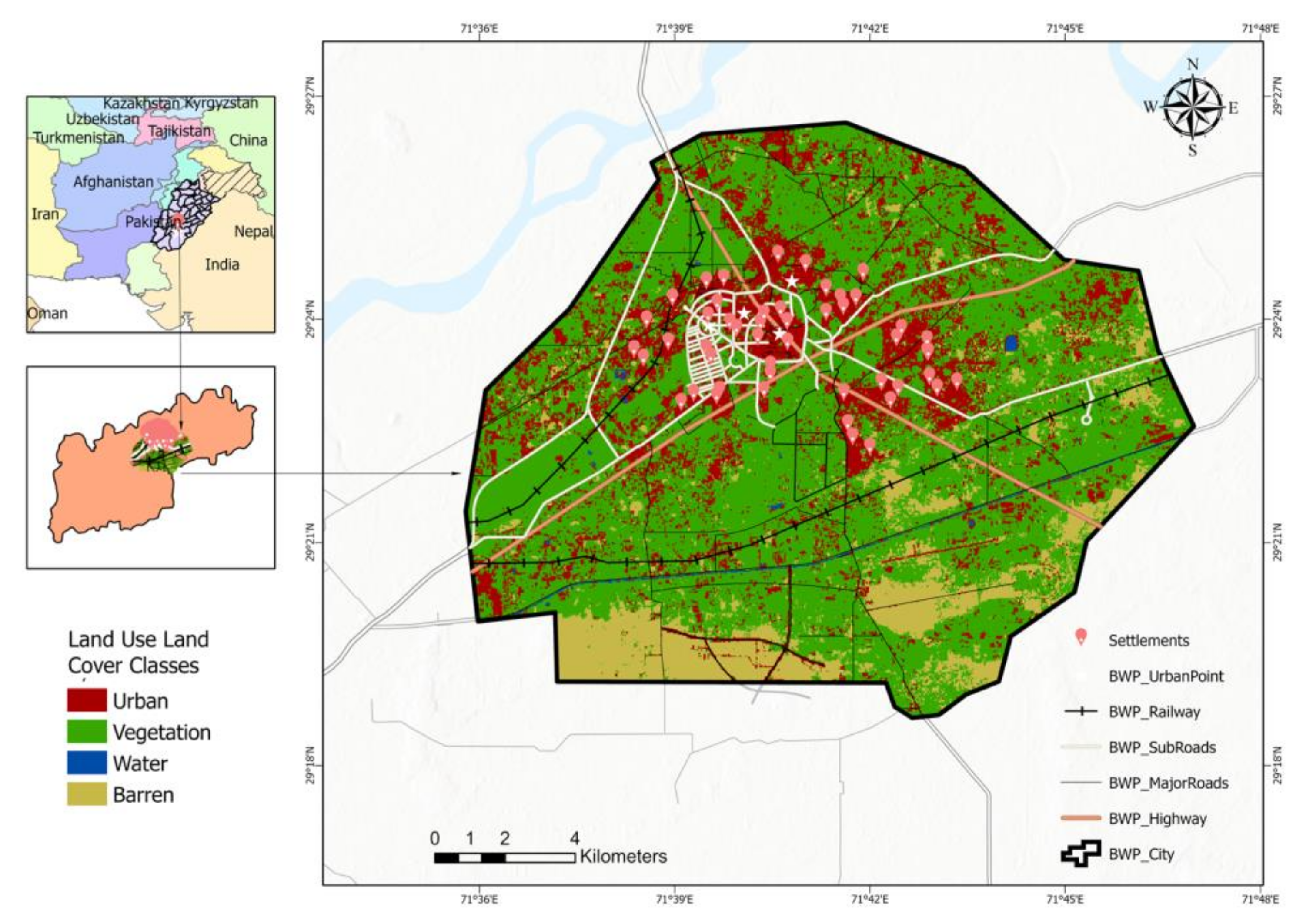
In the last five decades, Pakistan has faced rapid urbanization in its metropolitan cities [20]. Punjab, the largest province concerning population and agricultural productivity, has undergone some noticeable changes in its urban areas. Many researchers [21,22,23,24,25,26] have studied the LULC patterns of an individual or multiple cities of Punjab, but most of this research fails to address either future urban sprawl scenarios or its integration with climatic conditions. Furthermore, while such assessments are rare to find in Pakistan, those that are available mostly focus on the top metropolitan cities (i.e., Lahore, Karachi, and Faisalabad) despite their smaller city area and already highly urbanized nature [20,21,27]. Even though some localized studies are available in other cities, they solely address the LULC changes and are exclusive of future prediction, as well as investigating associations between LULC and climatic conditions. This situation represents a significant information gap for other rapidly urbanizing regions. Such a lack of research focus hinders informed planning and policy production in these rapidly urbanizing areas. Hence, to fill this knowledge gap, the present study integrates geo-information modelling techniques (i.e., cloud-computing-based Google Earth Engine, geographic information systems, remote sensing, and CA-based MCM, etc.), to evaluate historical and future trends and patterns in urban growth in Bahawalpur, one of the largest (third largest according to city area), populated (ranked 6th), and fastest-growing cities in Punjab [28]. Additionally, we evaluate the spatial-temporal UHI effect using the urban thermal field variance index (UTFVI) during 1990–2020. While urban sprawl monitoring and prediction, along with its association with urban climatic conditions, are essential to long-term efficient urban planning [29,30], evaluations as such can progressively assist urban planners, mitigation and adaptation professionals, and decision-makers in designing appropriate action plans for optimized land and resource allocation to make livable cities [31].

2. Materials and Methods

2.1. Study Area

Bahawalpur is the largest district of Punjab with respect to its geographical area. It consists of five subdivisions (called tehsils), including Bahawalpur, Ahmadpur East, Yazman, Khairpur Tamewali, and Hasilpur. Bahawalpur city has undergone massive urbanization in the last four decades [28]. According to the 2017 census, population-wise, Bahawalpur stands at 11th and 6th place in Pakistan and Punjab, respectively [32]. In the last half-century, the city’s population increased from 135, 263 persons in 1972 to 762, 111 persons in 2017, with an annual growth rate of 3.3%, far above the national average of 2.4%. The location of the study area is 29.3544° N and 71.6911° E, as shown in Figure 1. Due to its geographical location and physiological settings, the climate in Bahawalpur in the summer season is scorching and dry, while in the winter, the weather is dry and chilly. The maximum temperature climbs to 48 °C, while the minimum temperature drops to 7 °C [28,33,34].

2.2. Research Methods

For this study, the overall workflow is divided into three tasks. The first task emphasizes the classification of LULC and the retrieval of LST using a cloud computing-based platform—Google Earth Engine (GEE). This information is later used for change detection in LULC and UHI evaluation. The second task is based on the prediction of LULC using FLUS via integrating several physio-environmental datasets to explore the future urban growth in the study area. The last task is to employ geographic information system (GIS) techniques along with other statistical methods to perform spatial-temporal quantifications (Figure 2). All these tasks are detailed in the following sections.

2.3. Data Acquisition, Preprocessing, Classification and Change Detection

2.3.1. Data and Preprocessing

To begin with, data from Landsat achieves are used to study the spatial-temporal trends in LULC during the past 30 years (1990–2020). The data are freely available and integrated with the GEE data catalogue with a processing level of tier-1 for Landsat-5 Thematic Mapper (TM), Landsat-7 Enhanced Thematic Mapper Plus (ETM+), and Landsat-8 Operational Land Imager (OLI) [35]. For this study, we use Landsat-5 TM data for 1990 and 2010, Landsat-7 ETM+ for 2000, and Landsat-8 OLI for 2020. For 2010, Landsat-7 ETM+ data is also available, but we avoided using it due to the scan line error [36]. The Landsat-7 ETM + sensor has been collecting and delivering data since June 2003, despite strips induced by the Scan Line Corrector (SLC) malfunction. Although many approaches are available to overcome the effect of strips, Landsat-5 TM is preferred for 2010 to avoid distortion in results. Preprocessing steps are applied to each image individually. The preprocessing starts with masking clouds, heavy aerosols, and cloud shadows from each image. The resulting images are then clipped to the study area shapefile. The details on Landsat image acquisition and its sources are given in

Table 1. Datasets used in this study along with their sources.

Name	Description	Resolution	Bands	Date	Air Temp. (°C)	Source
Landsat-5 TM Tier-1	Collection 1, Tier-1 SR data used for LULC and LST	30 m	B1, B2, B3, B4, B5, B6, B7	05-1990	37.25	https://developers.google.com/earth-engine/datasets/catalog/landsat-5 (accessed on 1 March 2021)
				11-1990	27.85
				05-2010	36.94
				11-2010	29.5
Landsat-7 ETM+ Tier-1	Collection 2, Tier-1 SR data used for LULC and LST	30 m	B1, B2, B3, B4, B5, B6, B7	05-2000	37.54	https://developers.google.com/earth-engine/datasets/catalog/LANDSAT_LE07_C02_T1_L2 (accessed on 1 March 2021)
				11-2000	29.94
Landsat-8 OLI Tier-1	Collection 2, Tier-1 SR data used for LULC and LST	30 m	B2, B3, B4, B5, B6, B7	05-2020	36.2	https://developers.google.com/earth-engine/datasets/catalog/LANDSAT_LC08_C02_T1_L2 (accessed on 1 March 2021)
				11-2020	27.8
SRTM Digital Elevation	Elevation Data used as a variable for LULC prediction	30 m	Elevation	02-2000		https://developers.google.com/earth-engine/datasets/catalog/USGS_SRTMGL1_003?hl=en (accessed on 1 March 2021)
Roads, Canals, Settlements	Distances to roads, canals and settlements were evaluated for LULC prediction			07-2020		https://data.humdata.org (accessed on 1 March 2021)

. After preprocessing, classification is performed individually for each year using the Random Forest (RF) algorithm in GEE for faster computation—additional details can be seen in [4,8].

2.3.2. LULC Classification and Change Detection

For Landsat-5 and 7, bands 1-5 and 7 are used, whereas for Landsat-8, bands 1-6 are used. Comprehensive background information on the spectral range and specifications of each band is provided by [37]. Random forest (RF), a type of machine learning (ML) algorithm, is used to perform a supervised classification in GEE. Previously, for LULC mapping, the RF algorithm has outperformed some of the most dominant classification approaches like parametric techniques (maximum likelihood) and non-parametric techniques (decision trees, neural network) [38,39]. Furthermore, in previous literature, RF outperformed other classifiers with an accuracy greater than 80% [40,41]. Therefore, this study utilized the RF algorithm for LULC classification. After parametric tuning, the best-suited number of trees value for RF is set to 115. In RF-based classification, four land use classes are chosen for our study area. The details of the classes are given in

Table 2. Description of land use types used in this study.

LULC Class	Description
Urban	Impervious surface, central business district, high and low-density residential area with low vegetation fraction
Vegetation	Agricultural areas, forest, rangeland, sparse vegetation, intercity green spaces, fallow land
Water	Surface water bodies like natural or artificial wetlands, rivers, canals, lakes, and reservoir
Barren	Vegetation fraction less than 10%, sandy, desert, rocky area

. Land cover classes are identified and differentiated using GEE visual image interpretation techniques (tone, texture, and pattern), spectral signatures/responses, and mosaicked Google high-resolution background satellite images [42]. Around 50 polygons samples are taken for each class out of which 70% are utilized for training the RF classifier, while the rest of the 30% are used to assess the accuracy of the created land cover maps.

The LULC results are reliable only when they meet certain quality checks via different accuracy assessment metrics. Kappa coefficient (K) and overall accuracy (OA) are the two metrics widely used to evaluate the performance of LULC classifications [4,22]. Thus, we derive the error matrix for each LULC classification, which is further used to assess K and OA. The Kappa coefficient (K)—also known as Cohen’s kappa coefficients—is a statistical method that is used to check the reliability of categorical items as it indicates the extent of agreement between frequencies of two different variables at different intervals [43]. It is evaluated using the following [44]:

$$\mathrm{K}=\frac{p_o-p_e}{1-p_e}$$

(1)

where p_o = observed agreement, and p_e = expected agreement.

Similarly, the OA is calculated by summing the correctly classified pixels and dividing them by the total pixels given as [4]:

$$OA=\frac{t_p+t_n}{t_p+t_n+f_p+f_n}$$

(2)

where t_p = true positive, t_n = true negative, f_p = false positive, and f_n = false negative.

After obtaining reliable accuracies, change detection is performed to evaluate the changes in different land-use types over the years. Change detection using a per-pixel approach is a postprocessing technique that analyzes changes in each pixel value over different time intervals [37]. This technique is preferred over conventional (preprocessing-based) ones as it reduces sensor, atmospheric, and environmental effects—provides more information on spatial conversions of different land-use types [5]. To perform the change detection, the Semi-Automatic Classifier Plugin inside Quantum GIS (QIS) (freely available at https://qgis.org/, accessed on 1 April 2021) is used.

2.4. Simulating Future LULC Using the FLUS Model

In the second task, the Future Land Use Simulation model (FLUS) is used to predict change in land use types using the top-down SD and bottom-up CA methods. Following the model guidelines (available at: http://www.geosimulation.cn/flus.html, accessed on 1 April 2021), four variables including elevation, slope, distance to roads, and distance to settlements are used to simulate future land use patterns. The elevation and slope are derived from the digital elevation model (DEM) obtained from the shuttle radar topography mission (SRTM) provided by the National Aeronautics and Space Administration (NASA) [45].

The FLUS model is originally developed by Liu et al. [12]. It uses a spatial simulation method based on a CA model and trains an ANN model to create a land-use probability-of-occurrence (PO) surface. The links between historical land use and various driving factors are defined using an ANN. Changes in land-use distribution are guided by the PO surfaces obtained from the ANN. The CA module’s total likelihood of land-use type is adjusted according to the total quantity of that land-use area in the scenario using a self-adaptive inertia coefficient [46]. The simulation process is separated into multiple periods, and the bottom-up CA model and the top-down urban demand forecasting model are strongly coupled during the time series under consideration [47]. The multiple CA allocation model is established to simulate the future spatial pattern under the given land-use demands determined by the SD model.

First, the CA simulation is carried out in two steps: (1) an ANN is utilized for training and assessing the chance of each land-use type occurring on a specific grid cell; and (2) sophisticated self-adaptive inertia and competition mechanism are devised to address competition and interactions among the various land-use types. Second, the SD model is used for the computation of future land use scenario demands under multiple factors including but not limited to socio-economic and natural environmental factors at national/regional scales. Self-adaptive inertia and competition mechanism are developed within the CA model to process the complex competitions and interactions among the different land-use types [12,48]. The aggregate probability of all land use types at each grid cell is estimated in these two steps, and the dominant land use type is assigned to the cell during the CA iteration. Depending on their combined probability and the roulette pick, a specific land grid remains the present land-use type or evolves into another type during the allocation process.

2.5. LST Retrieval through Landsat Thermal Bands

The third part used Landsat-derived land surface temperature (LST) to analyze UHI in Bahawalpur city. For this purpose, LST was taken from summer (May) and winter (November) months satellite images individually for each year. The mean of each image in each seasonal month was taken to provide a more representative condition of the study area [1]. Seasonal land surface temperatures (LST) are calculated for each year using the Landsat TM and ETM+ (B6) and Landsat OLI/TIRS (B10) thermal bands. For each year, Landsat images in May (summer) and November (winter) are taken and their per-pixel mean values are utilized to produce two individual images of summer and winter, respectively. Landsat 8 (OLI/TIRS) imagery has two thermal bands (10 and 11), but only band 10 is used for the LST estimation because of its more accurate results [49]. Equations (3)–(5) are used to convert digital numbers (DN) into LST as previously used by [50]. Firstly, the DN values of each pixel are converted into radiance values (L_λ) using the following:

$$L_{\lambda }=\left(\frac{L_{max\lambda }-L_{min\lambda } }{QCA{L}_{max}-LQCA{L}_{min}}\right)+L_{min\lambda }$$

(3)

where L_maxλ is the highest radiance value, L_minλ is the lowest radiance value, QCAL_max is the highest quantized adjusted pixel value (consistent to L_maxλ in DN (value = 255)), QCAL_min is the lowest quantized adjusted pixel value (consistent to L_minλ DN (value = 01)).

All the values information used in Equations (3)–(5) are taken from the metadata files that come along the Landsat images. The radiance values are then converted into a surface brightness temperature given as:

$$T_B=\left(\frac{K_2}{\ln \left(\frac{K_1}{L_{\mathsf{\lambda }}}+1\right)}\right)-273.15$$

(4)

in which K₁ and K₂ are the constants, and their values are available on the United States Geological Survey (USGS) website (https://www.usgs.gov/, accessed on 1 April 2021).

After estimating the at-surface brightness temperature T_B, we compute the pixel-based land surface emissivity (ε). To calculate the value of emissivity, we use the pre-defined calibrated values for different Landsat missions along with the particular region’s normalized difference vegetation index (NDV) as used in recent research [51,52]. The LST is computed using Equation (5) in which T_B is applied with an emissivity correction (ε):

$$T_S=\frac{T_B}{\left[1+\left[\frac{\mathsf{\lambda }{T}_B}{p}\right]\ln \mathsf{\epsilon }\right]}$$

(5)

where T_S is the per-pixel LST value, λ is the wavelength of emitted radiance (value = 11.5 µM), and p is equal to 1.438 × 10^−2mk.

The above procedure is followed to evaluate LST for each season image as mentioned in Table 1. The derived LST is then used to evaluate the spatial-temporal patterns and trends, if any, in the study area over the last three decades (1990–2020). In addition, LST is further used to assess UHI and UTFVI, which is used to map heat stress-affected areas in the study area.

2.6. Simulating LST for 2050

Land cover indices or spectral indices are popular for predicting LST as they provide valuable information about the spectral reflectance of the features of interest for the bands used. In literature, the use of the normalized difference vegetation index (NDVI), modified normalized difference water index (mNDWI), enhanced vegetation index (EVI), bare soil index (BI), and urban index (UI) is supported for LST predicting as these contribute to mapping the strength of surface temperature [1,21]. The details of spectral indices used in this study are given in

Table 3. Details of spectral indices used in this study for LST prediction.

Index	Name	Formula	Justification
NDVI	Normalized Difference Vegetation Index	$\frac{\left(NIR-Red\right)}{\left(NIR+Red\right)}$	[53]
mNDWI	Modified Normalized Difference Water Index	$\frac{\left(Green-NIR\right)}{\left(Green+NIR\right)}$	[54]
EVI	Enhanced Vegetation Index	$\frac{\left(NIR-Red\right)}{NIR+6\times Red-7.5\times Blue+1}$	[55]
BI	Bare Soil Index	$\frac{\left(SWIR1+Red\right)-\left(NIR+Blue\right)}{\left(SWIR1+Red\right)+\left(NIR+Blue\right)}$	[56]
UI	Urban Index	$\frac{\left(SWIR2-NIR\right)}{\left(SWIR2+NIR\right)}$	[57]

Where NIR = near infrared band, Red = red band, Green = green band, Blue = blue band, SWIR1 = shortwave infrared-1 band, SWIR2 = shortwave infrared-2 band.

. First, these indices are evaluated for the 2010 and 2020 summers using the same satellite images used to derive LULC maps. Then, correlation analysis is performed to evaluate the relationship between different factors contributing to LST (Figure 3). The correlation showed that a significant bivariate correlation exists between various spectral indices and LST. Given that, multiple regression analysis is performed using the 2020 summer LST as the dependent variable and spectral indices (NDVI, EVI, BI, and UI) for the 2020 summer as independent variables. The purpose of regression analysis is to evaluate the regression equation, which can then be used to predict spectral indices for 2050.

In Figure 3, it is observed that some spectral indices are highly correlated with each other (i.e., NDVI with EVI, and BI with UI). Therefore, to avoid the multicollinearity effect in the regression model, only EVI and BI are used as predictors in the regression equation. The resulting regression equation (Equation (6)) with reasonable variance is then used to predict LST for 2050. For predicting 2050 LST, first BI and EVI are predicted for 2050 using the CA-Markov model in FLUS again. Initially, 2010 and 2020 summer BI and EVI rasters are used, and a probability of change matrix is created. Then, based on the probability of change in that decade, the CA-Markov model is run to generate BI and EVI for 2050. In the last, both BI and EVI are inserted in the regression model to get the LST for 2050. Here, since BI and EVI spectral indices have 30 m spatial resolution, the resultant predicted 2050 LST has the same spatial details of 30 m resolution.

$$LST\_2020\_s=34.125+(54.44\times \left(BI\_2020\_s)\right)+\left(19.83\times \left(EVI\_2020\_s\right)\right)$$

(6)

2.7. UTFVI Estimation and Its Spatial-Temporal Heterogeneities

Urbanization is the major contributor to changes in LULC and also the driver of UHI. Previously, UHI has been evaluated by comparing temperature in urban areas with its neighboring rural areas [8]. UHI phenomenon has gained importance in recent years due to its pronounced effects in metropolitan cities and consideration in urban designs to develop a more livable environment in cities [58]. Previously, many researchers have used different techniques to calculate the intensity of UHI specifically in urban and near urban areas [1,8,59,60]. Remote sensing (RS) techniques have been proven to analyze data continuously and cost-effectively. Using RS techniques, UHI can be monitored continuously with the help of infrared satellite data. Instead of just point readings, the RS-based UHI will show the intensity of heat stress over large geographical areas. According to previous literature [59], the UHI is directly linked to different LULC classes and also to the geographical distribution of vegetation cover. By using RS techniques, the UHI is calculated independently in urban and rural areas following Faisal et al. [1].

A normalized method is adopted to compare UHI due to observed variations in LST of different seasons within a year. This is given as Equation (7):

$$UH{I}_N=\frac{T_s-T_m}{T_{Std}}$$

(7)

where $UH{I}_N$ is the normalized UHI, T_s is the LST, T_m is the mean LST of the study area, and T_Std is the standard deviation LST of the study area.

After computing the UHI, we use the UTFVI to describe its effect. The UTFVI is a quantitative measure to explain UHI in terms of thermal comfort level in a city and is among the most widely used thermal comfort indices [16,61]. The index value is quantitatively calculated using the formula given in Equation (8):

$$UTFVI=\frac{T_s-T_m}{T_s}$$

(8)

where the variables are similar to Equation (7).

The UTFVI is computed for both summer and winter seasons for each period (1990, 2000, 2010, and 2020), and maps are produced to provide spatial references on geographical disparities. This approach is particularly helpful in understanding the distribution of urban thermal comfort across space and time, allowing relevant authorities to take appropriate measures via informed decision-making. To comprehend the large values, we bin the UTFVI into six different classes [16]. The ranges of these six different values as noted in [62] are given in

Table 4. Reference UTFVI threshold values used for categorizing six UTFVI classes.

UTFVI Threshold Value	UHI Strength
$<0$	None
$0.000–0.005$	Weak
$0.005–0.010$	Middle
$0.015–0.015$	Strong
$0.015–0.020$	Stronger
$>0.020$	Strongest

. Besides this, we also predicted UTFVI for 2050 using the 2050 LST derived earlier. By applying the same Equations (7) and (8) UTFVI based on 2050 LST at 30 m spatial resolution is prepared.

3. Results

3.1. LULC Classification and Change Analysis

The results from the RF algorithm-based LULC classification between 1990 to 2020 with a 10-year gap interval are presented in Figure 4. It is noticeable that the urban area expanded over three decades, whereas a decrease in barren land is observed. From a broader perspective, it is evident that most of the vegetation land was converted into urban land, and barren land was transitioned primarily into vegetation and urban. To verify the derived LULC information, an accuracy assessment is performed, and the results are detailed in

Table 5. Accuracy assessment of resulting classified LULC maps.

Year	OA	Kappa
1990	0.96	0.95
2000	0.94	0.92
2010	0.92	0.9
2020	0.91	0.89

. The results show that OA is more than 0.91 in all years with K greater than 0.89, which shows an excellent agreement between actual and classified pixels.

Once the reliability and accuracy are confirmed, the area of different land use classes is evaluated statistically. Area-wise distribution of LULC classes is shown in

Table 6. Area estimation of different LULC classes from 1990 to 2020.

LULC Classes	1990		2000		2010		2020
	Area (ha)	Area (%)	Area (ha)	Area (%)	Area (ha)	Area (%)	Area (ha)	Area (%)
Urban	2142.05	11.48	2645.44	14.18	3329.16	17.85	4071.59	21.83
Vegetation	12,961.48	69.48	13,195.64	70.74	13,222.68	70.88	12,104.94	64.89
Water	41.17	0.22	8	0.04	97.96	0.53	95.42	0.51
Barren	3510.25	18.82	2805.87	15.04	2005.17	10.75	2383.01	12.77

. It is observed that the vegetation class is the most prominent in the study area, with the largest area as compared to other classes. A decreasing trend is observed in the area of barren land as it decreased from 3510.25 ha to 2383.01 ha between 1990–2020. On the other hand, the urban class area increased from 2142.05 ha in 1990 to 4071.59 ha in 2020.

3.2. Change Detection Analysis

To further investigate the area-wise transition per decade, we perform change detection and the results are shown in

Table 7. LULC classes area percent change and overall change from 1990 to 2020.

LULC Classes	1990–2000		2000–2010		2010–2020		1990–2020
	MC (ha)	PC (%)	MC (ha)	PC (%)	MC (ha)	PC (%)	MC (ha)	PC (%)
Urban	503.39	23.5	683.72	25.85	742.43	22.3	1929.54	90.08
Vegetation	234.16	1.81	27.04	0.2	−1117.74	−8.45	−856.54	−6.61
Water	−33.17	−80.57	89.96	1124.5	−2.54	−2.59	54.25	131.77
Barren	−704.38	−20.07	−800.7	−28.54	377.84	18.84	−1127.24	−32.11

where MC = magnitude of change = vf − vi, PC = percent change = (vf − vi)/(vi × 100), vf = final year land use type area, vi = initial year land use type area.

. It is observed that urban areas experienced a rapid increase of 1929.54 ha (90.08%) from 1990 to 2020. On the contrary, vegetation and barren classes show decreasing trends with −856.54 ha (−6.61%) and −1127.24 ha (−32.11%) during the study period. To assess the contribution of several LULC types to urban growth, we further evaluated different land-use transitions into urban (Figure 5). The spatial references of these transitions are presented in Figure 5a. It is evident that the surrounding areas of the city are engulfed to facilitate its urban growth. The Sankey diagram in Figure 5b represents the comparative transition of different land-use types in urban areas. It is evident that the largest contribution to urban growth is made by the vegetation areas (68.32%) followed by barren land (7.85%) and water (0.25%). This situation reflects the gravity of urban growth and vegetation loss, which might result in higher temperatures in the study area due to an increase in impervious surface.

3.3. LULC Prediction and Validation for 2020

This study utilizes the top-down SD model and bottom-up CA integrated into the FLUS model to simulate future LULC patterns. To inspect the performance of the FLUS model, the LULC of 2000 and 2010 is used to initially predict the LULC for 2020. For that, the SD model is used to derive transition potential and land use demand for the year 2020 and multiple CA-based ANN model is used for land use simulation in 2020. The transition potential used for simulating land use demand in 2020 is shown in

Table 8. Markov transition probability for simulated 2020 LULC map, shows alternations between different LULC classes.

LULC Classes	Urban	Vegetation	Water	Barren
Urban	1	0	0	0
Vegetation	0.150807	0.83949	0.006483	0.003221
Water	0.327434	0.646018	0.026549	0
Barren	0.033848	0.278505	0	0.683871

. The simulated LULC for 2020 is prepared and is shown in Figure 6a.

The performance of simulated LULC is tested by comparing area-wise statistics of simulated LULC with actual 2020 LULC. Furthermore, the Chi-square test is performed to check the performance of prediction results. The details of the Chi-square test are shown in

Table 9. Simulated 2020 LULC map assessment based on actual and predicted LULC patterns.

Chi-Square Test
LULC Class	Area (ha) of LULC Classes in 2020	Area (ha) of LULC Classes in Predicted 2020	Percent Wise Area of Actual LULC 2020 (O)	Percent Wise Area of Predicted LULC 2020 (E)	(O − E)²/(E)
Urban	4071.59	3918	21.83	21	0.0328
Vegetation	12,104.94	12,309	64.89	65.99	0.0183
Water	95.42	92	0.51	0.49	0.0008
Barren	2383.01	2335	12.77	12.52	0.005
Total	18,654	18,654	100	100	0.0569

Note: $x^2=\sum \frac{{\left(\mathrm{O} - \mathrm{E}\right)}^2}{\left(\mathrm{E}\right)}=0.0569$; degree of freedom = 3 where O and E represent the area of the particular LULC class used for validation.

.

However, a problem associated with the Chi-square test as previously reported by Vinayak et al. [4], is that it does not validate the spatial distribution of various land-use patterns. To overcome this problem, four kappa matrices were derived namely k_no, k_standard, k_location, and k_{location strata} [63]. The calculated values of Kappa matrices are given in

Table 10. Resultant Kappa scores for the assessment of simulated LULC of 2020.

Type of Kappa Coefficient	Kappa Score of Simulated LULC for 2020
$k_{no}$	0.85
$k_{standard}$	0.75
$k_{location}$	0.70
$k_{location strata}$	0.94

and all values are greater than 0.7. The values of Kappa show that the simulation model and its spatial patterns are accurate and can be used for future LULC simulations.

3.4. Predicting LULC for the Year 2050

The LULC of 2010 and 2020 is used to derive transition potential for 2050, shown in

Table 11. Markov transition probability for predicted 2050 LULC map, shows alternations between different LULC classes.

LULC Classes	Urban	Vegetation	Water	Barren
Urban	1	0	0	0
Vegetation	0.213969	0.744606	0	0.03641
Water	0.274707	0.355109	0.948409	0.021776
Barren	0.090291	0.402279	0	0.804489

. The transitional potential (Table 11) is then used to predict LULC patterns for 2050. The predicted LULC for 2050 is shown in Figure 6b, whereas Figure 6a shows LULC in 2020. From a broader perspective, it is evident that urban areas are expected to increase rapidly at the expense of agriculture and barren lands (Figure 7).

To further investigate the changes in the predicted 2050 LULC, area-wise change detection is performed (

Table 12. LULC change analysis from 2020 to 2050.

LULC Class	Area in 2020	Area in 2050	Total Change	Percent Change
	(ha)	(ha)	MC (ha)	(%)
Urban	4071.59	6103	2031.41	49.89
Vegetation	12,104.94	10,292	−1812.94	−14.98
Water	95.42	136	40.58	42.53
Barren	2383.01	2124	−259.01	−10.87

). The results show that among LULC classes, the urban class is expected to experience the highest increase of 2031.41 ha (49.89%), whereas vegetation and barren classes have experienced a decrease of −1812.94 ha (−14.98%) and −259.01 ha (−10.87%), respectively. For urban sprawl assessment, only the urban class from each year (1990, 2000, 2010, 2020, and 2050) is taken and overlapped to produce a thematic map (Figure 7). Additionally, to visualize the state of urban sprawl in terms of impervious surface expansion, the major road layer is overlayed at the top, which highlights urban expansion taking place along roads-adjacent areas. Notably, the urban areas in 2050 are expected to increase more on the northeastern and southwestern sides of the study area and the urban growth is prominent along roadside areas.

3.5. LST Seasonal Variation over Bahawalpur

Seasonal LST is evaluated using GEE from 1990 to 2020 using Landsat missions. In summer (Figure 8a), the maximum surface temperature is observed in 2000 (57.21 °C), whereas the lowest temperature is noted in 1990 (32.21 °C). In the summer of 1990, most of the southeastern areas are highlighted as having high temperatures. In contrast, this strength decreases in the 2020 summer. This is primarily because, in 1990, high-temperature areas were barren (desert areas) which were converted into vegetation and urban areas in 2020 (Figure 4). Additionally, each year, the lower part of Bahawalpur city shows relatively higher LST compared to the central urban area. This is primarily because the lower part of Bahawalpur comprises desert and barren land with sparse or no vegetation, whereas the central urban areas have an impervious surface with green spaces. Similar trends are observed for winter LSTs (Figure 8b). Just like the summer LST, the highest temperature in winter is recorded for the year 2000 (48.67 °C), whereas the lowest is recorded in 1990 (26.47 °C).

3.6. Spatial-Temporal Heterogeneities in Urban Thermal Field Variance Index

The urban thermal field variance index (UTFVI) quantifies the quality of urban health and ecology and directly represents the degree of thermal comfort in urban areas—an indicator of urban livability. The values of UTFVI are categorized according to the strength of UTFVI defined by [62]. Figure 9 shows summer (a) and winter (b) distributions of UTFVI in the study area. Visually, in both seasons, the lower barren part of the study areas shows the strongest values of UTFVI, whereas the central part of the city (the core urban area) shows increasing strength in acceding order according to years. The areas for each UTFVI class and its percentage-wise statistics are presented in

Table 13. Area-wise distribution of UTFVI from 1990 to 2020. The % sign reflects the percent share of each class as compared with the total area.

UTFVI	Summer								Winter
	1990		2000		2010		2020		1990		2000		2010		2020
	Area (ha)	%	Area (ha)	%	Area (ha)	%	Area (ha)	%	Area (ha)	%	Area (ha)	%	Area (ha)	%	Area (ha)	%
None	654	3.49	743	3.97	684	3.65	428	2.28	2643	14.1	3595	19.18	2881	15.37	1586	8.46
Weak	3637	19.41	4420	23.59	2619	13.98	1908	10.18	4121	21.99	5033	26.86	4594	24.51	4153	22.16
Middle	3785	20.2	5142	27.44	2548	13.6	2979	15.9	2103	11.22	2044	10.91	2492	13.3	2328	12.42
Strong	3258	17.39	3097	16.53	3650	19.48	4286	22.87	3335	17.8	2277	12.15	2015	10.75	3300	17.61
Stronger	3498	18.67	2375	12.67	5081	27.11	6053	32.3	3958	21.12	2360	12.59	3896	20.79	4106	21.91
Strongest	3908	20.85	2964	15.82	4157	22.18	3086	16.47	2564	13.68	3431	18.31	2857	15.25	3268	17.44

. A decreasing trend in areas with lower UTFVI (none, weak and middle) whereas an increasing trend in areas with higher UTFVI strength (stronger, and strongest) is observed. To further investigate per-decade changes in seasonal UTFVI, change detection is performed (

Table 14. Percent change in UTFVI classes from 1990 to 2020.

UTFVI	Percent Change (%)						Overall Change (%)
	Summer			Winter			Summer	Winter
	1990–2000	2000–2010	2010–2020	1990–2000	2000–2010	2010–2020	1990–2020	1990–2020
None	36.02	−19.86	−44.95	13.61	−7.94	−37.43	−39.99	−34.56
Weak	22.13	−8.72	−9.6	21.53	−40.75	−27.15	0.78	−47.54
Middle	−2.81	21.92	−6.58	35.85	−50.45	16.92	10.7	−21.29
Strong	−31.72	−11.51	63.77	−4.94	17.86	17.42	−1.05	31.55
Stronger	−40.37	65.08	5.39	−32.1	113.94	19.13	3.74	73.04
Strongest	33.81	−16.73	14.39	−24.16	40.25	−25.76	27.46	−21.03

). The overall change results show that the none, weak, and middle classes show decreasing trends in both seasons except for summer in which a minor increasing trend of 0.07% and 10.7% is observed for weak and middle classes, respectively. It is evident that the areas showing the least UTFVI strength have gone through a massive decline in the last 30 years as the areas under the “none” class decreased by −39.99% and −34.56% in the summer and winter seasons, respectively. Most of these areas are converted into strong, stronger, and strongest classes of UTFVI with an overall percentage of 31.55% (winter), 73.04% (winter), and 27.46% (summer), respectively.

3.7. LST and UTFVI Simulation for 2050

LST derived through multivariate regression for 2050 (summer) is shown in Figure 10b while Figure 10a shows LST for 2020 summer. It is observed that the highest temperature reaches 53.09 °C (an increase of ~2 °C from 2020). Moreover, the city’s central areas were indicated by high temperatures similar to the surrounding desert areas in the southern part of the city. Using 2020 UTFVI as a baseline (Figure 10c), we compared the situation in 2050 using the predicted LST-based UTFVI (Figure 10d). It is observed that areas with minimum UTFVI effect are drastically reduced in 2050 compared to 2020. Other than that, areas with the strongest hold of UTFVI increased around the city’s central areas. To further quantify the UTFVI changes from 2020 to 2050, we performed statistical change detection between both UTFVI rasters (2020 and 2050), the results of which are shown in Figure 10e. This analysis verifies our previous deductions that the areas with minimum UTFVI effect are reduced in 2050 by −75.93%, and the areas with the strongest UTFVI effect increase up to +138.63% in 2050. In Figure 10e, the stronger zone of UTFVI shows an increase of +32.48% whereas other classes such as weak, middle, and strong shows a decrease of −7.12%, −1.95% and −22.8%, respectively.

3.8. Association between Predicted Land Use and UTFVI for 2050

In the last, to quantify the relationship between predicted UTFVI and LULC, we performed a geographical weighted regression (GWR) analysis using a 500 m² grid. For this, we designed two models, the first one being built up as explanatory and UTFVI as a dependent while in the latter one, vegetation being explanatory and UTFVI as a dependent. First, zonal statistics are performed and average UTFVI values are taken for each grid. Then, for each grid, the land-use class percentage per grid is evaluated. The resulting data are then employed in GWR models, and the results are shown in

Table 15. GWR spatial model output for model-1 and model-2.

GWR Output	Model-1 (Built-Up)	Model-2 (Vegetation)
R2	0.8316	0.8722
AdjR2	0.7873	0.8383
AICc	−6296.5043	−6501.9372
Effective Degrees of Freedom	597.8459	596.9261

and Figure 11. It is found that while the outcome of both models is reasonably good given the higher value of goodness-of-fit (R2), the AICc (an estimator of prediction error) for the model-1 is comparatively lower (i.e., ~6297 for model-1 versus ~6502 for model-2. Hence, it is evident that even though both the models can comprehend higher than 80% of the variance in the data, the larger difference between AICc values, which is higher than the commonly accepted threshold (cutoff value ≥ 3), indicates that built-up area-based model is more suitable. The spatial distribution of standard error and local-R2 is presented in Figure 11. It is observed that the general distribution of local-R2 for both models is similar and the performance of the model is better even for congested urban areas (darker blue shades).

4. Discussion

While monitoring LULC changes in the face of rapid urbanization is essential to the sustainable development of cities, the systematic evaluation of UHI through UTFVI provides insights regarding the comfort levels of a city—representing the livability in urban regions. Although urbanization is essential to economic growth, innovation, and development, unplanned and unsustainable growth in cities can potentially result in severe complications for residents [10]. This situation could potentially compromise the livability and sustainability of cities under climatic changes—highlighting short- and long-term challenges, respectively. Additionally, the UHI mitigation potential of urban vegetation is directly associated with the local surface type [8]. In this context, studies as such play a crucial role in informing urban policy and smart decision-making through empirical assessments of historical LULC change, its prediction based on spatial-environmental factors, and spatial-temporal urban comfort evaluation to cope with the UHI phenomenon. The United Nations projections show that global urban land will increase by 1.2 million km² by 2030 [4]. Since rapid urban growth in developing countries is much higher than the developed nations, it severely affects the spatial-environmental characteristics of urban areas resulting in localized issues such as increased LST-induced UHI effect and unsustainable land resource allocation/utilization [64]. To deal with this issue, assessments should be made not only to monitor and report historical trends and patterns of LULC changes but projections of urban sprawl via state-of-the-art techniques should also be established based on scientific backgrounds—such as demonstrated in this study. The results of LULC change during 1990–2020 and the projection of 2050 from this study are therefore useful information in the context of sustainable urban planning.

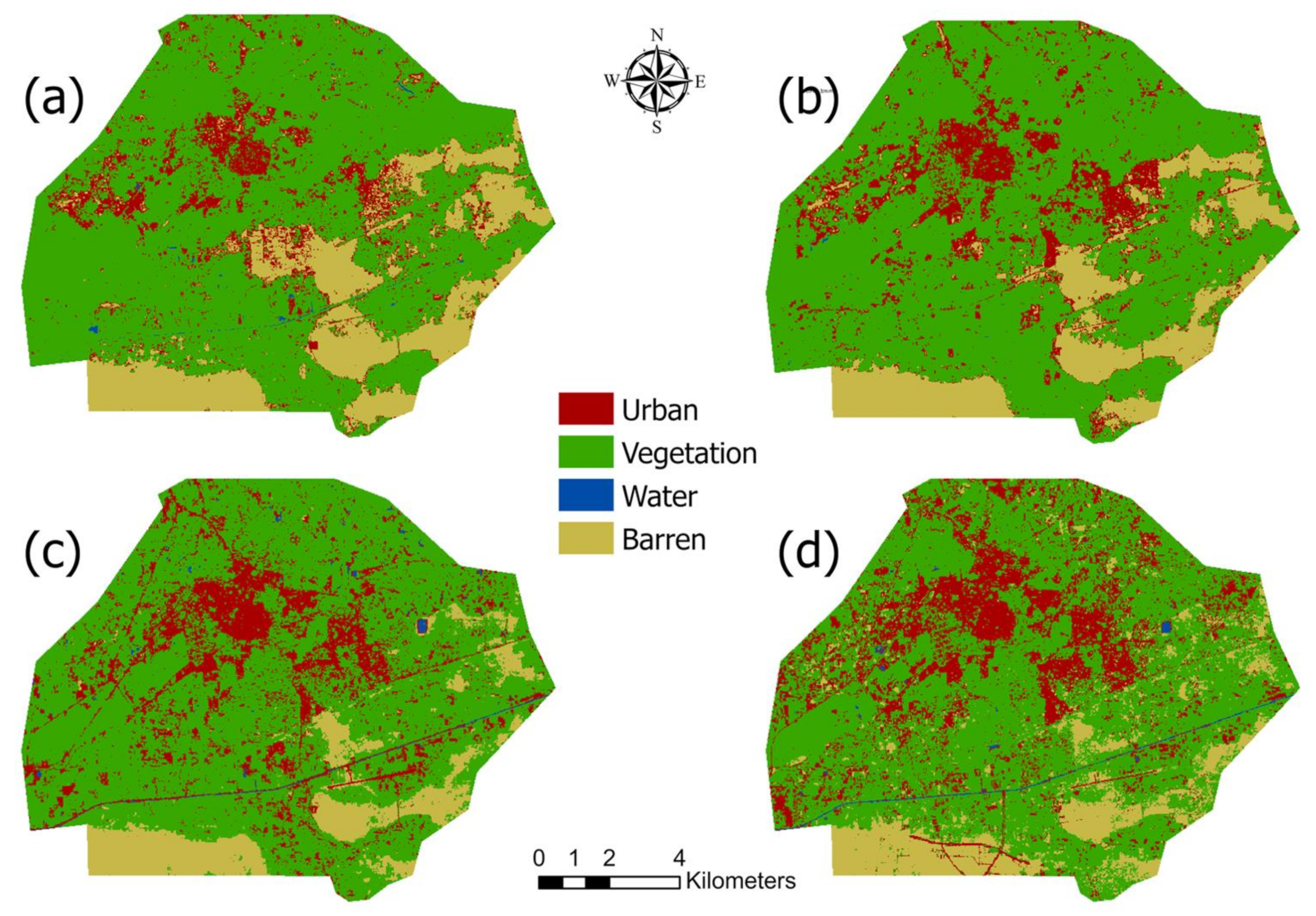
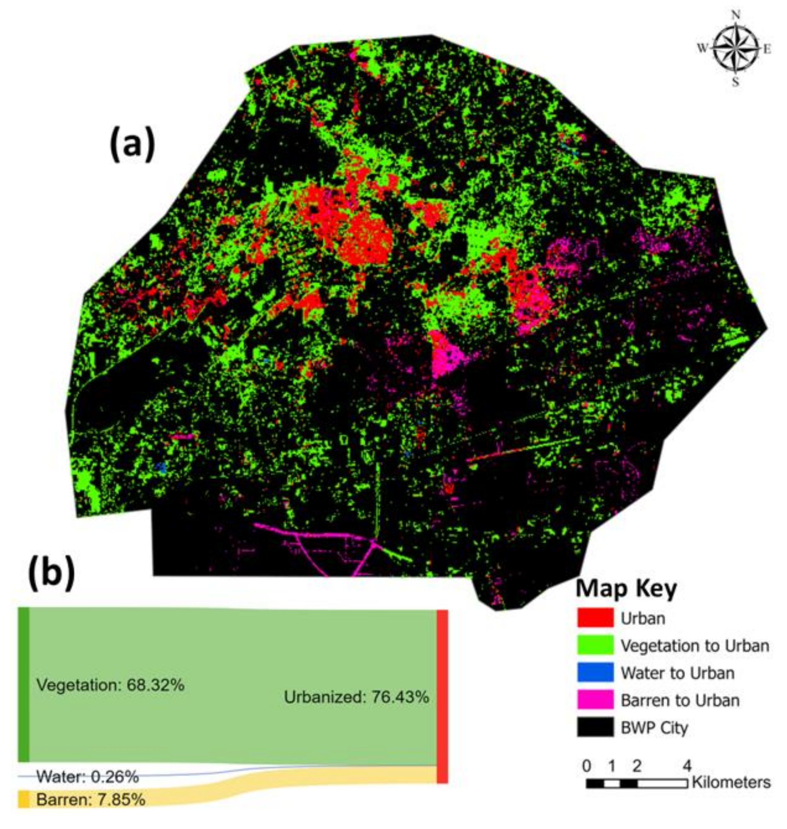
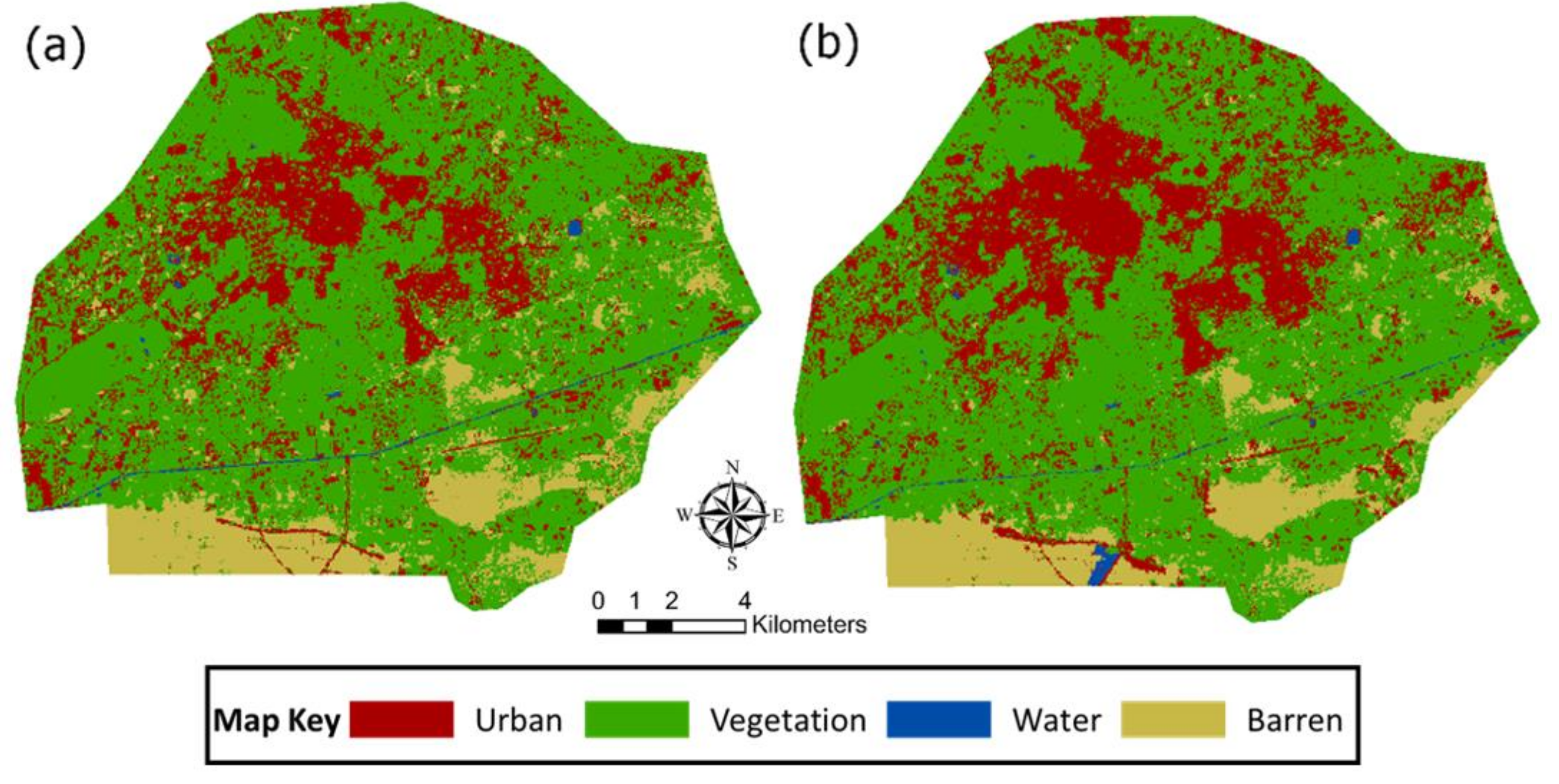
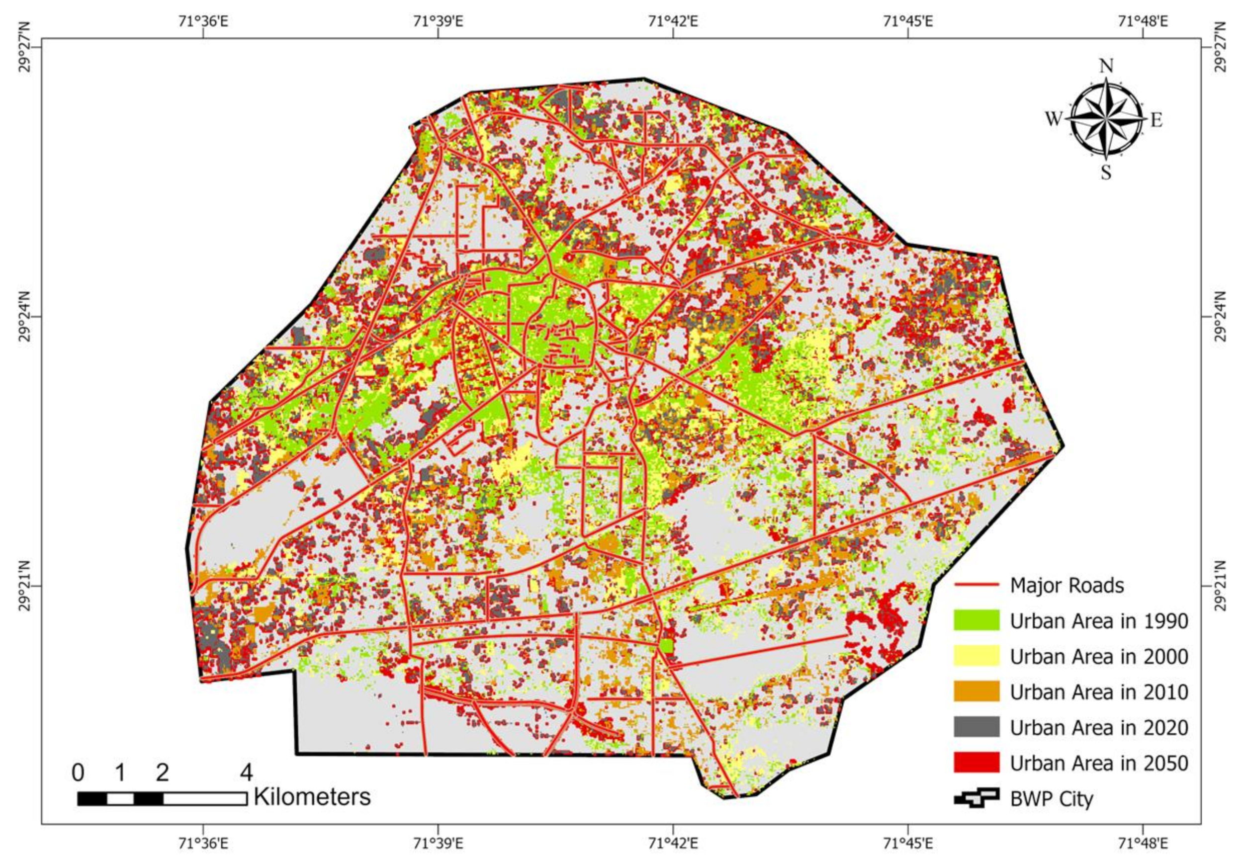
The increase in built-up areas at the cost of vegetation and bare land along with considerable urban growth prediction in our study (see Figure 5 and Figure 7) are consistent with studies conducted in other urban areas in Pakistan and beyond. For instance, Baqa et al. [27] reported an expected increase of 11.6% in Karachi’s urban areas —the largest city in Pakistan—by 2030. Similarly, Tariq and Shu [21] concluded that urban areas in Faisalabad—3rd largest city in Pakistan—would increase by 12.5% in 2048. Likewise, Kafy et al. [16] showed an expected 11% increase in urban areas of Cumilla, Bangladesh—another developing nation in Asia—in 2039. It is also notable that all these studies show rapid urban growth in respective cities. The same trends are found for our study area with a historical increase of ~90% during 1990-2020 and a ~50% expected increase in urban areas in 2050. It is noteworthy that the expected built-up increase in Bahawalpur is much higher than in Karachi and Faisalabad as mentioned above. For Karachi, the reason for the lower increment is their short-term prediction (2030 in Baqa et al. [27] versus 2050 in our case). Whereas, in the case of Faisalabad, the lower expected increase is due to the urban saturation in Faisalabad city (study area in Tariq and Shu [21]) as it is already highly urbanized, providing little room for further development. The possible reasons for historical rapid urban growth in Bahawalpur could be associated with population increase as the city faced a ~90% increase in population during 1998–2017. As a result, there has been a 51% increase in residential areas during 1974–2010. 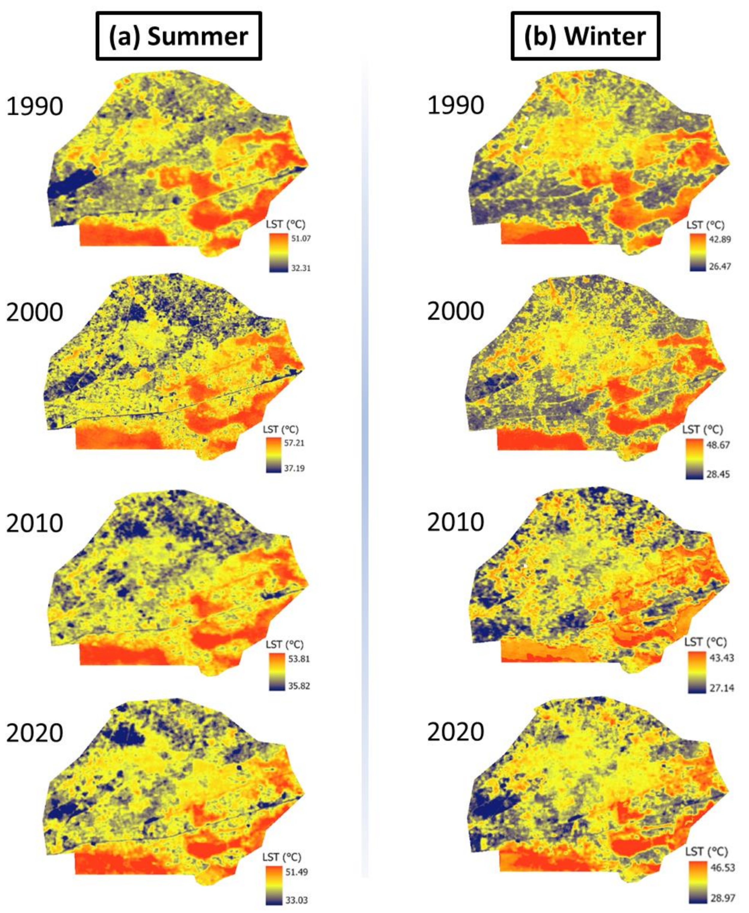Similarly, the city has gone through an industrialization process in the previous decades resulting in a 735% increase in industrial land use during 1974–2010 [65]. This urban growth and reduction in vegetation are the very reasons that the city has witnessed an increase in LST of both the summer and winter seasons (Figure 8), which is also reported for other urban areas around the world [4,16,66,67].

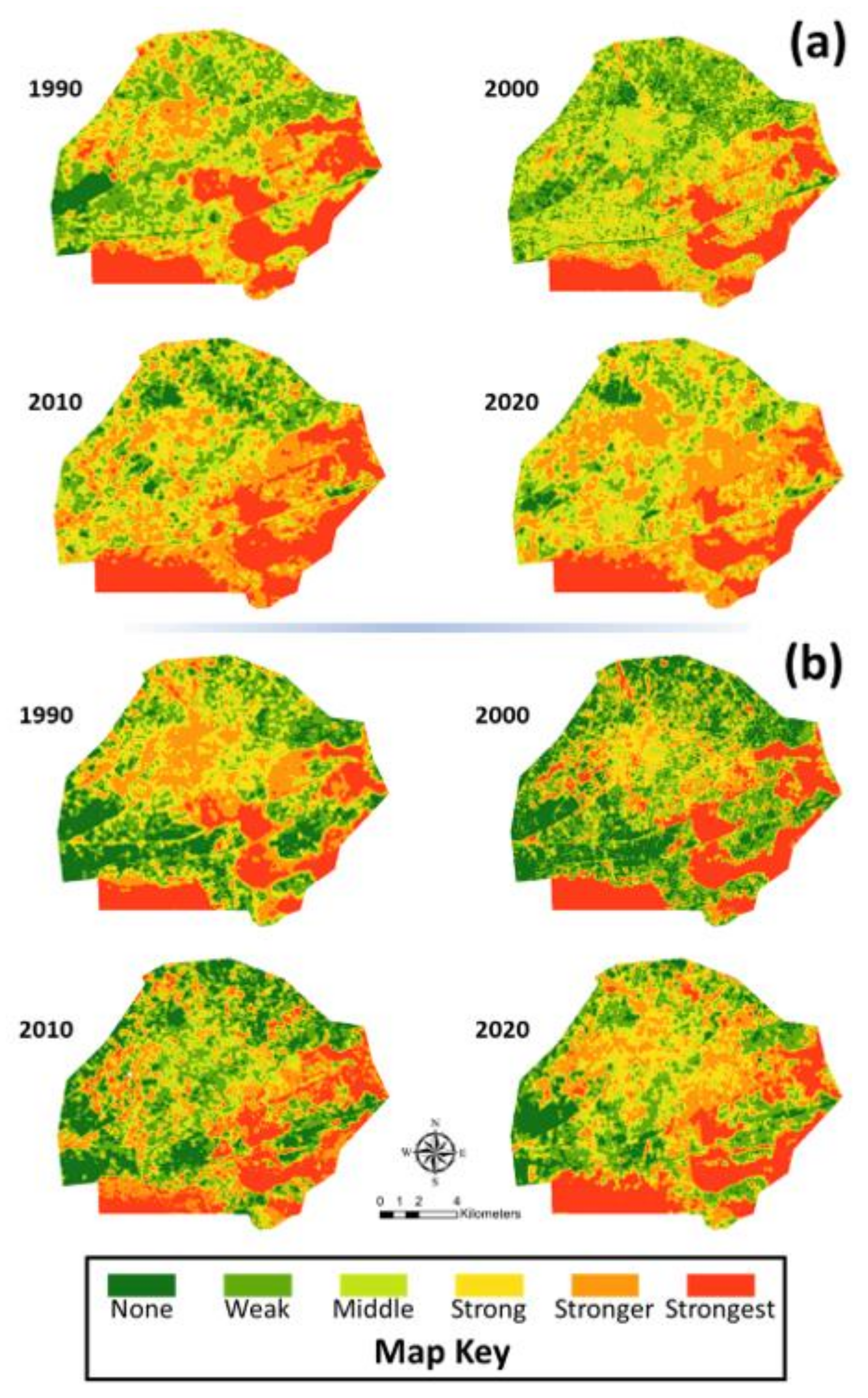
Urban heat island (UHI), the phenomenon describing the changes in urban climate due to human interventions, primarily affects UTFVI in cities. The transition of lower UTFVI zones into higher UTFVI strength regions (Figure 9, Table 13 and Table 14) is also a matter of concern for urban planners and designers as it would compromise the livability of the city without proper measures for both short- and long-term. It is well known that UTFVI adversely affects local air quality, wind patterns, and humidity resulting in reduced urban comfort and public health-related concerns [68]. On the other hand, the increments in built-up/impervious surfaces contribute towards stringer UHI effects in cities. Hence, the results on LULC changes, its spatial inconsistencies, and spatial-temporal UTFVI results from this study could progressively provide information on localized potential heat wave zones—assuring sustainable urban planning, design, and development via initiating essential action plans [16]. An unplanned increase/expansion in urban areas due to both strategic and economic influences resulting in the downdrift in natural systems such as vegetation as highlighted in this study, could potentially hamper the environmental health and sustainability of the city. Therefore, informed decisions and action plans such as urban green walls and other green infrastructure based on scientific evidence are integral to assure long-term sustainability [67].

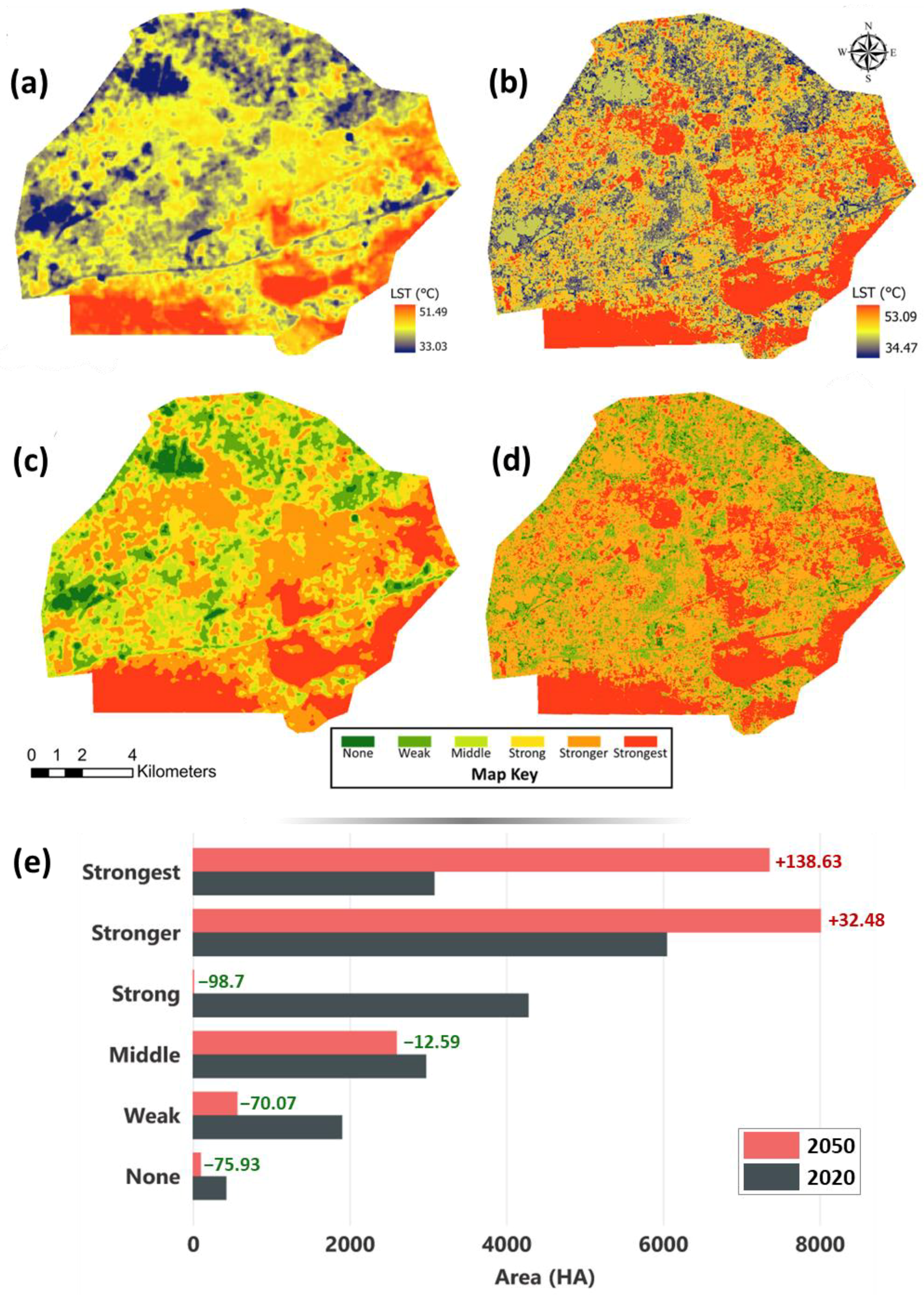
Increasing LST in the study area (Figure 8) as a result of thermal infrared waves produced by impervious surfaces and grey infrastructure (i.e., buildings) leads to UHI or UTFVI [16,69]. Another aspect resulting in a higher concentration of UTFVI in the southern part of the city is the presence of desert land. In the south of the city lies the Cholistan desert, which might be the primary reason behind the abrupt changes in the city’s microclimate [70]. However, further evaluation in this regard is recommended to understand the phenomenon from a micro-climate perspective. The situation of higher UTFVI can potentially impact urban societies through higher summer-time energy demands, emissions, air pollution, illness due to heat waves, and even deaths. To avoid these circumstances, strategies, and policies such as lower-emission technologies, the clean air act, no net vegetation loss, adoption of renewable energy resources, and implementation of nature-based urban designs can progressively help control the anthropogenic factors of UHI, resulting in more comfortable and livable urban places [71,72,73,74]. In this context, the results on variations in LST, UTFVI, and LULC across space and time provided in this study provide better insights into urban comfort by replacing the green with grey infrastructure/hardscape.

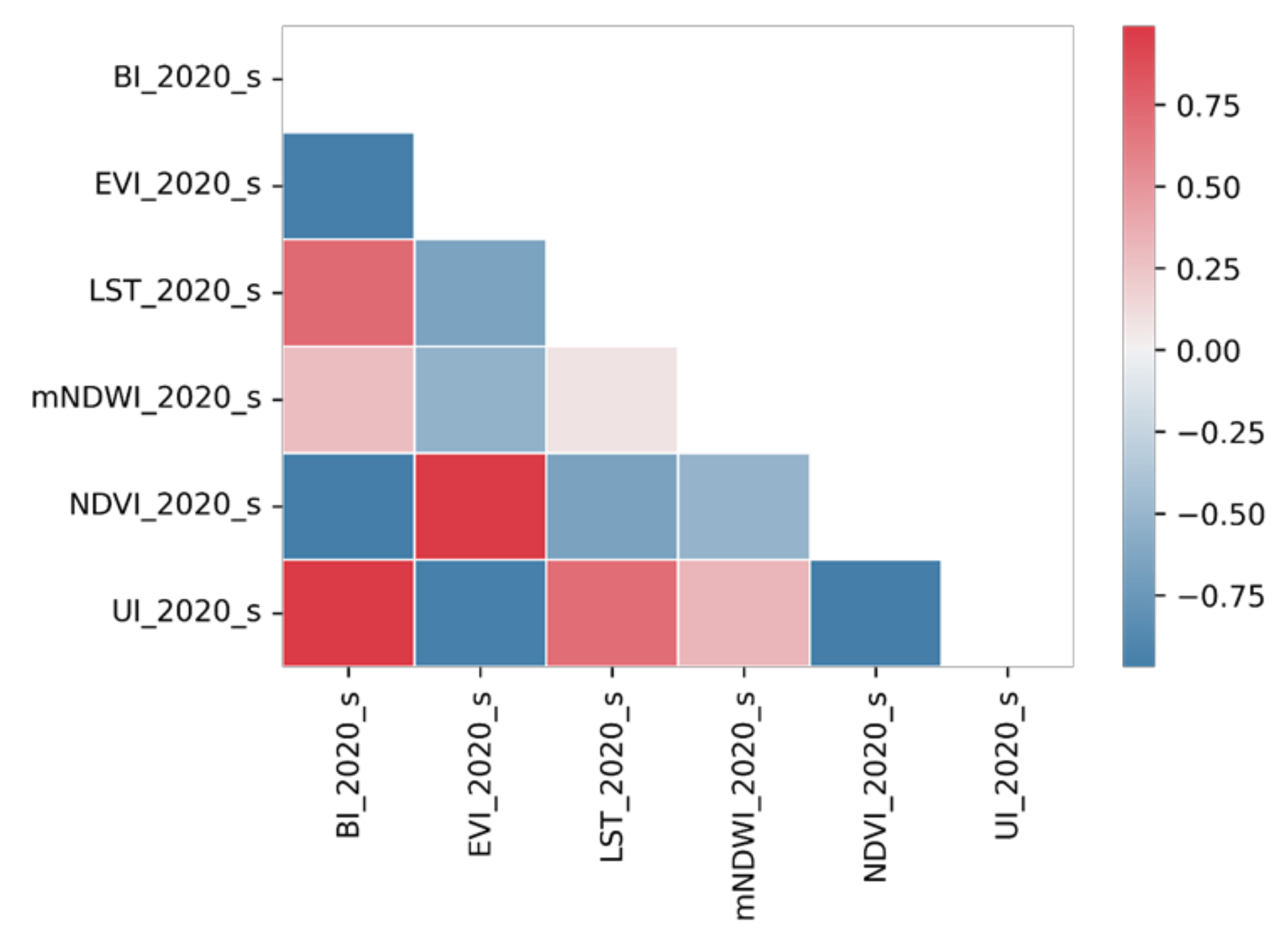
While this study relied on LULC and UHI, as indicators for urban thermal state, it is crucial to discuss some limitations, which may have indirectly influenced this study. In the evaluation of LULC, many aspects including the choice of model, training samples, spatial and spectral resolution of satellite image play crucial role. For instance, some studies [1,8,10] suggest that higher resolution images with machine learning approaches should be preferred which in most cases yield good accuracy. Another study [75] concludes that the sampling techniques play a great role in LULC classification. Similarly, for UHI evaluation, in situ temperature readings are required to ensure high accuracy of derived products [62]. This, require specialized instruments, with ability to work for longer periods. However, for historical assessment of meteorological events, satellite data with calibrated models are preferred [59,68]. To overcome such limitations, our study improvised with the following alternatives. First, since previous studies [1,10,23] support machine learning approach for LULC, we adopted this, which results in improved accuracy. Second, stratified sampling approach was used along with RF model, which minimize the need of extensive samples for training [75]. For UHI evaluation, as there was no historical high resolution numerical meteorological data available for Bahawalpur city, we adopted recent approaches from [17,59]. Through their approach, we first used satellite date for UHI historical assessment in the form of UTFVI. Later we used ANN models for future simulations of urban thermal condition through UTFVI.

The inclusion of the study area in the Special Economic Zones (SEZs) in Pakistan would upsurge industrial land use, which has already seen an increment of ~735% during 1974–2010 (https://pie.com.pk/bahawalpur-industrial-estate, accessed on 1 November 2022). This industrial development will further increase the population influx demanding more land resources for accommodation. LULC change prediction from this study can help design possible ways out with minimum trade-offs regarding vegetation loss in the future. Another potential strategy to tackle the UHI effect could be the adoption of “green ground” and “cool pavements” [76,77]. While the former is based on doubling the green and plant surfaces along with halving asphalt surfaces, the latter deals with increasing the albedo of horizontal grey land cover such as impervious surfaces. In the case of Padua, Italy, Noro and Lazzarin (2015) [76] showed that both strategies could reduce the daytime air temperature by 3 and 4 °C, respectively. Similarly, O’Malley et al. [39] show that UHI mitigation strategies such as the trees, shrubs, and grass (TGS), the use of high albedo materials (HAM), and urban inland water bodies (UIWB) have significant potential. However, in an urban environment, successfully implementing UHI mitigation measures also depends on building layout and form. Therefore, it is better if the provision of UHI mitigation measures is at the project’s conception stage. Hence, we strongly recommend further exploration of these mitigation measures (i.e., TGS, HAM, and UIWB) for the feasibility of their incorporation in the design of future urban development plans (i.e., expected LULC changes due to SEZ).

5. Conclusions

While LULC is an important indicator of sustainable urban development, evaluating the UHI effect provides a substantial gauge to measure the urban thermal state. Both of these indicators represent the sustainability and livability of rapidly urbanizing cities. In this context, the primary goal of this work is to provide spatial-temporal insights regarding LULC change, LST, and UTFVI during 1990–2020. For this purpose, the study leverages earth observation data from multiple satellite missions and spatial modelling approaches. Through literary review, this study overcome existing hurdles in geodata analytics by incorporating machine learning based RF model, which result in robust classification and by using ANN model with its proven results in meteorological forecasting. While a significant increase in urban areas (impervious surfaces) is observed during the past three decades, the CA-ANN-based prediction shows that a ~50% additional increase in built-up areas is expected by 2050 on the expanse of vegetation cover, primarily followed by barren land. During 1990–2020, since a decrease in vegetation and an upsurge in urban areas is observed, the LST has significantly increased. This situation directly influences the environmental conditions in the city along with having the potential to cause public health-related issues.

The transition of low UTFVI to strong and stronger zones during 1990–2020 also indicates reduced comfortability in the city—compromising livability in urban areas. The results are particularly helpful to city planners and relevant authorities in designing a sustainable environment via functional modifications and replacement of the current spatial distribution of LULC. Doing so would progressively enhance the livability of the city by mitigating the strong UTFVI effect. The effective LULC distribution and science-based smart utilization of land resources directly contribute to reducing the UHI effect, urban sustainability, and protection of natural systems within the cities—improving overall daily life. Lastly, for future studies, it is recommended to explore the possibilities of up-scaling the classification and prediction analysis of LULC and UHI up to regional and global scales with higher resolution. Furthermore, future studies are suggested to integrate big data analytics with open-source machine learning and deep learning modules (i.e., TensorFlow and Pytorch) and cloud computing platforms (i.e., Google Earth Engine) to find new possibilities in the context of sustainable cities, aiming to improve human thermal comfort.

References

1. Faisal, A.-A.; Kafy, A.-A.; Al Rakib, A.; Akter, K.S.; Jahir, D.M.A.; Sikdar, M.S.; Ashrafi, T.J.; Mallik, S.; Rahman, M.M. Assessing and predicting land use/land cover, land surface temperature and urban thermal field variance index using Landsat imagery for Dhaka Metropolitan area. Environ. Chall. 2021, 4, 100192. [Google Scholar] [CrossRef]
2. IPCC. The Physical Science Basis. In Contribution of Working Group I to the Sixth Assessment Report of the Intergovernmental Panel on Climate Change; Cambridge University Press: Cambridge, UK, 2021. [Google Scholar]
3. Szantoi, Z.; Geller, G.N.; Tsendbazar, N.-E.; See, L.; Griffiths, P.; Fritz, S.; Gong, P.; Herold, M.; Mora, B.; Obregón, A. Addressing the need for improved land cover map products for policy support. Environ. Sci. Policy 2020, 112, 28–35. [Google Scholar] [CrossRef] [PubMed]
4. Vinayak, B.; Lee, H.S.; Gedem, S. Prediction of land use and land cover changes in Mumbai City, India, using remote sensing data and a multilayer perceptron neural network-based markov chain model. Sustainability 2021, 13, 471. [Google Scholar] [CrossRef]
5. Twisa, S.; Buchroithner, M.F.J.L. Land-use and land-cover (LULC) change detection in Wami river basin, Tanzania. Land 2019, 8, 136. [Google Scholar] [CrossRef] [Green Version]
6. Nunez, S.; Verboom, J.; Alkemade, R. Assessing land-based mitigation implications for biodiversity. Environ. Sci. Policy 2020, 106, 68–76. [Google Scholar] [CrossRef]
7. Mejzini, I. The Phenomena of Urban Sprawl–Study Case of City of Prishtina; University for Business and Technology: Ferizaj, Kosovo, 2015. [Google Scholar]
8. Naim, M.N.H.; Kafy, A.-A. Assessment of urban thermal field variance index and defining the relationship between land cover and surface temperature in Chattogram city: A remote sensing and statistical approach. Environ. Chall. 2021, 4, 100107. [Google Scholar] [CrossRef]
9. Waleed, M.; Sajjad, M. Leveraging cloud-based computing and spatial modeling approaches for land surface temperature disparities in response to land cover change: Evidence from Pakistan. Remote Sens. Appl. Soc. Environ. 2022, 25, 100665. [Google Scholar] [CrossRef]
10. Kafy, A.-A.; Rahman, M.S.; Hasan, M.M.; Islam, M. Environment, Modelling future land use land cover changes and their impacts on land surface temperatures in Rajshahi, Bangladesh. Remote Sens. Appl. Soc. Environ. 2020, 18, 100314. [Google Scholar]
11. Koko, A.F.; Yue, W.; Abubakar, G.A.; Hamed, R.; Alabsi, A.A.N. Monitoring and Predicting Spatio-Temporal Land Use/Land Cover Changes in Zaria City, Nigeria, through an Integrated Cellular Automata and Markov Chain Model (CA-Markov). Sustainability 2020, 12, 10452. [Google Scholar] [CrossRef]
12. Liu, X.; Liang, X.; Li, X.; Xu, X.; Ou, J.; Chen, Y.; Li, S.; Wang, S.; Pei, F. A future land use simulation model (FLUS) for simulating multiple land use scenarios by coupling human and natural effects. Landsc. Urban Plan. 2017, 168, 94–116. [Google Scholar] [CrossRef]
13. Kaplan, G.; Avdan, U.; Avdan, Z.Y. Urban Heat Island Analysis Using the Landsat 8 Satellite Data: A Case Study in Skopje, Macedonia. Multidiscip. Digit. Publ. Inst. Proc. 2018, 2, 358. [Google Scholar]
14. Vargo, J.; Stone, B.; Habeeb, D.; Liu, P.; Russell, A. The social and spatial distribution of temperature-related health impacts from urban heat island reduction policies. Environ. Sci. Policy 2016, 66, 366–374. [Google Scholar] [CrossRef]
15. Mohajerani, A.; Bakaric, J.; Jeffrey-Bailey, T. The urban heat island effect, its causes, and mitigation, with reference to the thermal properties of asphalt concrete. J. Environ. Manag. 2017, 197, 522–538. [Google Scholar] [CrossRef] [PubMed]
16. Kafy, A.A.; Abdullah Al, F.; Rahman, M.S.; Islam, M.; Al Rakib, A.; Islam, M.A.; Khan, M.H.H.; Sikdar, M.S.; Sarker, M.H.S.; Mawa, J.; et al. Prediction of seasonal urban thermal field variance index using machine learning algorithms in Cumilla, Bangladesh. Sustain. Cities Soc. 2021, 64, 102542. [Google Scholar] [CrossRef]
17. Zhou, D.; Xiao, J.; Bonafoni, S.; Berger, C.; Deilami, K.; Zhou, Y.; Frolking, S.; Yao, R.; Qiao, Z.; Sobrino, J.A. Satellite Remote Sensing of Surface Urban Heat Islands: Progress, Challenges, and Perspectives. Remote Sens. 2019, 11, 48. [Google Scholar] [CrossRef] [Green Version]
18. Heaviside, C.; Macintyre, H.; Vardoulakis, S. The Urban Heat Island: Implications for Health in a Changing Environment. Curr. Environ. Health Rep. 2017, 4, 296–305. [Google Scholar] [CrossRef]
19. Tomlinson, C.J.; Chapman, L.; Thornes, J.E.; Baker, C.J. Including the urban heat island in spatial heat health risk assessment strategies: A case study for Birmingham, UK. Int. J. Health Geogr. 2011, 10, 42. [Google Scholar] [CrossRef] [Green Version]
20. Imran, M.; Mehmood, A. Analysis and mapping of present and future drivers of local urban climate using remote sensing: A case of Lahore, Pakistan. Arab. J. Geosci. 2020, 13, 1–14. [Google Scholar] [CrossRef]
21. Tariq, A.; Shu, H. CA-Markov Chain Analysis of Seasonal Land Surface Temperature and Land Use Land Cover Change Using Optical Multi-Temporal Satellite Data of Faisalabad, Pakistan. Remote Sens. 2020, 12, 3402. [Google Scholar] [CrossRef]
22. Saleem, M.S.; Ahmad, S.R.; Shafiq Ur, R.; Javed, M.A. Impact assessment of urban development patterns on land surface temperature by using remote sensing techniques: A case study of Lahore, Faisalabad and Multan district. Environ. Sci. Pollut. Res. Int. 2020, 27, 39865–39878. [Google Scholar] [CrossRef]
23. Dilawar, A.; Chen, B.; Trisurat, Y.; Tuankrua, V.; Arshad, A.; Hussain, Y.; Measho, S.; Guo, L.; Kayiranga, A.; Zhang, H. Spatiotemporal shifts in thermal climate in responses to urban cover changes: A-case analysis of major cities in Punjab, Pakistan. Geomat. Nat. Hazards Risk 2021, 12, 763–793. [Google Scholar] [CrossRef]
24. Hussain, S.; Mubeen, M.; Ahmad, A.; Akram, W.; Hammad, H.M.; Ali, M.; Masood, N.; Amin, A.; Farid, H.U.; Sultana, S.R. Using GIS tools to detect the land use/land cover changes during forty years in Lodhran district of Pakistan. Environ. Sci. Pollut. Res. 2020, 27, 39676–39692. [Google Scholar] [CrossRef] [PubMed]
25. Safder, Q.; Babar, U. Assessment of Urbanization and Urban Sprawl Analysis through Remote Sensing and GIS: A Case Study of Faisalabad, Punjab Pakistan. Int. J. Acad. Res. Bus. Soc. Sci. 2019, 9, 16–36. [Google Scholar] [CrossRef] [PubMed]
26. Shah, A.; Ali, K.; Nizami, S.M. Four decadal urban land degradation in Pakistan a case study of capital city islamabad during 1979–2019. Environ. Sustain. Indic. 2021, 10, 100108. [Google Scholar] [CrossRef]
27. Baqa, M.F.; Chen, F.; Lu, L.; Qureshi, S.; Tariq, A.; Wang, S.; Jing, L.; Hamza, S.; Li, Q. Monitoring and Modeling the Patterns and Trends of Urban Growth Using Urban Sprawl Matrix and CA-Markov Model: A Case Study of Karachi, Pakistan. Land 2021, 10, 700. [Google Scholar] [CrossRef]
28. Khan, A.A.; Arshad, S.; Mohsin, M. Population Growth and Its Impact on Urban Expansion: A Case Study of Bahawalpur, Pakistan. Univers. J. Geosci. 2014, 2, 229–241. [Google Scholar] [CrossRef]
29. Jat, M.K.; Garg, P.K.; Khare, D. Geoinformation, Monitoring and modelling of urban sprawl using remote sensing and GIS techniques. Int. J. Appl. Earth Obs. Geoinf. 2008, 10, 26–43. [Google Scholar]
30. Guan, X.; Liao, S.; Bai, J.; Wang, F.; Li, Z.; Wen, Q.; He, J.; Chen, T. Urban land-use classification by combining high-resolution optical and long-wave infrared images. Geo-Spat. Inf. Sci. 2017, 20, 299–308. [Google Scholar] [CrossRef] [Green Version]
31. Aarthi, A.D.; Gnanappazham, L. Urban growth prediction using neural network coupled agents-based Cellular Automata model for Sriperumbudur Taluk, Tamil Nadu, India. Egypt. J. Remote. Sens. Space Sci. 2018, 21, 353–362. [Google Scholar] [CrossRef]
32. Basit, M.; Sajjad, S.; Khan, M.I.; Ali, A.; Kurshid, S.K. Spatio-temporal trends of urban population in Pakistan. Asian J. Multidiscip. Stud. 2018, 6, 21–26. [Google Scholar]
33. Ahmed, T.; Shakeel, M.; Khalid, S.; Ali, A. Change of agricultural land use in residential land and its impact on the socio-economic status of the farmer in Bahawalpur City. Asian J. Soc. Sci. Humanit. 2015, 4, 3. [Google Scholar]
34. Kashif, M.; Awan, M.B.; Nawaz, S.; Amjad, M.; Talib, B.; Farooq, M.; Nizami, A.S.; Rehan, M. Untapped renewable energy potential of crop residues in Pakistan: Challenges and future directions. J. Environ. Manag. 2020, 256, 109924. [Google Scholar] [CrossRef] [PubMed]
35. Souza, C.M.; Shimbo, J.Z.; Rosa, M.R.; Parente, L.L.; Alencar, A.A.; Rudorff, B.F.; Hasenack, H.; Matsumoto, M.; Ferreira, L.G.; Souza-Filho, P.W. Reconstructing three decades of land use and land cover changes in brazilian biomes with landsat archive and earth engine. Remote Sens. 2020, 12, 2735. [Google Scholar] [CrossRef]
36. Yin, G.; Mariethoz, G.; Sun, Y.; McCabe, M.F. A comparison of gap-filling approaches for Landsat-7 satellite data. Int. J. Remote Sens. 2017, 38, 6653–6679. [Google Scholar] [CrossRef]
37. Imran, H.M.; Hossain, A.; Islam, A.K.M.S.; Rahman, A.; Bhuiyan, M.A.E.; Paul, S.; Alam, A. Impact of Land Cover Changes on Land Surface Temperature and Human Thermal Comfort in Dhaka City of Bangladesh. Earth Syst. Environ. 2021, 5, 667–693. [Google Scholar] [CrossRef]
38. Ghosh, A.; Sharma, R.; Joshi, P. Random forest classification of urban landscape using Landsat archive and ancillary data: Combining seasonal maps with decision level fusion. Appl. Geogr. 2014, 48, 31–41. [Google Scholar] [CrossRef]
39. Qian, Y.; Zhou, W.; Yan, J.; Li, W.; Han, L. Comparing Machine Learning Classifiers for Object-Based Land Cover Classification Using Very High Resolution Imagery. Remote Sens. 2015, 7, 153–168. [Google Scholar] [CrossRef]
40. Talukdar, S.; Singha, P.; Mahato, S.; Shahfahad; Pal, S.; Liou, Y.-A.; Rahman, A. Land-Use Land-Cover Classification by Machine Learning Classifiers for Satellite Observations—A Review. Remote Sens. 2020, 12, 1135. [Google Scholar] [CrossRef] [Green Version]
41. Vali, A.; Comai, S.; Matteucci, M. Deep Learning for Land Use and Land Cover Classification Based on Hyperspectral and Multispectral Earth Observation Data: A Review. Remote Sens. 2020, 12, 2495. [Google Scholar] [CrossRef]
42. Gilani, H.; Naz, H.I.; Arshad, M.; Nazim, K.; Akram, U.; Abrar, A.; Asif, M. Evaluating mangrove conservation and sustainability through spatiotemporal (1990–2020) mangrove cover change analysis in Pakistan. Estuar. Coast. Shelf Sci. 2021, 249, 107128. [Google Scholar] [CrossRef]
43. Vergni, L.; Todisco, F.; Di Lena, B. Evaluation of the similarity between drought indices by correlation analysis and Cohen’s Kappa test in a Mediterranean area. Nat. Hazards 2021, 108, 2187–2209. [Google Scholar] [CrossRef]
44. Wardhani, N.W.S.; Rochayani, M.Y.; Iriany, A.; Sulistyono, A.D.; Lestantyo, P. Cross-validation metrics for evaluating classification performance on imbalanced data. In Proceedings of the 2019 International Conference on Computer, Control, Informatics and Its Applications (ic3ina), Tangerang, Indonesia, 23–24 October 2019; pp. 14–18. [Google Scholar]
45. Werner, M. Shuttle radar topography mission (SRTM) mission overview. Frequenz 2001, 55, 75–79. [Google Scholar] [CrossRef]
46. Chen, Y.; Li, X.; Liu, X.; Huang, H.; Ma, S. Simulating urban growth boundaries using a patch-based cellular automaton with economic and ecological constraints. Int. J. Geogr. Inf. Sci. 2019, 33, 55–80. [Google Scholar] [CrossRef]
47. Liang, X.; Liu, X.; Li, D.; Zhao, H.; Chen, G. Urban growth simulation by incorporating planning policies into a CA-based future land-use simulation model. Int. J. Geogr. Inf. Sci. 2018, 32, 2294–2316. [Google Scholar] [CrossRef]
48. Saputra, M.H.; Lee, H.S. Prediction of land use and land cover changes for north sumatra, indonesia, using an artificial-neural-network-based cellular automaton. Sustainability 2019, 11, 3024. [Google Scholar] [CrossRef]
49. Datta, D.; Prasad, M.; Mandla, V.R. Study of various factors influence on land surface temperature in urban environment. J. Urban Environ. Eng. 2017, 11, 58–62. [Google Scholar] [CrossRef]
50. Tariq, A.; Riaz, I.; Ahmad, Z.; Yang, B.; Amin, M.; Kausar, R.; Andleeb, S.; Farooqi, M.A.; Rafiq, M. Land surface temperature relation with normalized satellite indices for the estimation of spatio-temporal trends in temperature among various land use land cover classes of an arid Potohar region using Landsat data. Environ. Earth Sci. 2020, 79, 1–15. [Google Scholar] [CrossRef]
51. Yang, F. Turbo decoder using local subsidiary maximum likelihood decoding in prior estimation of the extrinsic information. J. Electron. 2004, 21, 89–96. [Google Scholar] [CrossRef]
52. Mushore, T.D.; Mutanga, O.; Odindi, J.; Dube, T. Determining extreme heat vulnerability of Harare Metropolitan City using multispectral remote sensing and socio-economic data. J. Spat. Sci. 2018, 63, 173–191. [Google Scholar] [CrossRef]
53. Tucker, C.J. Red and photographic infrared linear combinations for monitoring vegetation. Remote sensing of Environment. Remote Sens. Environ. 1979, 8, 127–150. [Google Scholar] [CrossRef] [Green Version]
54. Xu, H. Modification of normalised difference water index (NDWI) to enhance open water features in remotely sensed imagery. Int. J. Remote Sens. 2006, 27, 3025–3033. [Google Scholar] [CrossRef]
55. Liu, H.Q.; Huete, A. A feedback based modification of the NDVI to minimize canopy background and atmospheric noise. IEEE Trans. Geosci. Remote Sens. 1995, 33, 457–465. [Google Scholar] [CrossRef]
56. Li, S.; Chen, X. A New Bare-Soil Index For Rapid Mapping Developing Areas Using Landsat 8 Data. ISPRS Ann. Photogramm. Remote Sens. Spat. Inf. Sci. 2014, 2, 139–144. [Google Scholar] [CrossRef] [Green Version]
57. Kawamura, M. Relation between social and environmental conditions in Colombo Sri Lanka and the urban index estimated by satellite remote sensing data. In Proceedings of the 51st Annual Conference of the Japan Society of Civil Engineers, Venue, Japan, 3–5 September 1996; pp. 190–191. [Google Scholar]
58. Ullah, S.; Ahmad, K.; Sajjad, R.U.; Abbasi, A.M.; Nazeer, A.; Tahir, A.A. Analysis and simulation of land cover changes and their impacts on land surface temperature in a lower Himalayan region. J. Environ. Manag. 2019, 245, 348–357. [Google Scholar] [CrossRef]
59. Dewan, A.; Kiselev, G.; Botje, D.; Mahmud, G.I.; Bhuian, M.H.; Hassan, Q.K. Surface urban heat island intensity in five major cities of Bangladesh: Patterns, drivers and trends. Sustain. Cities Soc. 2021, 71, 102926. [Google Scholar] [CrossRef]
60. Bahi, H.; Mastouri, H.; Radoine, H. Review of methods for retrieving urban heat islands. Mater. Today Proc. 2020, 27, 3004–3009. [Google Scholar] [CrossRef]
61. Guha, S.; Govil, H.; Dey, A.; Gill, N. Analytical study of land surface temperature with NDVI and NDBI using Landsat 8 OLI and TIRS data in Florence and Naples city, Italy. Eur. J. Remote Sens. 2018, 51, 667–678. [Google Scholar] [CrossRef] [Green Version]
62. Liu, L.; Zhang, Y. Urban Heat Island Analysis Using the Landsat TM Data and ASTER Data: A Case Study in Hong Kong. Remote Sens. 2011, 3, 1535–1552. [Google Scholar] [CrossRef] [Green Version]
63. Omar, N.; Sanusi, S.; Hussin, W.; Samat, N.; Mohammed, K.S. Markov-CA model using analytical hierarchy process and multiregression technique. In IOP Conference Series: Earth and Environmental Science; IOP Publishing: Bristol, UK, 2014; p. 012008. [Google Scholar]
64. Hamdy, O.; Zhao, S.; Osman, T.; Salheen, M.A.; Eid, Y.Y. Applying a hybrid model of Markov chain and logistic regression to identify future urban sprawl in Abouelreesh, Aswan: A case study. Geosciences 2016, 6, 43. [Google Scholar] [CrossRef] [Green Version]
65. Mohsin, M.; Minallah, M. Rapid Urban Growth and Change in Urban and Municipal Limits of Bahawalpur City, Pakistan: A Spatio-Periodical Discourse. J. Basic Appl. Sci. 2015, 11, 528–538. [Google Scholar] [CrossRef] [Green Version]
66. Shao, Z.; Sumari, N.S.; Portnov, A.; Ujoh, F.; Musakwa, W.; Mandela, P.J. Urban sprawl and its impact on sustainable urban development: A combination of remote sensing and social media data. Geo-Spat. Inf. Sci. 2021, 24, 241–255. [Google Scholar] [CrossRef]
67. Alavipanah, S.; Wegmann, M.; Qureshi, S.; Weng, Q.; Koellner, T. The Role of Vegetation in Mitigating Urban Land Surface Temperatures: A Case Study of Munich, Germany during the Warm Season. Sustainability 2015, 7, 4689–4706. [Google Scholar] [CrossRef] [Green Version]
68. Sejati, A.W.; Buchori, I.; Rudiarto, I. The spatio-temporal trends of urban growth and surface urban heat islands over two decades in the Semarang Metropolitan Region. Sustain. Cities Soc. 2019, 46, 101432. [Google Scholar] [CrossRef]
69. Wang, H.; Zhang, Y.; Tsou, J.Y.; Li, Y. Surface Urban Heat Island Analysis of Shanghai (China) Based on the Change of Land Use and Land Cover. Sustainability 2017, 9, 1538. [Google Scholar] [CrossRef] [Green Version]
70. Hassan, I.; Ghumman, A.; Aruba, W. Simulating precipitation of Bahawalpur and its adjoining Cholistan desert of Pakistandue to climate change. Int. J. Water Resour. Arid. Environ. 2019, 8, 109–117. [Google Scholar]
71. Kalnay, E.; Cai, M. Impact of urbanization and land-use change on climate. Nature 2003, 423, 528–531. [Google Scholar] [CrossRef] [PubMed]
72. Sajjad, M. Impacts, Drivers, and Future Adaptation Opportunities for a Warming Pakistan: Learnings from an Industrialized City. In Handbook of Climate Change Management: Research, Leadership, Transformation; Leal Filho, W., Luetz, J., Ayal, D., Eds.; Springer International Publishing: Cham, Switzerland, 2020; pp. 1–22. [Google Scholar]
73. Change, I.C. Mitigation of Climate Change. In Contribution of Working Group III to the Fifth Assessment Report of the Intergovernmental Panel on Climate Change; Regional Environmental Center: Ankara, Turkey, 2014; p. 1454. [Google Scholar]
74. Makido, Y.; Hellman, D.; Shandas, V. Nature-Based Designs to Mitigate Urban Heat: The Efficacy of Green Infrastructure Treatments in Portland, Oregon. Atmosphere 2019, 10, 282. [Google Scholar] [CrossRef] [Green Version]
75. Waleed, M.; Mubeen, M.; Ahmad, A.; Habib-ur-Rahman, M.; Amin, A.; Farid, H.U.; Hussain, S.; Ali, M.; Qaisrani, S.A.; Nasim, W.; et al. Evaluating the efficiency of coarser to finer resolution multispectral satellites in mapping paddy rice fields using GEE implementation. Sci. Rep. 2022, 12, 13210. [Google Scholar] [CrossRef]
76. Tubridy, F. Green climate change adaptation and the politics of designing ecological infrastructures. Geoforum 2020, 113, 133–145. [Google Scholar] [CrossRef]
77. Noro, M.; Lazzarin, R. Urban heat island in Padua, Italy: Simulation analysis and mitigation strategies. Urban Clim. 2015, 14, 187–196. [Google Scholar] [CrossRef]
Figure 1. Study area map. Please refer to the online version of the article to see the color image.
Sustainability 15 01416 g001
Figure 2. Schematic diagram of the workflow adopted in this study. Please refer to the online version of the article to see the color image.
Sustainability 15 01416 g002
Figure 3. Correlation between spectral indices (BI, EVI, mNDWI, NDVI, and UI) and LST for the 2020 summer. Please refer to the online version of the article to see the color image.
Sustainability 15 01416 g003
Figure 4. LULC classified maps of Bahawalpur for (a) 1990, (b) 2000, (c) 2010, and (d) 2020. Please refer to the online version of the article to see the color image.
Sustainability 15 01416 g004
Figure 5. Transitions of different LULC classes to urban (1990 to 2020): (a) spatial reference to transition, (b) estimated contribution of different LULC types to urban. Please refer to the online version of the article to see the color image.
Sustainability 15 01416 g005
Figure 6. (a) LULC for 2020 (simulated) and (b) predicted LULC for 2050. Please refer to the online version of the article to see the color image.
Sustainability 15 01416 g006
Figure 7. Urban sprawl trends from 1990 to 2050. Please refer to the online version of the article to see the color image.
Sustainability 15 01416 g007
Figure 8. Summer (a) and winter (b) LST changes and their spatial distribution across the study area between 1990–2020. The warmer colors (red shades) represent higher LST values, whereas the colder colours (blue shades) represent lower LST. Please refer to the online version of the article to see the color image.
Sustainability 15 01416 g008
Figure 9. Spatial-temporal distribution of UTFVI across the study area for (a) summer and (b) winter. The green shades represent no UTFVI, and the red shades represent the strongest UTFVI. The categories are defined based on the values of UTFVI as described in Section 2.6. Please refer to the online version of the article to see the color image.
Sustainability 15 01416 g009
Figure 10. (a) LST evaluated for 2020 (summer); (b) LST simulated for the year 2050 (summer); (c) UTFVI for 2020 (summer); (d) UTFVI simulated for 2050 (summer); (e) area change bar plot showing area changes between 2020 observed UTFVI and 2050 simulated UTFVI. Note that in (e), data labels in red shows increase (severity in UTFVI) while green shows area decrease (reduction in UTFVI). Please refer to the online version of the article to see the color image.
Sustainability 15 01416 g010
Figure 11. Spatial distribution of Std. Residual (a,c) and Local R2 using GWR model. The figure, (a,b) shows the results of GWR model-1 using Builtup-2050 and UTFVI-2050 whereas (c,d) shows GWR model-2 results using Vegetation-2050 and UTFVI-2050. Please refer to the online version of the article to see the color image.
Sustainability 15 01416 g011