1. Introduction
Several studies in the field of psychology suggest that emotional health is an important aspect of well-being. As a result, it is worrisome to observe that mental depression cases are on the rise across the world [
1]. A considerable portion of the population in many developed and developing countries suffers from mental illnesses [
2]. The emergence of the COVID-19 epidemic has made the situation worse [
3]. As a result, the ratio of mental patients to psychiatrists or psychologists has increased even more. According to one estimate, 62% of Americans experience acute stress in the months following COVID-19 recovery. Anxiety is one of the more long-term symptoms of post-COVID-19 syndrome (PCS), also known as Long COVID, a relatively new diagnosis. After recovering from the condition, between 23% and 26% of people, mainly females, experience mental health issues (including anxiety). Up to 25% of people, according to a 2021 study, experienced higher anxiety for at least 3 months after recovering from COVID-19. According to a 2021 study, if you have had COVID-19 [
3,
4,
5], you may have a greater risk of complications with major organ systems (kidneys, heart, lungs, and liver) after being discharged from the hospital. Furthermore, these patients are prone to cardiovascular disease (CVD). Human beings are emotional creatures, and this is a trait that sets them apart from other living beings [
6]. From relationships to decision-making, and even expressing oneself, emotions ultimately alter a person’s behavior [
7,
8]. A build-up of unprocessed emotions is a common trigger for anxiety or panic attacks [
9,
10,
11,
12]. These attacks exhibit physical symptoms that may easily lead to misdiagnosis. These symptoms include sharp chest pains, lightheadedness, nausea, difficulty breathing, dizziness, headaches, and even stomach aches. Internet of Things (IoT) devices, sensors, and artificial intelligence (AI) make users’ lives more comfortable and provide a feasible solution for healthcare applications [
13]. IoT devices such as sensors are embedded into physical devices along with machine learning methods to monitor and exchange data. In practice, there are faster ways through which doctors, with the help of IoT technology, can assess a patient’s emotional wellness. Global researchers from around the world have been working to develop automatic methods for tracking mental depression, particularly using EEG data. In this field, many machine learning and deep learning approaches, as well as various feature selection methods, are receiving greater attention.
Deep learning (DL) is one of the methodologies that can be used to calculate emotional factors. Several studies use DL-based classification algorithms to predict the user’s mental state from EEG signal data [
14]. The hardware measures the modes and frequencies of biological electro-signals gathered from brain waves. Electroencephalography (EEG) has been the most convenient brain imaging method that can reveal the brain’s electrical activity in real-time applications in daily areas of life. The brain dynamics when using an EEG are highly challenging to construe, especially if the signal comprises both noise and brain dynamics [
15]. Therefore, the need for signal filtration to achieve the desired electrical activity becomes important. The frequency domain of the EEG provides a view of the sequential events of processing streams in the brain. DL algorithms [
16,
17] offer a novel solution. Nowadays, researchers are using DL models for image or signal recognition and classification based on the Convolutional Neural Network (CNN), which is among the most successful algorithms.
Medical experts may be able to avoid some of these issues by using automated, accurate classification algorithms for EEG readings. The Depthwise Separable Convolution (DS-Conv) network presented here, which has a lower computational cost and fewer parameters than traditional heavy DL networks such as those in [
18,
19,
20], replaces them without sacrificing performance, having up to 27 times fewer operations and 32 times fewer parameters than VGG-16, but with only a 0.9 percent decrease in accuracy. In image-based recognition systems, a learning-based technique known as DS-Conv has recently been successfully employed for feature extraction [
16,
17,
18,
19,
20,
21]. The depthwise separable CNN (DSC) models outperform when compared with traditional manual feature extraction methods and some earlier transfer learning (TL) models. In this paper, the RCN-L anxiety and stress detection method being proposed is based on residual connections and a DS-Conv depthwise separable convolution neural network with a light gradient boosting machine (LightGBM). By combining residual connection and light gradient boosting machine (LightGBM) techniques, this paper presents a novel depth-separable convolution model called RCN-L. To develop an RCN-L system, the first step is to remove artifacts and convert the 1-D EEG data into a 2-D spectrogram image through a transformation phase. Later, the feature extraction step is performed on spectrogram images through the DS-Conv method and finally classified by the LightGBM classifier.
1.1. Aim of Study
The primary aim of this study was to detect emotions in undergraduate students who have recently experienced COVID-19 through analyzing their EEG signals. In this study, we used EEG signals due to several reasons. First, as a diagnostic measure, EEG is the preferred mechanism by which anxiety, stress, and normal emotions are detected by healthcare practitioners. Second, as pointed out in the literature review, there have been numerous studies detecting emotions from EEG with DL technologies with high predictive measures. However according to the best of our knowledge, we have not found any study, in the post-COVID-19 context, for measuring physiological disorder among undergraduate students. In addition, we compare non-COVID-19 and post-COVID-19 brain conditions of individuals to demonstrate the differences in detecting emotions using the proposed technique. As a result, the main EEG characteristics of each condition are identified, which can be potentially useful in making informed diagnosis decisions in clinical settings.
1.2. Major Contributions
The following are the important contributions of the presented method:
- (1)
Development of a novel RCN-L system to detect post-COVID-19 stress and anxiety symptoms among undergraduate students. The RCN-L model is less computationally expensive and requires fewer parameters.
- (2)
Preprocessing of the EEG signal to remove noise and convert it to a spectrogram image structure through the short-time Fourier transform (STFT).
- (3)
Efficient extraction of features from spectrogram images; a lightweight pre-trained CNN model which is based upon separable convolution has been developed for this purpose.
- (4)
Automatic classification of post-COVID-19 stress and anxiety by using a light gradient boosting machine (LightGBM), a machine learning technique.
- (5)
In terms of accuracy and the number of parameters, an efficient reduced-redundancy 2D separable convolution approach for diagnosis of post-COVID-19 stress and anxiety from EEG signals.
2. Literature Review
Several EEG-based state-of-the-art studies have been developed for the detection and classification of emotions using machine learning (ML) and DL algorithms. Since there is no single study on detecting the effect of post-COVID-19 on study or work performance, especially on employees’ or students’ mental health, many of the other state-of-the-art systems that have been developed are described in the following paragraphs.
According to the authors of the study [
22], EEG data was collected using four screen-printed active electrodes that were then integrated into a headband. The signal was then analyzed in real-time using an open-source software that extracts, classifies, and visualizes brain signals. In another study [
23], a database of standardized movie clips was created to target four types of emotions: surprise, sadness, disgust, and anger. The subjects were shown forty clips to use as elicitation material. For that study, fifty healthy people (25 men and 25 women) were considered. The study employed a deep learning network based on the long-term short-term memory (LSTM) model to distinguish negative and positive emotions.
In the paper [
24], the authors used 32 healthy volunteers who viewed a 40-min movie of emotional music, and their EEG signals were captured via 32 electrodes located on their skulls using the DEAP dataset. The three major components of feature extraction were asymmetric, regional, and temporal feature extractors. A convolution layer with 20 neurons was then utilized as the deep learning classifier, followed by a SoftMax layer. In another paper [
25], the authors collected a dataset while subjects were watching a 40-min video of music; 32 individuals had their EEG signals recorded. Following that, approximate entropy and the wavelet transform were utilized to extract EEG features. The support vector machine (SVM) and Random Forest (RF) machine learning classifiers were then used to recognize emotions. In the paper [
26], the authors used face features, EEG, and galvanic skin response (GSR) for multimodal emotion status. They used EEG signals because of their probability and reliability. To develop this system, they used Inceptionresnetv2 as the base network architecture. In another study [
27], the authors used EEG and peripheral physiological data to assess levels of valence, dominance, like/dislike, arousal, and familiarity in 32 participants while they watched 40 music videos for one minute each. The MobileNetV1 on the ImageNet dataset obtained an accuracy of 70.6% [
28], while the GoogleNet obtained an accuracy of 69.8%.
In another paper [
29], numerous studies were carried out using a variety of techniques, necessitating a thorough examination of the strategies employed for this work, as well as their feature sets and techniques. It serves as a guide for newcomers in designing an efficient emotion recognition system. The authors proposed emotion detection using electroencephalography (EEG) signals. The BiLSTM network learns spatial features and information from several brain regions and captures long-term reliance on the EEG signal. Moreover, the authors of study [
30] used a deep learning (DL) model to recognize emotions by utilizing the EEG signals.
In [
31], the models were combined with a variety of machine-learning approaches. These models were tested on two tasks: the first one was social anxiety disorder classification and emotion recognition, utilizing a dataset called DEAP for physiological signal emotion analysis. Five deep (CNN) convolutional neural network models were investigated to explore robust deep features [
32]. In [
33], the emergence of the COVID-19 epidemic had recently made the situation worse. The ratio of patients with mental depression to psychiatrists or psychologists was alarmingly low in many nations. The suitability of four neural network-based deep learning architectures that were developed to track mental depression from EEG data was investigated and compared in the study. In [
34], analyzing and classifying pre-recorded EEG data was also used to achieve a quantitative depression score. Furthermore, the results obtained by using raw EEG were far superior to those obtained using EEG. As discussed in many previous works, EEG has been studied only as a useful brain imaging tool, as discussed in [
35]. The key features used in previous work to determine the accuracy of EEG in emotion detection are different emotions. EGG signals are also applicable in emotion recognition since their devices are used in clinics to aid in the diagnosis of symptoms that are used as data for analysis for further medical interventions (
Table 1).
3. Materials and Methods
3.1. Data Acquisition
The EEG data were captured using the ThinkGear AM (TGAM) board and quantified in the frequency bands using the power delta (0.3–5 Hz), theta (4–11 Hz), alpha (12–16 Hz), and gamma (17–28 Hz). In the case study, an EEG signal data set (PostCovid-EEG) was used to verify the effectiveness of the suggested RCN-L methodology. There were extensive comparisons with existing EEG classification techniques. The Covid-EEG dataset contained different male and female subjects with different age groups. In fact, this dataset was collected based on the 30-min recording of EEG signals during the practice of five algebraic mathematical questions. This study engaged the participation of around 120 participants. The study’s participants were all undergraduate engineering students. With ages ranging from 20 to 26, there were 20 female students and 100 male students (20 with anxiety, 20 with stress, and 80 with normal states). The dataset was uneven, and this may have created bias issues. To handle this issue, this research employed 10-fold cross validation to remove the biases from the model. All participants were investigated for normal, stress, and anxiety emotions’ concerns after getting COVID-19. In general, the data was collected after a minimum of 30 days of COVID-19. These participants were already on medication and were under psychological treatment. They were selected at random, with the only condition being that they were in their first or second semester at university. All assessments were administered at the end of the semester to alleviate students’ anxiety about their academic responsibilities and/or exams.
It should be emphasized that the ThinkGear AM (TGAM) headset is a non-invasive brain–computer interface (BCI) device made for gathering unprocessed EEG data from the human brain for scientific study. The output signals have a frequency range of 0.2 Hz to 45 Hz, with a notch at 50 Hz for noise reduction caused by the AC power source. The subjects’ body movements, muscular movements, and eye blinking are kept to a minimum throughout the data collection. Artifacts such as visual, motion, sensory, and electrical artifacts can have a significant impact on the categorization method’s effectiveness. Therefore, it is crucial to introduce the artifact removal approach. Prior to being sent to the feature extraction phase, the EEG signals obtained from the sensors are first pre-processed to remove these artifacts. The denoising technique was used in this paper to divide the signals into sub-bands using the discrete wavelet transform (DWT).
3.2. Proposed Methodology
The primary goal of this paper was to confirm that emotion is impacted by post-COVID-19 scenarios. As indicated in the systematic diagram in
Figure 1, the proposed system combined residual connection and light gradient boosting machine (RCN-L) based on four primary phases. In the first phase, the multi-channel EEG signals are preprocessed to remove artifacts, and these 1-D EEG signals are converted into a 2-D spectrogram image. In the second phase, the depthwise and pointwise separable CNN (DSC-Conv) models with the residual network are utilized to extract relevant features. The unique DS-Conv-based classifier is then given these features, which creates probabilities for every output class in different time blocks. In the fourth phase, the LightGBM handling step integrates probabilities from several time blocks to boost detection confidence. To extract features from spectrogram images, the DSC and residual connection-based CNN models are used first. The images are then classified using LightGBM classifier into stress and anxiety. The next subsections will explain each of these phases in more detail.
3.2.1. Preprocessing and Signal Transformation
The EEG data were captured using the ThinkGear AM (TGAM) board and quantified in the frequency bands using the power delta (0.3–5 Hz), theta (4–11 Hz), alpha (12–16 Hz), and gamma (17–28 Hz). These multichannel EEG signals are recorded on human scalps, and they are invariably noisy (due to EEG artefacts and small interference). EEG signals are first subjected [
36] to a denoising technique to expose their features. A wavelet threshold denoising method was utilized in this paper as described in study [
36]. The Daubechies wavelet of order 6 (dB6) was selected as the mother wavelet for denoising using the discrete wavelet transform (DWT). Based on experiments, this paper selected dB6 over the entire Daubechies wavelet family to obtain the optimal wavelet. This work used a DWT noise removal method to remove eye blink or muscular distortions from EEG recordings. In de-noising physiological signals, wavelet de-noising outperforms signal frequency domain filtering because it preserves signal properties while reducing noise. Denoised EEG data can be used to analyze information from different emotional states, particularly stress and anxiety. After removing artifacts, the next step was to convert preprocessed 1-D multi-channel signals into 2-D spectrogram images by using the short-time Fourier transform (STFT) method.
The fast Fourier transform (FFT) is an algorithm that allows calculating the discrete Fourier transform, widely used in the process analysis of signals [
37]. The FFT estimates the magnitude and phase of the sinusoidal components’ periodicals, allowing one to reconstruct a signal as the linear combination of these components, which allows one to describe a signal in the frequency domain and in an analysis of time-dependent components. The fast Fourier transform (FFT) is a method to extract features and is used for extracting the finer emotional details such as spectral entropy and spectral centroid. The FFT extracts these simple features from the alpha, beta, and alpha to gamma frequencies. Given that theta and delta have extremely low frequencies, the lower frequencies are not needed for their lack of sufficient information in the FFT method. After the signal has been filtered and only the relevant signals are available, these signals are unidentified and need to be classified. The k-nearest neighbors (KNN) algorithm has a majority voting scheme, which is used to classify unidentified signals. The new data are given a classification with the highest number of votes. The majority vote schemes are used instead of similarity vote schemes because they are less sensitive to the outliers, which aids the FFT since it is a method for extracting the finer details [
20]. In fact, recent research has demonstrated that multiple fundamental frequency estimation performs exceptionally well in the magnitude spectrogram domain. As a result, we have applied spectrogram images to classify brain signals into stress, anxiety, and normal conditions.
The short-time Fourier transform (STFT) for non-stationary signals [
38,
39,
40,
41,
42,
43] is generally used (Equation (1)) even where a signal is divided into small segments and the smoothed FFT is calculated as a window for each segment, to avoid the effects generated by the truncations from the series; it is assumed that the signal has stationary features in short segments of time. When the frequencies vary wildly in the different parts of the program, no matter the size of the window, you could lose information. The inconvenience is that the analysis is made with a single resolution. In these cases, it is convenient to use Wavelets functions.
The parameters of Equation (1) are as follows:
x(n) is an input signal,
v(n) is the window size,
t0 is the window clearance,
f is frequency, and n is the number of current samples. Note that the window size effect is a small window (good time, bad time) and a big window (suitcase in time, good in frequency). According to Equation (1), the value of
t0 moves to the center of the window and the FFT is estimated for that segment that has a width the same as that of the window. This allows estimating the evolution of the spectrum by moving the window throughout the signal by adjusting the
t0 parameter. In addition, this process results in a three-dimensional graph that represents the energy of the frequency content of the signals and that varies over time. Finally, the energy of the signal can be estimated to elevate the STFT to the square (see Equation (2)).
where the spectrogram image is constructed and
x(n) is an input signal,
v(n) is the window size,
t0 is the window offset, the
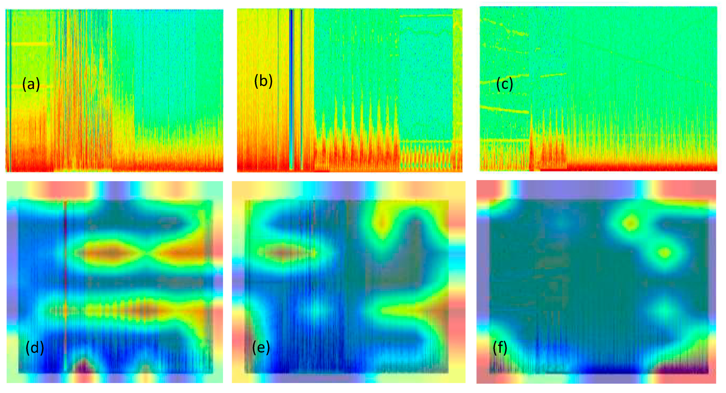
f parameter represents frequency, and n is the number of current samples. A visual example of signal preprocessing and transforming 1-D EEG signals into a 2-D image spectrogram is displayed in
Figure 2. Also, a spectrogram is a representation between three dimensions (temporal, frequency, and amplitude) of the energy distribution of a signal; an example of a spectrogram can be seen in
Figure 3.
3.2.2. Augmentation to Control Imbalance Data
The application of data augmentation techniques is carried out to control imbalance data. As a result, it is difficult to find a more appropriate and efficient augmentation method for designing the multi-label diagnosis system. Data augmentation operations often involve flipping, rotating, reflecting, shifting, zooming, contrasting, coloring, and noise disruption [
29,
30,
31].
To create the RCN-L model, all spectrogram pictures in the collected dataset were normalized from [0, 255 ] to [−1,1]. The CNN model requires a huge dataset to attain high-performance accuracy. Furthermore, due to an over-fitting issue, the CNN architecture’s performance deteriorated with a short dataset, implying that the model performs well on training data yet underperforms on test data. The data augmentation method was used in this research to enlarge the dataset to alleviate the problem of over-fitting. As a result, the dataset size can be enhanced using simple image processing methods as well as the data augmentation approach. The augmentation method is shown in
Table 2 and visually displayed in
Figure 4, including the parameters.
3.2.3. Features Extraction by RCN-L Classifier
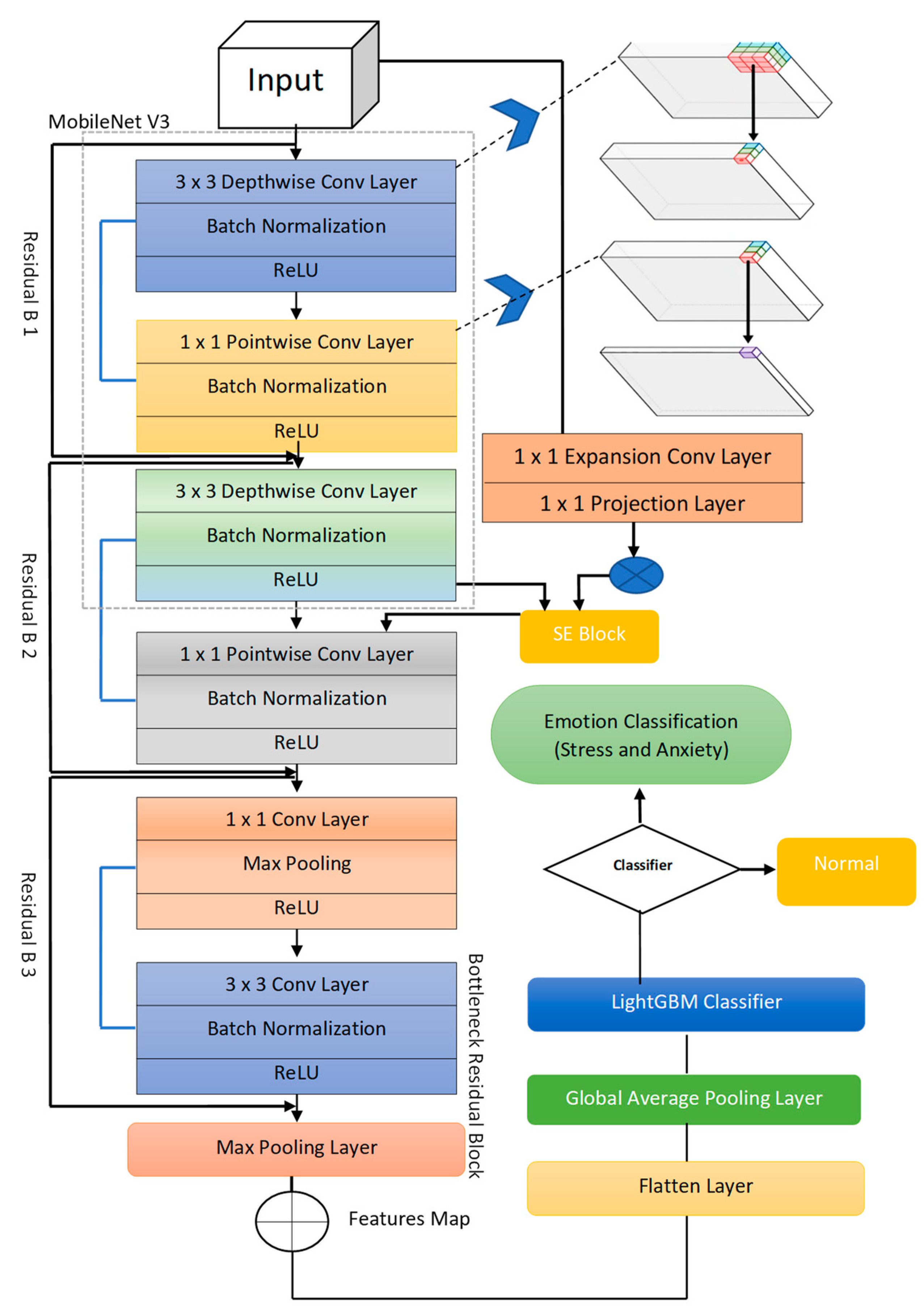
A newly proposed RCN-L system was provided to detect and classify human emotions into stress and anxiety with post-COVID-19 conditions. To develop this RCN-L system, two convolutional layers with a kernel size of (3 × 3), three residual blocks (b1, b2, b3) with two depthwise and pointwise convolutional layers and one pointwise convolution (PC1) layer, three Max Pooling layers (MP1, MP2, MP3), four batch normalization (BN) layers, and one convolution layer with a kernel size of 1 were used to build the feature map in this design. One projection convolution layer, one expansion layer, and one sequence and excitation block were also included in the network design. After that, one dense layer, one flat layer, one global averaging pooling layer, and finally, a LightGBM classifier with linear activation function, were used for classification. The systematic flow diagram is displayed in
Figure 5. In addition, Algorithm 1 displays all the steps used to develop an effective feature extraction strategy and those phases are explained in the subsequent paragraphs.
For depthwise convolutional layers, the kernel size was set to (3 × 3), with a boundary of 2 and a stride of 2. The pooling layers likewise employed a kernel size of (3 × 3) and a stride of 2. Batch normalization, which was applied right after each separable convolution layer before the activation function, may improve the efficiency and stability of deep neural network training. In addition, the Rectifier linear unit exponential linear units (RELU) function was used to define the output value of kernel weights and convolutional layers for each depthwise and pointwise convolutional layer. This adds a tiny amount of information to the classification process. Further, the flatten layer was used to flatten the feature, the dense layer was used to minimize the size of the feature, and the LightGBM classifier was used to classify the spectrogram image of the features into normal, stress, and anxiety.
EEG spectrogram signals are very complicated when there are EEG features to be extracted. As a result, the MobileNetV3 model was utilized as a backbone to extract and learn the most informative features from spectrogram images by using deep learning (DL) architecture. In practice, the MobileNetV3 block includes a fundamental building block called the residual block, which includes a depthwise separable convolution block and a squeeze-and-excitation (SE) block. The SE block is employed to pay more attention to the relevant features on each channel during training without sacrificing computational time. The MobileNetV3 was developed by Howard et al. in 2019.
MobileNetV3 is based on depthwise separable convolutions and was introduced for mobile and embedded vision applications in [
44]. MobileNet [
45] is a lightweight deep convolutional neural network class that is much smaller and runs much faster than many other popular models. Depthwise separate convolutions apply a single filter to each input to filter the data, then merge these filters together into a set of output features using 1 × 1 convolutions. These depthwise separable layers perform almost identically to traditional convolution layers but at a significantly faster pace and with a minor change. To implement minor change in the architecture, we have added a depthwise separable convolution, the normal convolution filters, and merge them into output features. This is divided into two layers, one for filtering and another for mixing. This reduces the size of the model and the amount of computing power required. Except for the final fully connected layer, which feeds into a softmax layer for classification with no nonlinearity, all layers are followed by batch norm and ReLU nonlinearity. Without counting depthwise and pointwise convolutions, MobileNet comprises different layers. The batch normalization layer and the rectified linear unit are added at the end of each convolutional layer. The MobileNetV3 has an inverted residual process for making linear bottlenecks with the increase in feature maps from 24 maps to 144 maps and the reduction in feature maps from 144 maps to 24 maps. Mobile Net’s architecture aids in depthwise separable convolutions, replacing computationally demanding convolutional layers, which are critical in computer vision applications [
46]. The depthwise separable CNN (DSC) offers two advantages for constructing a deep learning model: (1) it can help minimize parameters, and (2) it can be used to improve model generalization. As a result, it is safe to say that DSC improves detection accuracy and training effectiveness.
| Algorithm 1: Proposed depthwise and pointwise separable network |
Input: Input Tensor (), signals representation in form of spectogram.
Output: Extracted and generate feature map from preprocessed 2-D spectrogram image
Main Process:
Step 1. Depthwise and pointwise CNN blocks |
Step 2. Repeat for Each block
(a) Depthwise-CNN is applied to tensor x by kernel size of (3 × 3), which includes a number of filters, branch normalization, ReLU activation function is applied.
(b) Pointwise-CNN is applied to tensor x by kernel size of (1 × 1), which includes a number of filters, branch normalization, ReLU activation function is applied.
[End Step 2]
Step 3: Squeeze and Excitation (SE) block contains expansion (1 × 1), Projection (1 × 1) layers
Step 4. Model Construction
(a) (3 × 3) of two Conv layers, each with 32 and 64 filters, ReLU() function.
(b) Three skip-connections are applied to the network and each one skip includes two separable layers followed by maxpooling. The skip connection has Conv of with strides 2. |
| Step 5. Afterward, the feature map generated by using flatten layer. |
Depthwise separable CNN (DSC) was first introduced in the field of image classification by a few studies [
47]. DSC has been used in a variety of real-time applications in many studies. The conventional convolution is factorized into depthwise and pointwise convolutions via DSC. The single convolution filtering per channel is performed by depthwise convolution, which is followed by pointwise convolution, which is a linear combination of the depthwise convolutional output. The following is a formula for depthwise convolution:
The following is a formula for pointwise convolution:
DSC is an exceptional convolution class that combines pointwise convolution with depthwise convolution using a 1 × 1 kernel. When compared to regular convolution, DSC is specifically developed to reduce the computational complexity and learnable parameters. It was demonstrated that, when compared to the traditional convolution approach, 3 × 3 DSC might reduce the overall number of trainable parameters by eight to nine times. DSC achieves the same result by dividing the kernels into two and doing fewer multiplications. Each channel is considered separately, with one filter per channel being convolutional over that channel. Each input channel must be convolutional with a single precise kernel using the standard convolution method. By using a higher kernel size, you can reduce your processing costs even more. The DSC was developed as an alternative to the usual convolution structure in the present work to reduce the number of calculating operations while retaining CNN network generalization, as illustrated in
Figure 4. The DSC model divides the calculation of convolution into two stages: (1) for filtering, each channel is convoluted utilizing depthwise convolution; (2) for combining, pointwise convolution is convolutional kernel. A pointwise convolution is then used to connect the depthwise convolution outputs. A criterion convolution is used to make a new output set that filters out and merges the input in one step.
As demonstrated in
Figure 5, a deep neural network model was created by using MobileNetV3 as a backbone architecture. In general, the model used 1 × 1 convolution to minimize the dimension of the input spectrogram data cube, extracting a lot of spectral information. There are three residual units, R1, R2, and R3, which were then used to extract both spatial contextual and spectral aspects of the data cube indefinitely. Finally, instead of using the fully connected layer, a combination of 1 × 1 convolution and global average pooling (GAP) layer merged extracted abstract features and provided the most informative features for final signal classification task. Furthermore, this paper has presented per layer network architectural steps in
Figure 4. First, the network was fed with processed spectrogram data in the shape of 11 × 11 × 200 (200 being the number of bands). The first layer, C1, which has 38 of the 1 × 1 kernels, reconstructs channel properties from the raw input data while retaining spatial information. The R1 block, which consists of two 3 × 3 kernels with stride = 1, was then used to preserve spatial edge information. After the R1 block, the very first layer of R2 was a 3 × 3 filter with stride = 2 for down sampling, and the second layer was a 3 × 3 kernel with step size of 1 for generating 6 × 6 × 70 feature tensors.
The depthwise and pointwise separable CNN isolates channels by extracting only their input channels’ features rather than combining them to form new ones. Each channel requires a pointwise convolutional layer to improve channel correlation and recreate new input features. The architecture is made up of two depthwise and two pointwise convolutions that allow for substantially faster evaluation than classical convolution. For faster learning performance, a batch-normalization layer with the rectified linear unit (ReLU) activation function is used after the convolutional layer. Due to the rapid increase in training time and expense, large kernel sizes are no longer employed. Weights are regularly altered to choose the incoming data’s valid spatial information. ReLU was chosen as the activation function to introduce non-linearity into the network. Finally, every network produces a probability feature vector that forecasts the probability of each output class.
The loss function is used to calibrate the compatibility between both the desired output and network predictions. Weight matrices value reduction reduces network overfitting and facilitates model generalization due to the use of L2 regularization. The λ parameter shows the regularization parameter, and θ represents the set of filters, biases, and ReLU parameters to be estimated.
3.3. Transfer Learning
The goal of transfer learning (TL) [
32] is to provide a study area in DL to apply information gained, while addressing one issue to another that is comparable. Instance-based, parameterized, feature-representation, and relational knowledge transfer learning methods may be generally divided into four categories. The strategy that seeks to find effective feature representations that can be applied across domains, feature-representation transfer learning, is the most appropriate among these groups. In the suggested method, domain-independent image characteristics are extracted using pre-trained CNNs, which increases the transferability from source to target domain. The classification head is utilized instead of the top layers in a CNN that has already been trained on ImageNet. Pre-trained models are chosen wherever possible since the training time has been dramatically reduced. TL is primarily used to reduce training overhead. The pre-trained models combine feature extraction and fine-tuning to create new ones. We can adjust by adding additional layers to support the new classes. Here, we apply the fine-tuning approach. A pre-trained model is extended using the fine-tuning method to fit the requirements of the new dataset. The model does not need to be completely trained from the beginning. This shortens the training period. A few additional layers will be trained in this case by adjusting the weights while training. The weights will be adjusted during training to better match the characteristics of our dataset. The convolutional networks’ upper layers are often more specialized. The lowest layers pick up simple, universal properties that apply to many photos. The characteristics become more tailored to the dataset being used to train the model as they go up the network. Instead of replacing general learning, the primary objective of fine-tuning is to employ the specialized features with the required dataset. Fine-tuning can help to improve performance.
We demonstrated the suggested methodology using the MobileNetV3 network as a pretrained backbone architecture for effective features extraction. The initial weights were loaded into the basic models when they were created. The network was then trained using the fully connected model, which was added to this loaded model. The following sections go into great depth about each model’s specifics. To prevent overfitting, we simply made the last convolutional block more precise rather than the entire network. It makes sense to keep the first few blocks unchanged (more general features) and only fine-tune the last block since low-level convolutional blocks learn characteristics that are less abstract and more generic than those discovered from higher layers (more specialized features). To guarantee that the changes remain extremely small and do not influence the previously learned characteristics, fine-tuning is carried out at a very modest learning rate. The effectiveness of the network capacity decreases when more levels are frozen. As a result, we only learned the final classifier at the beginning, after freezing all the layers. Then, to have a better outcome, we thought about gradually unfreezing more layers, starting at the top. Networks that have been trained on a small amount of data may overfit the training set.
The weights utilized in the training of the original model were used as the beginning weights for the MobilenetV2 [
37] model. A dropout layer comes after the global average pooling layer. If overfitting is dealt with, increasing the network’s depth can enhance outcomes. Overfitting is avoided by using L2 regularization. The original model’s training weight from ImageNet was utilized to establish the weight. We utilized the binary cross-entropy logarithmic loss function because there are only two class variables.
3.4. Features Classification by LightGBM
The LightGBM classifier is used to recognize classes of emotions because of its efficiency in dealing with very small datasets, including its performance in high-dimensional domains, and this paper picked the LightGBM classifier for this investigation. They also have a three-class classification challenge, which is why they used LightGBM. LightGBM [
47,
48], and XgBoost have detection performance that is comparable to or greater than Random Forest. When the detection efficiency of LightGBM and XgBoost is compared, LightGBM training and testing times are much less than those of XgBoost. The Gradient Boosting Decision Tree (GBDT) algorithm has been improved with LightGBM. It merges the predictions of several decision trees to provide a final prediction that is highly generalizable. The overall steps for the LightGBM classifier are shown in Algorithm 2.
| Algorithm 2: Light Gradient Decision Boosting Machine (LightGBM) |
Input: Extracted Feature Data with labels y = 0,1 and Test Data
Output: Class Labels (Stress, Anxiety, Normal)
Process:
Step 1. First, initialize tree as a constant: for optimization and parameter defined for the classifier.
Step 2. Construct LightGBM tree by minimizing the lost function: |
| (6) |
- (a)
The LightGBM () classifier is perfectly trained on the feature samples that are extracted by separable CNN along with three residual blocks. - (b)
Get the next model in an additive manner:
| |
| (7) |
Step 3 Repeat Step 2 until the model reaches stop condition.
Step 4. Test samples are assigned the class label using the decision function of the below equation | |
| (8) |
The main concept of the LightGBM classifier is to combine numerous “weak” learners into a “strong” one. There are two main reasons why machine learning methods based on this concept should be designed. To begin with, “weak” learners are easily obtainable. Second, combining many learners often outperforms a single learner in terms of generalization. Several recent studies have shown that LightGBM outperforms other machine learning algorithms in a variety of tasks, including air quality prediction [
49] and tumor categorization [
50,
51]. For the most part, the features are mutually exclusive in a sparse feature space, so those features can securely bundle into a single feature. Therefore, the features create histograms from feature bundles in the same way that it is done from individual features. The complexity of histograms is therefore increased. This paper used it because the training time is greatly sped up without sacrificing accuracy. Another benefit of LightGBM is that it allows for the best possible division of category features. As a result, LightGBM may deal directly with data category attributes. On the other hand, many other machine learning methods do not support the category features processing and must first do the numerical translation (such as label encoding or one-hot encoding). This transformation converts the data into a format that machine learning algorithms can understand, but the data becomes sparse as a result. By using a grouping strategy, LightGBM allows for the best possible split of category features. This avoids the sparse data created by the numerical translation in this approach. The LightGBM typically has a lower number of decision trees and fewer leaves per decision tree in the final model. LightGBM saves time in the decision-making phase because of this model feature. The LightGBM is a tree-based technique that supports categorical features, making feature numerical translation and normalization unnecessary during the data preprocessing phase. In the decision-making step, the leaf-wise tree growth technique makes the matching efficient. Because of these benefits, we consider LightGBM to be very effective and have adopted it as the categorization system for stress, anxiety, and normal conditions following COVID-19.
5. Discussion
The fundamental purpose of this research was to develop a new deep-learning (DL) model for detecting and classifying stress and anxiety in undergraduate students who have been infected with COVID-19. The diagnosis of these emotions using EEG signals effectively achieved the complexity challenge, confined the dataset, and extracted the feature in the existing DL architecture quickly. Furthermore, when compared to state-of-the-art CNN-based classification approaches, it achieved better classification accuracy. As indicated in the systematic diagram in
Figure 1, the proposed RCN-L system has been developed based on four primary phases. In the first phase, the multi-channel EEG signals are preprocessed to remove artifacts, and these 1-D EEG signals are converted into a 2-D spectrogram image. In the second phase, the DS-Conv model with the residual network is utilized to extract relevant features. The unique DS-Conv-based classifier is then given these features, which creates probabilities for every output class in different time blocks. In the fourth phase, the LightGBM handling step integrates probabilities from several time blocks to boost detection confidence. To extract features from spectrogram images, the DSC and residual connection-based CNN models are used first. The images are then classified using LightGBM classifier into stress and anxiety. The advantages of the suggested (RCN-L) approach for identifying and classifying stress and anxiety emotions using preprocessed spectrogram images have been discussed. To detect stress and anxiety feelings, it was decided to utilize CNN as a foundation system based on DSC with a light gradient boosting machine (LightGBM).
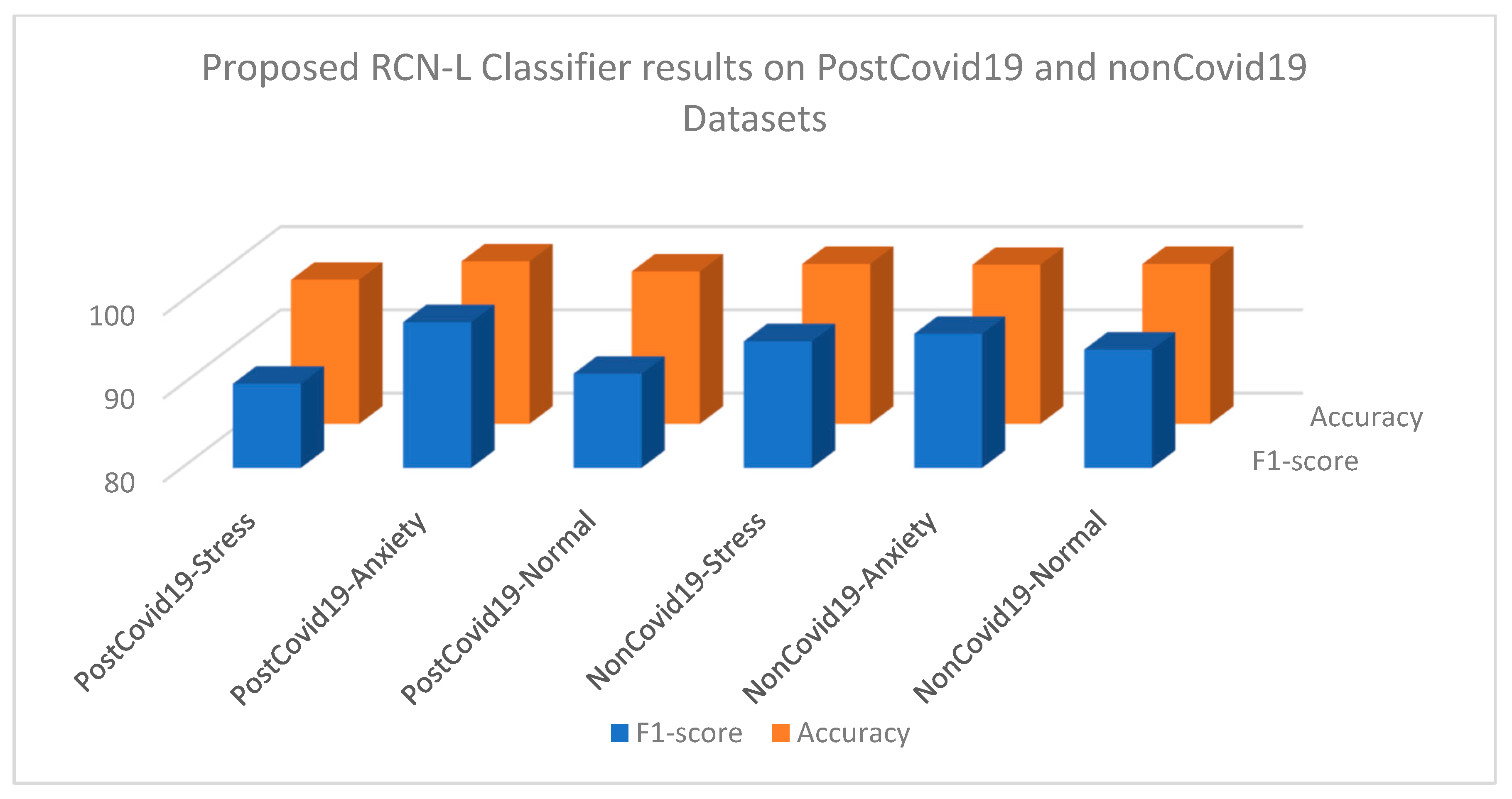
This paper collected datasets privately for the evaluation of the proposed work. First, it used the augmentation approach to enhance the data size. After that, this paper extracted features from spectrogram images using the first flow of the MobileNet model, which is based on depthwise–pointwise separable networks and residual connectivity. Finally, it used the feature map for the classification of the images into stress and anxiety spectrogram images using a LightGBM classifier. According to the results in
Table 4, the complete dataset delivered the best accuracy (91.98 percent) when utilizing the LightGBM classifier for identifying features to classify the stress, anxiety, and non-stress status tasks (almost perfect agreement). There was a need to use the confusion matrix to fully measure the detection performance. The confusion matrices revealed that the expected and actual labels were not in concordance. The genuine label for each row was presented on the row labels, while the predicted label for every column was displayed on the column labels. The color indicated the proportion of records in the same row as the total number of records. Consequently, depending on the test set classified by the RCN-L model, this study was able to acquire the results of two categories, such as anxiety and stress.
As shown in
Table 6,
Table 7,
Table 8,
Table 9,
Table 10,
Table 11,
Table 12 and
Table 13, the proposed approach RCN-L with LightGBM achieved excellent detection SE, SP, F1-score, and ACC. Using the proposed technique, the error rate on both datasets is extremely low. We were able to achieve 92 percent accuracy, precision, and recall using the DSC architecture and the LightGBM classifier. Similarly, the area under the curve (AUC) curve was also measured to show the performance of the proposed RCN-L model.
Figure 8 represents the various AUC curves when measured for different sets of epochs (50, 100, 150, 200, 250, 300, 350, 400). On average, the 0.92 AUC measures how well people recognize stress and anxiety emotions. In this paper, various segments of EEG spectrogram images were used to assess the model’s performance. The confusion matrix in
Figure 6 shows that the proposed model correctly detects all the emotion classes used in datasets. It was discovered that the projected label for every category does not become confused even when the model is trained on a limited dataset. Both categories are classified correctly. As can be seen from the confusion matrix, the suggested model RCN-L, along with a preprocessing stage to remove artifacts, has a greater detection accuracy.
It is preferable to conduct the EEG experiment on all participants at the same time of day to avoid the effects of time on cognitive ability and the implications of circadian rhythm for stress performance. The task nature and sample size had a direct impact on classifier accuracy, such as the limited duration of mental arithmetic tasks, which leads to low-performance accuracy [
43], and the mixed findings obtained with large numbers of participants in [
24,
42,
43]. It is worth emphasizing that most of the research has a small sample size, which means that the number of people participating was not large enough to overcome preconceptions based on individual variations. Furthermore, in these experiments, the data augmentation technique was applied to increase the dataset size. Many studies have provoked stress in controlled situations, whereas developing a technique that can withstand real-world scenarios, such as virtual reality, is a superior method. Furthermore, the ground truth that is required to train the classifier by separating people into stress and anxiety groups is a significant aspect that determines stress assessment findings. Most of the research used a mathematical questionnaire, a psychological interview, or both, to determine this labeling. However, because of the heavy reliance on participants, these two methodologies were unable to provide a direct assessment of the presence of mental stress. Unlike in simulated tests, labeling subjects in real-world tasks is a considerable problem. This study is proposing EEG feature extraction techniques for increasing stress detection, such as phase synchronization and source localization, as future research.
Despite having a small dataset from our study and experiments, the post-COVID-19 EEG images were significantly different from the others in all statistical tests. There are several techniques for extracting features, including time series domain and frequency domain techniques, and new techniques are always being created. For ML or DL to conduct dimensional reduction and improve prediction accuracy, meaningful feature extraction is essential [
46]. The current study employed coherence approach to extract robust features in case of noise from 2-D spectrogram images. Our findings can be used to provide diagnostic data and support tailored treatment decisions. The EEG using DL has shown encouraging results for predicting treatment responses. Additionally, compared to the paradigm involving experimental stimulation, the task-free and resting-state technique for EEG recording requires less measuring time, making it more accessible and scalable.
As a result, we discovered that, depending on the diagnosis, a DL technique employing EEG may accurately predict major mental diseases to varying degrees. Several EEG feature characteristics were illustrated in each condition categorization model. EEG-DL is a promising method for categorizing psychiatric diseases. It has the ability to support clinical judgments based on evidence and offer objectively quantifiable biomarkers. Future medical healthcare that uses BCI and automated diagnostic technologies might be useful.
The mental healthcare field is evolving quickly due to data and computational science breakthroughs. The range of data we can measure has increased with regard to neurological processes and objective indicators. Furthermore, the application of machine learning (ML), deep learning (DL), or artificial intelligence (AI), has grown. Out-of-sample estimates allow machine learning (ML) to prospectively evaluate the efficacy of predictions on new data (test data) that was not used for model fitting (training data), thereby producing results that may have a high level of clinical translation. This method differs from traditional inference based on null hypothesis tests (such as the t-test and analysis of variance), which retroactively concentrate on in-sample estimates and group differences and lack individualized explanation. ML is expected to supplement or even replace clinical judgments, such as diagnosis, prognosis, and treatment outcome prognosis.
The current study contains a few drawbacks. First, there was no control over the noise or muscular movements on the selected EEG signals. Second, diagnoses were made close to the time that EEGs were taken, so we cannot completely rule out the possibility of individuals having mixed findings who were later diagnosed with various diseases. Third, the sample comes from a single center and only in a certain environment. The model should be evaluated for different environments in terms of race and nationality. Finally, we did not prospectively validate the model because our methodology is retrospective. Moreover, no additional samples were received for external validation. As a result, more samples must be used to confirm the results before making any generalizations.
The experimental results show that classification accuracy for emotions is possible because we developed a lightweight pre-trained model with a computational efficiency solution which requires fewer parameters. When compared to other classifiers, our proposed RCN-L system outperforms them, which proves that the proposed model is unique compared to the state-of-the-art approaches.
6. Conclusions
Sensors embedded in physical devices, as well as machine learning methods, are used by IoT devices to monitor and exchange data. As the number of cases of post-COVID-19 rises rapidly, it is more important than ever to detect, diagnose, and control emotions early. In this study, the RCN-L model with preprocessing steps has been proposed as a stress-inducing protocol, and different aspects of EEG multichannel signals have been examined using time-series physiological data collected from 120 undergraduate students. EEG-based deep learning approaches to emotion detection are computationally demanding, limiting memory potency, training, and hyperparameter tuning. As a result, they are inappropriate for real-time applications with limited computational resources, such as the detection of post-COVID-19 anxiety and stress. The accuracy, precision, recall, F1-score, and AUC of the suggested redundancy-reduced depthwise separable convolution network were 0.9163, 0.9246, 0.9282, 0.9264, and 0.9263, respectively. There were only 20,686 parameters employed in the proposed approach. The proposed network avoided the time-consuming detection and classification of emotions for post-COVID-19 while still achieving impressive network training performance and a significant reduction in learnable parameters. With the use of electroencephalography, we sought to create a machine-learning (ML) classifier that can identify and contrast the main mental diseases (EEG). In the past, we gathered information from medical records. Models for the categorization of individuals with each disease were established using a combination of factors at different frequency bands. This paper also concluded that emotions are impacted by post-COVID-19 scenarios. In the future, we will use this RCN-L model for post-COVID-19 patients to analyze employee performance.


