Article

Relationship among Plant Functional Groups, Soil, and Moisture as Basis for Wetland Conservation

by
Fevziye Aslan
1,
Ricardo Mata-González
1,
David Eduardo Prado-Tarango
1,*,
Matthew Hovland
1,
Jenessa Stemke
2 and
Carlos G. Ochoa
1
1
Department of Animal and Rangeland Sciences, Oregon State University, Corvallis, OR 97331, USA
2
College of Forestry, Oregon State University, Corvallis, OR 97331, USA
*
Author to whom correspondence should be addressed.
Sustainability 2023, 15(19), 14377; https://doi.org/10.3390/su151914377
Submission received: 28 July 2023 / Revised: 25 September 2023 / Accepted: 27 September 2023 / Published: 29 September 2023

Abstract

:
This study characterized the relationship between plant species, soil, and moisture dynamics in the Willamette Valley (Oregon, USA) to obtain a base framework for wetland conservation and restoration. We identified 24 dominant plant species, including the exotic invasive Dipsacus fullonum, distributed throughout the wetland. Plant community analysis indicated that (1) soil moisture during the dry season (August to October) and (2) soil bulk density were the major abiotic drivers of plant community structure. Water potential measurements confirmed the community analysis. Juncus (rush) species appeared to be more tolerant to drought than other typical wetland species. Therefore, dryer conditions due to climate change or water diversion may favor rushes’ persistence. We also found that the dominance of D. fullonum may also negatively affect the native plant species’ survival, which highlights the need for proper management practices. To prevent further vegetation deterioration in sensitive wetland areas, we recommend avoiding hydric diversions to maintain the water supply, exploring manners of controlling invasive species, and preventing livestock grazing. The results of this study contribute to foundational and practical knowledge concerning the influence of soil conditions and moisture availability on the physiological response and distribution of wetland plant species that is required for conservation and management.

1. Introduction

Despite their high environmental importance, 50% of the wetlands around the world have disappeared in the last 100 years [1]. In the Willamette Valley (OR, USA), wetlands have been exposed to extensive land conversion since the 19th century because this area has fertile soil and abundant rainfall, which are significant factors for agricultural practices [2]. Before the introduction of developed agriculture, the Willamette Valley provided a broad composition of wetland habitats supporting a high diversity of native plants and animal species [3]. A recent survey demonstrates that despite the implementation of wetland conservation laws since the 1960s, wetlands continue experiencing substantial annual losses, alteration, and conversion [3]. In addition to the traditional threats posed by agricultural conversion, climate change represents a global novel threat for wetlands around the world [4].
Wetland alteration and conversion have negative influences on ecosystem goods and services [5]. Wetland conservation practices should be focused on the recovery of functions and processes and some basic practices include fencing and grazing exclusion [6]. However, those practices only target current disturbances and do not consider the effects of historic land use, which brings more challenges for conservation such as the possible presence of invasive species, soil erosion, and sedimentation [6]. Identifying the composition of plant communities at the local level and understanding their relationship to the ecosystem’s abiotic factors (such as soil physical characteristics and moisture dynamics) is essential for wetland conservation and restoration [7]. Some important soil physical properties such as moisture content, texture, and bulk density directly affect hydraulic conductivity, water storage, water availability, and vegetation structure [8]. The water regime primarily determines the wetland plant community composition, and there is a strong correlation between vegetation and various water regimes within a single wetland, which determines spatial and temporal heterogeneity in wetland vegetation [9].
It is generally accepted that wetland plants tend to be highly sensitive to hydrological variations [7]. Yet, within a wetland plant community, a gradient in topography means some plant species must tolerate constant flooding while other species must withstand drought when the water table drops beyond their root system’s reach [10]. Topographical and micro-topographical variations contribute to differences in water movement at a wide range of spatial scales in wetland areas [11]. This variability makes it difficult to predict the effects of different water regimes on the composition, abundance, and distribution of wetland vegetation [12]. Although water regime is an important factor controlling the composition of vegetation in wetlands and other types of land, invasion by weeds and undesirable species may be influenced by the history of degradation of an area.
The protection and conservation of wetlands require assessment and monitoring at the local level [4]. Global assessments of wetlands provide general portraits of their status, but they are only as precise as the available data [13]. Here, we collected data in a local wetland and applied geospatial and multivariate data analyses to achieve the following objectives: (1) to assess the present plant communities; (2) to understand the relationship between plant functional groups, soil characteristics, and moisture; and (3) to evaluate important plant species’ water stress responses to drought. As a basis for the conservation of wetlands, we are trying to answer the question: how do the changes in soil properties and soil moisture influence the plant functional groups within a wetland?

2. Materials and Methods

2.1. Study Site

This study was conducted from 30 July 2018 to 15 April 2020 at a conservation wetland at the Oregon State University Sheep Farm in the Willamette Valley, OR, USA (approximate longitude 123.33145° W, latitude 44.591987° N, and elevation 123 m above sea level). We selected the study period because we wanted to have a better understanding of the plant communities during the whole year in the wetland. Our research site comprised an area of about 2.1 ha and was located near the streamside at Oak Creek. There is a canal in the wetland that drains into Oak Creek during the wet season. Inside the study area, six transects were systematically established to represent the whole study area, to monitor soil water content, and to evaluate the composition of the vegetation. These transects were approximately 30 m apart from each other and were 60 m in length. For a relatively small study area like ours, systematic sampling can be as or more adequate to represent a community than random sampling [14,15].
The wetland, which is part of a Conservation Reserve Enhancement Program, has been fenced since 2010 to enhance habitat and protect water resources. Before that, management of the area included grazing as the main type of disturbance and some areas were periodically mowed. Furthermore, some areas of the wetland were planted with ash trees (Fraxinus spp.) and willow (Salix spp.). These trees were planted in a nonhomogeneous manner in some parts of the area and represent a minor component of the vegetation. Thus, these trees were not considered as part of this study. We were interested in a better understanding of the vegetation and their interactions with soil and water resources of this wetland to devise a more specific management/conservation plan that restores wildlife habitats and enhances water quality.
The soil of the area is a Bashaw clay with 3% to 12% slope, poorly drained with very fine pores on flood plains [16]. Soil texture in the study area is characterized as clay loam, sandy clay loam, sandy loam, clay, and loam. Saturated soil in the vicinity of channels supports mostly hydrophytic vegetation. The climate in the study area is mild, with cool, wet winters and hot, dry summers. The daily average air temperatures during the study years of 2018–2019 ranged from about −0.7 °C in February to around 30.8 °C in August. Long-term mean annual air temperature in the study area is approximately 11.6 °C. The study site receives about 1085 mm of precipitation annually, most of which comes as rain during the winter. Approximately 75% of the precipitation in the area occurs between October and March.

2.2. Plant Species Composition

The line-point intercept method was used to determine vegetation cover (basal cover) along the six transects of the study area in May 2019. A 60 m tape measure was placed on each transect to read vegetation cover and soil surface cover every 0.5 m [17]. At each site, plant functional groups were classified based on growth form: rushes, sedges, grasses, or forbs. We used this classification from a functional/management perspective; the area has been historically managed for livestock grazing, so separating the palatable grasses from other groups was important. Sedges can also be palatable for livestock, but rushes are not. The forbs of our study area are also not palatable, including Typha latifolia. Data from each 60 m transect were used to calculate average total cover by plant species and relative cover of each plant type group.

2.3. Soil Sampling

We collected soil samples for soil texture and soil cores for soil bulk density. Topsoil cores were collected in September 2018 to determine soil texture and bulk density. One soil core was collected every 5 m (starting from 0 m) on the six 60 m transects (13 samples for each transect), for a total of 78 samples using a soil core sampler (5 cm diameter × 7.5 cm length). Soil texture (clay, silt, and sand content) was estimated using the hydrometer method [18]. Prior to soil texture analysis, 50 g of dry soil was treated with 5 mL of 30% H2O2 to oxidize any organic matter. We added 50 mL of 10% Sodium hexametaphosphate (NaHMP) and placed the suspension on a shaker overnight to disperse soil aggregates. Then, the soil suspension was transferred to a 1 L graduated cylinder and measured with a hydrometer at multiple time points to determine the specific gravity of the suspension [19]. Soil cores were weighed, oven-dried at 105 °C for 24 h, then reweighed to determine soil volume and dry soil weight. Dry soil bulk density was calculated by dividing the dry weight of soil (g) by the soil volume (cm3). Soil bulk density was obtained once in May 2019.
We also collected soil volumetric water content (20 cm depth) every five meters along each transect using a HS2P HydroSense II (Campbell Scientific, Logan, UT, USA) portable soil water probe. Similar to the measurements of soil texture and bulk density, 13 measurements of soil volumetric water content were obtained on each transect. To determine temporal changes in soil volumetric water content, we collected data weekly from March 2019 to March 2020.

2.4. Water Potential Sampling

Plant water potential (Ψ) was determined to estimate the physiological stress response of four representative plant species to changes in soil volumetric water content. Stem water potential of Juncus patens and Juncus effusus and leaf water potential of Typha latifolia and Scirpus microcarpus were measured for 3 days at the end of July, August, and September 2019 (the driest period of the year). These measurements were collected during midday (Ψm; 12:00–14:00 pm) and predawn (Ψpd; 03:00–5:00 am) using a Scholander-type pressure chamber (PMS Instruments, Albany, OR, USA). Vegetative stems or leaves (n = 3) were sampled using scissors, then clipped samples were measured in a short time at the same midday and predawn periods. We evaluated water potential in only four representative species from the 27 plant species that were found in the study area because of time constraints and because those four species were the main ones available during the dry period of the year. Some other plant species, such as Alopecurus pratensis, were not accessible during late summer because they typically die back during the dry period and regrow during the spring, the wet period. In order to understand the responses of J. patens, J. effusus, T. latifolia, and S. microcarpus to water stress, we also measured soil volumetric water content at the base of the plants that were evaluated for Ψ on the same day.

2.5. Geospatial Analyses

The collected data (soil bulk density, soil texture, soil moisture) were geo-located using a Juniper Systems Geode GNS2 Sub-meter GPS Receiver (Juniper Systems, Logan, UT, USA) in the 6 linear transects. The accuracy of the Geode with SBAS (WAAS) correction is <60 cm 2DRMS. Spatial analysis was conducted using the Spatial Analyst Extension in ArcMap 10.8 (ESRI, Redlands, CA, USA). Clay content and bulk density were analyzed once, as these properties are relatively static. Interpolation was used to display spatial variation in each property across the sample site, and the spline function was the specific interpolation tool used with default Environment Settings, cell size of 0.31 m, and smoothing factor of 0. A hillshade created from LiDAR data with a spatial resolution of 1 m was used as a backdrop and displayed using the cubic convolution display setting (for continuous data). LiDAR data were acquired from State of Oregon Department of Geology and Mineral Industries (DOGAMI).
The soil water content measurements that were taken through the year of study across the study area were used to model water content surfaces across spatial and temporal scales using GIS. Although soil moisture measurements were performed weekly throughout the year, we chose to model soil moisture to exemplify variations at two times: during the wettest month (April) and the driest month (August). Volumetric water content maps were displayed using the same color scheme (10% increments) across all dates to allow for comparison across time. Intuitive colors were used for their respective maps. For ease of interpretation, defined class sizes were used for all legends and class breaks, such as increments of 0.2 g/cm3 for bulk density size class range. Contour lines were added for added visual distinction between classes.

2.6. Statistical Analysis

Plant community analysis was conducted using plant occurrence data, with plant species grouped by functional groups based on growth form (rushes, forbs, grasses, and sedges), as well as one group for litter, and one for bare ground. An analysis by individual plant species was intended first, but, because of the spotty nature of the species (transects often had zero presence of many species), the analysis was inappropriate. Non-metric multi-dimensional scaling (NMDS) was used to visualize grouping of functional groups along transects as well as correlations between plant community structure (functional group distribution) and selected soil variables. This analysis is often preferable over metric ordination analyses for ecological community data due to the inherent complexity of interactions between species and the environment, the abundance of zeros in plant cover data, and the ability to use absolute cover without transformations, as we did. The soil variables that were examined as possible influences on community distribution were bulk density; percentages of clay, silt, and sand; soil texture ranking; and average soil volumetric water content for the months January, April, August, and October. The function metaNMDS from the “vegan” package in R Statistical Software was used with Bray–Curtis distance and 100 tries to create the NMDS, while the function envfit from the “vegan” package was used with 999 permutations to analyze correlations with soil variables and overlay onto an ordination as significant (p < 0.05) vectors. NMDS results were examined for stress and instability using Shephard’s plots and stress was nearly zero (4.788739 × 10⁻⁵). While the stress score was nearly zero, data were considered to be sufficiently abundant to continue with the analysis. The envfit function assumes that correlations between environmental variables and plant cover are linear, so to test this we created plots using the ordisurf function in the “vegan” package. Significance of differences between plant communities was validated with the perMANOVA using the adonis function in the “vegan” package.
While the NMDS ordination provides an understanding of the influence of soil variables on plant community structure as a whole, correlations between soil variables and individual functional groups were determined using generalized linear models (GLMs) in R Statistical Software [19,20]. In an attempt to avoid the issue of multicollinearity while modeling with dependent soil variables, we used a double stepwise method of model selection [21]. For each functional group, we first determined the most influential month of soil moisture content with a backward stepwise reduction using the step function in R, then added the remaining soil variables to the model and again used a backward stepwise reduction to come up with the final model. Models were selected based on either negative binomial or Poisson distributions due to the requirement of model comparison (i.e., Akaike Information Criterion) for stepwise analysis, abundant zeros, and data presented as integers. Model residuals were simulated to check for overdispersion using the simulateResiduals function within the DHARMa package in R to create qq plots and visualize observed vs. predicted residuals. Simple linear regressions using R were performed to determine the associations between predawn and midday water potential and soil water content in four representative species. Due to the low number of observations for water potential, we used a Shapiro–Wilks test for normality of residuals after visualizing with qq plots and residual histograms using the olsrr package in R. Due to some issues in normality of residuals in the models, we also analyzed these data with quantile regression using the quantreg package in R, and calculated R1, a local measure of goodness of fit at tau = 0.5 [22]. Finally, we used a Wilcoxon rank sum test to analyze the average soil moisture by month.

3. Results

3.1. Plant Species Composition

In total, 24 plant species were found on the six transects of the study area (Table 1). Some vegetation patterns are evident. Five species were found in all the transects: Dipsacus fullonum, Alopecurus pratensis, J. effusus, J. pattens, and Carex stipata. The most abundant species distributed throughout the study area was the invasive exotic D. fullonum. Vicia tetrasperma is an annual species that was found in five of the six transects. Other abundant species, such as T. latifolia and Scirpus microcarpus, were restricted to specific areas (only found in transects 1 and 2). We did not intend a statistical comparison of species by transect; our goal in showing this information was to support some findings of our subsequent ordination analysis.

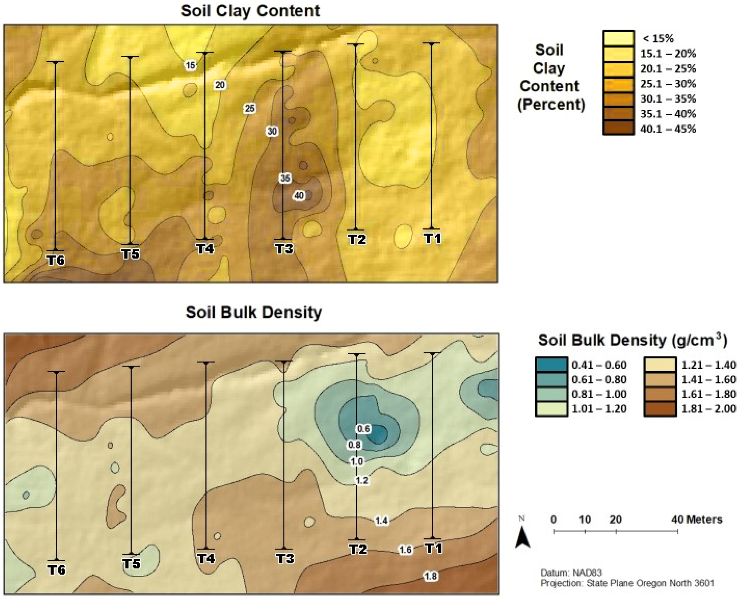
3.2. Soil Characteristics and Moisture Fluctuations

The clay content was generally high along transect 3, but did not seem to clearly correspond to areas of high water content (Figure 1 and Figure 2). In contrast, bulk density variation in the study area indicated corresponding areas of lower bulk density and higher soil water content. The general trend for soil bulk density in the study area indicated an increase with transects from upland (transects 1, 2, and 3) to lowland (transects 4, 5, and 6) (Figure 1).
Although there were clear changes in soil moisture through the year, a pattern of consistently high soil moisture was maintained through the year at the east-central side of the study area (Figure 2). In such areas, soil moisture was never lower than 70%, even during August, the driest month. Variation in soil moisture at the west and central parts of the study area was much more noticeable throughout the year. In those areas, soil moisture was predominantly about 60% during the wettest month (April), and it was about half (30%) during the driest month (August).
Fluctuations in average soil water content during the period of study (February 2019–2020) followed the variations in precipitation in the study area (Figure 3). In general, the wettest period of the year was spring, while the driest period was during late June to mid-September. Soil water content was highest in April (66% to 69%), but not significantly different from that in January (66% to 67%) (Figure 4). October (55% to 61%) and August (36% to 39%) had lower soil moisture.

3.3. Plant Water Stress Responses to Drought

Four representative species were selected to test their physiological response to soil moisture variation during the dry season: J. effusus, J. patens, S. microcarpus, and T. latifolia. The midday water potential of the four species changed significantly (p < 0.05) in response to changes in soil moisture. The two Juncus species experienced lower midday water potentials (up to about −2.5 MPa) and were found in areas with lower soil water content (as low as 27%) (Figure 5) than S. microcarpus and T. latifolia (Figure 6). The latter two species were found in areas with soil moisture no lower than 37%. As expected, the predawn water potential of the four species was less variable than the midday water potential with respect to changes in soil moisture. In the two Juncus species, little change occurred in the predawn water potential with changes in water content, while in the other two species, the predawn water potential varied substantially with soil moisture.

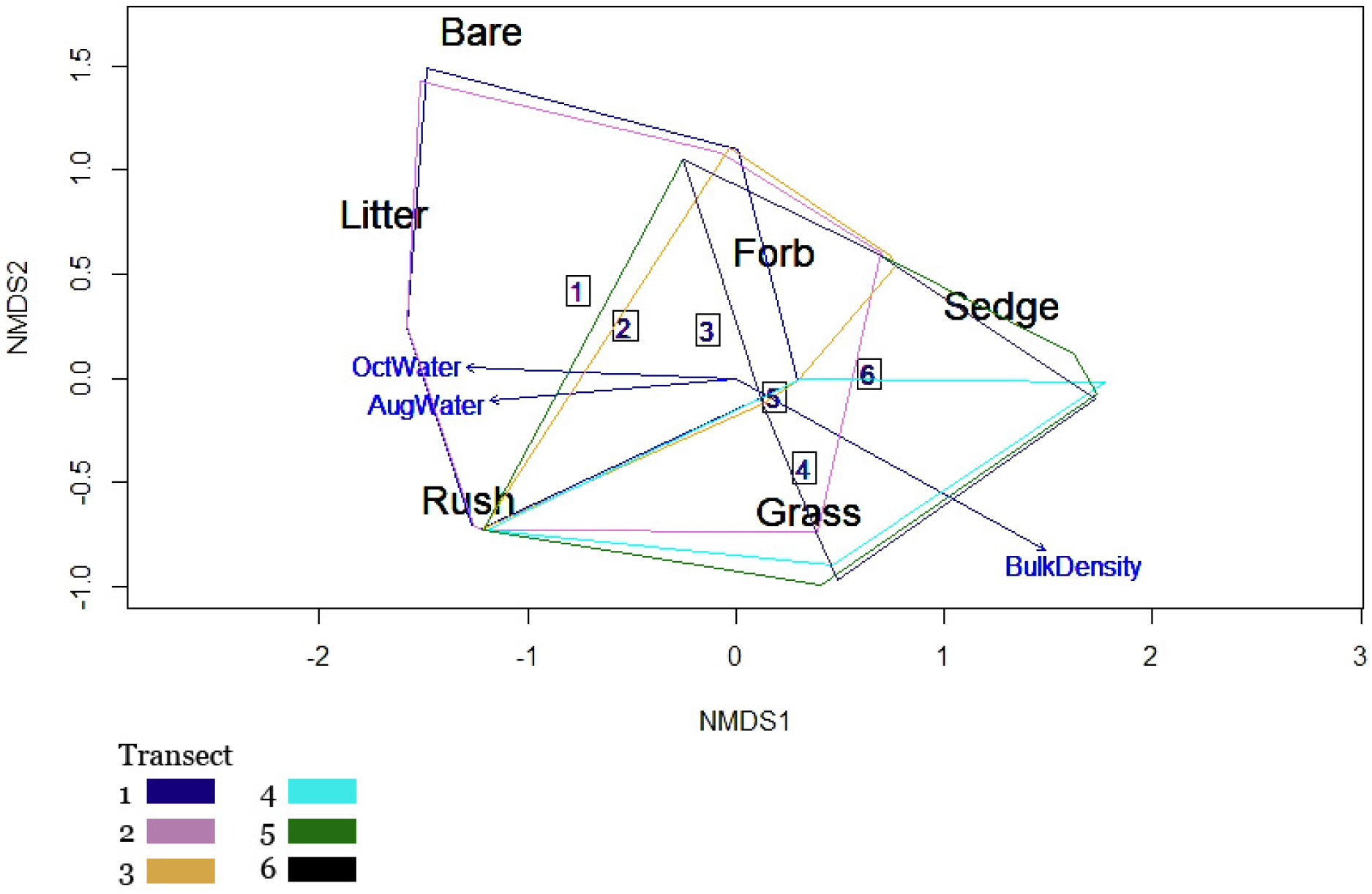
3.4. Functional Group Responses to Soil and Moisture

Soil moisture in August and October as well as bulk density were significant environmental variables correlated with plant community structure of functional groups (Figure 7). The NMDS ordination revealed that the plant community structure of functional groups differed between transects, with transects 1, 2, and 3 consisting more of rushes, litter, and bare ground, while transects 4, 5, and 6 are more likely to be dominated by sedges, grasses, and forbs. We analyzed three soil variables, soil moisture, soil texture, and soil bulk density, to understand their impacts on the distribution of functional groups in the study area. August’s and October’s soil moisture appears to be positively correlated with plant communities associated with transects 1, 2, and 3 (rushes and sedges) (Figure 8), while bulk density is positively correlated with communities in 4, 5, and 6 (grasses and forbs), with the opposite being true for negative correlations.
The double stepwise GLM reduction resulted in models with different explanatory variables for many of the response variables of interest. Sedges, bare ground, and litter models reduced to single explanatory variables, while the grass model was explained by two variables (August moisture and soil bulk density), and the rush model was composed of August soil moisture, bulk density, and clay percentage. Rushes were positively correlated with clay percentage (Figure 8) and August soil moisture, but negatively correlated with soil bulk density. Rushes were also positively correlated with October moisture, but the model was more parsimonious without it; therefore, the variable was removed during stepwise reduction. Grass occurrence was only significantly correlated (positively) with bulk density (Figure 8). Sedges were negatively correlated with average soil moisture in October (Figure 8).

4. Discussion

4.1. Wetland Plant Species Composition

Our objective was to determine the most dominant or characteristic plant species in our study area as the first step to envision suitable conservation or restoration practices. Wetlands support a wide variety of species on a relatively small surface. We found that T. latifolia and S. microcarpus were dominant within transects 1 and 2, which were the transects with higher soil moisture and lower bulk density. Transects 5 and 6 were the driest transects and were dominated by grasses such as A. pratensis and P. arundinacea. However, J. effusus, J. patens, and D. fullonum were found in both wetter and drier transects. These data show the large variability that moisture and soil characteristics can cause in vegetation in a small area. Although our use of functional groups based on growth form has its limitations [24], we believe such grouping is adequate in understanding plant responses.

4.2. Abiotic Factors Affecting Functional Groups

Based on the NMDS ordination and our models, we consider soil moisture, soil texture and soil bulk density as distinguishable contributing factors for spatial variation in plant functional groups (grasses, forbs, sedges, and rushes) in our study area. Many factors have the potential to influence soil volumetric water content such as precipitation events, topographic features, and geographical conditions [25]. The study area has a slight slope, which controls the field-scale spatio-temporal variability of soil moisture [26]. We observed at the downslope that the study site has abundant rock fragments, which are an important factor for measuring lower soil moisture at the downslope transects because of faster water movement [27]. Therefore, we suspect that because of the presence of rock fragments at the downslope, the highest soil moisture was recorded within upslope transects (transects 1 and 2), while transects 5 and 6, located in the downslope site, have the lowest soil moisture.
Based on our data, D. fullonum was found to be the main invasive exotic species in the wetland. This is a biennial forb that prefers moist soil; however, it tolerates dry conditions because it produces a deep taproot [28]. Dipsacus fullonum grows in varying soil textures from loamy sand to heavy clay soils [29], which was confirmed in our study. This is an introduced species from Europe that is considered an invasive weed in North America, as well as in parts of South America [28,30]. Given the adaptability of this species, its management should be focused on maintaining a proper plant cover of native perennial species such as the dominant Juncus species, especially as the seeds of D. fullonum germinate under a broad range of environmental conditions and could compete with regeneration of the native cover under disturbance and decrease diversity [30]. Our results, with D. fullonum dominating the study area in a variety of soil conditions, highlight the need to better understand its biology and potential control. This is especially important as its current dominance may be a direct effect of the past management of the wetland, which included grazing. Finally, understanding the factors that favor this species’ establishment can benefit management practices from multiple areas in which this widely distributed invasive species is invading.
Other species that our study determined to be dependent on high soil moisture included the perennial native species T. latifolia and S. microcarpus, while some other species such as A. pratensis and P. arundinacea were found to be associated with lower soil moisture. Typha latifolia and S. microcarpus may increase soil organic matter more than other plant species, in turn decreasing the bulk density of the soil [31,32,33]. Lower bulk density suggests that there is more pore space available in the soil, which increases the water availability in the soil to be used for plant growth [34]. This is important, as they represent feedback in which both species favor the growth and establishment of the late seral community on which both are present. Conservation efforts should consider maintaining a proper cover of T. latifolia and S. microcarpus to favor the water storage in this and other wetlands in the Willamette Valley.
On the other hand, A. pratensis and P. arundinacea, which were located on the drier areas of the wetland, tolerate both wet and drier conditions [35] and are mainly located on clay or loam soils and the areas of higher bulk density [36], as was indicated by our models, showing that grasses were positively correlated with bulk density. Phalaris arundinacea is a native species [37], but A. pratensis is not and was originally introduced for hay and pasture [38]. Both species can be highly competitive due to their rhizomatous nature and high seed production. Under improper management, both species can become invasive [37].
This study showed that J. effusus, J. patens, and D. fullonum are intermediate species in terms of soil moisture requirements. Therefore, even though J. effusus, and J. patens are wetland plant species, they tolerate changes in soil moisture and fairly dry conditions. Other studies have reported Juncus species tolerating water stress (high in water use efficiency) compared with other wetland species [39,40]. Our finding that rushes were also positively correlated with clay percentage has been corroborated by other studies that found that the Juncus species preferred to grow in clay and loam soils [41]. However, while we found a negative correlation between rushes and bulk density, Ref. [42] found that areas dominated by J. effusus and J. patens had lower organic matter, resulting in higher bulk density.

4.3. Wetland Plant Species Responses to Drought

From the four species evaluated for water stress, we found two general responses: species with higher levels of stress (J. effusus and J. patens), and species with lower levels (T. latifolia and S. microcarpus). The lower stress levels of T. latifolia and S. microcarpus are associated with their presence in areas of the wetland with more moisture, and therefore their dependence on higher soil moisture [43]. This could indicate that a reduction in the wetland’s water storing capacity could have a higher effect on T. latifolia and S. microcarpus. On the other hand, our water potential results indicate that both Juncus species can tolerate higher levels of stress, allowing them to persist if the wetland water storing capacity is reduced in response to disturbance. Furthermore, D. fullonum, P. arundinacea, and A. pratensis were not evaluated for their responses to stress, but are found in the drier areas of the wetland, possibly indicating that all species could spread and invade the wetland under drier conditions since the three species can be invasive [30,37,38].
Conservation efforts that involve maintaining desirable native plant cover in wetlands are important to prevent invasive species from spreading. It is possible that the presence of invasive species in the area was favored by historical excessive livestock grazing. Although currently the area is protected from grazing, the recovery of vegetation may take decades. Based on this, restoration efforts may include (1) maintaining the area excluded to livestock grazing so native vegetation can recover and compete with the invasive species, (2) procuring active elimination of invasive species via mechanical means, and (3) avoiding hydric diversions that negatively affect the water supply to the wetland area.

5. Conclusions

We found high variation in plant species within functional groups (forbs, grasses, rushes, and sedges), as well as how they interact with multiple factors associated with soil and moisture. Most functional groups associated with community structure correlate to soil moisture (particularly during August and October) and to soil texture and bulk density. These correlations might forecast a shift in dominance from sedges to rushes if soil moisture content decreases in future scenarios, resulting in a decrease in ecosystem diversity. Changes in vegetation due to fluctuations in hydrology and livestock grazing are common around the world and are prone to affect sensitive areas like wetlands. Furthermore, the dominance of invasive species is an important indicator of the need for appropriate restoration practices. The invasive D. fullonum was the most dominant invasive species, replacing the native plant community and reducing ecosystem quality. Therefore, we recommend maintaining the area excluded from livestock grazing, avoiding hydric diversions, and establishing native plant species such as Willow spp. to influence succession after grazing exclusion. These practices should contribute to restoring native vegetation structures and ecological functions in deteriorated wetlands.

Author Contributions

Conceptualization, C.G.O. and R.M.-G.; methodology, F.A., C.G.O. and R.M.-G.; software, M.H. and J.S.; validation, D.E.P.-T. and R.M.-G.; formal analysis, F.A.; investigation, F.A.; writing—original draft preparation, F.A.; writing—review and editing, D.E.P.-T. and R.M.-G. All authors have read and agreed to the published version of the manuscript.

Funding

The present work was financed by Oregon State University and the Turkish government through a graduate scholarship to the senior author.

Institutional Review Board Statement

Not applicable.

Informed Consent Statement

Not applicable.

Data Availability Statement

Not applicable.

Acknowledgments

We would like to thank the Turkish General Directorate of Forestry and the Turkish Ministry of National Education for providing financial support.

Conflicts of Interest

The authors declare no conflict of interest.

References

  1. Mitsch, W.; Gosselink, J. Wetlands: Human Use and Science. In Wetlands, 5th ed.; John Wiley & Sons: Hoboken, NJ, USA, 2015; pp. 3–26. [Google Scholar]
  2. Gilmour, D.M.; Butler, V.L.; O’Connor, J.E.; Davis, E.B.; Culleton, B.J.; Kennett, D.J.; Hodgins, G. Chronology and ecology of late Pleistocene megafauna in the northern Willamette Valley, Oregon. Quat. Res. 2015, 83, 127–136. [Google Scholar] [CrossRef]
  3. Fickas, K.C.; Cohen, W.B.; Yang, Z. Landsat-based monitoring of annual wetland change in the Willamette Valley of Oregon, USA from 1972 to 2012. Wetl. Ecol. Manag. 2016, 24, 73–92. [Google Scholar] [CrossRef]
  4. Erwin, K.L. Wetlands and global climate change: The role of wetland restoration in a changing world. Wetl. Ecol. Manag. 2009, 17, 71–84. [Google Scholar] [CrossRef]
  5. Richardson, C.J. Ecological functions and human values in wetlands: A framework for assessing forestry impacts. Wetlands 1994, 14, 1–9. [Google Scholar] [CrossRef]
  6. Faulkner, S.; Barrow, W., Jr.; Keeland, B.; Walls, S.; Telesco, D. Effects of conservation practices on wetland ecosystem services in the Mississippi Alluvial Valley. Ecol. Appl. 2011, 21, S31–S48. [Google Scholar] [CrossRef]
  7. Sueltenfuss, J.P.; Ocheltree, T.W.; Cooper, D.J. Evaluating the realized niche and plant–water relations of wetland species using experimental transplants. Plant Ecol. 2020, 221, 333–345. [Google Scholar] [CrossRef]
  8. Hao, M.; Zhang, J.; Meng, M.; Chen, H.Y.; Guo, X.; Liu, S.; Ye, L. Impacts of changes in vegetation on saturated hydraulic conductivity of soil in subtropical forests. Sci. Rep. 2019, 9, 8372. [Google Scholar] [CrossRef] [PubMed]
  9. Niemuth, N.D.; Wangler, B.; Reynolds, R.E. Spatial and temporal variation in wet areas of wetlands in the prairie pothole region of North Dakota and South Dakota. Wetlands 2010, 30, 1053–1064. [Google Scholar] [CrossRef]
  10. Naumburg, E.; Mata-González, R.; Hunter, R.G.; Mclendon, T.; Martin, D.W. Phreatophytic vegetation and groundwater fluctuations: A review of current research and application of ecosystem response modeling with an emphasis on Great Basin vegetation. Environ. Manag. 2005, 35, 726–740. [Google Scholar] [CrossRef]
  11. Mata-González, R.; Averett, J.P.; Abdallah, M.A.; Martin, D.W. Variations in groundwater level and microtopography influence desert plant communities in shallow aquifer areas. Environ. Manag. 2022, 69, 45–60. [Google Scholar] [CrossRef] [PubMed]
  12. Vivian, S.G. Microtopographic heterogeneity and floristic diversity in experimental wetland communities. J. Ecol. 1997, 1, 71–82. [Google Scholar] [CrossRef]
  13. Reis, V.; Hermoso, V.; Hamilton, S.K.; Ward, D.; Fluet-Chouinard, E.; Lehner, B.; Linke, S. A global assessment of inland wetland conservation status. Bioscience 2017, 67, 523–533. [Google Scholar] [CrossRef]
  14. Bourdeau, P.F. A test of random versus systematic ecological sampling. Ecology 1953, 34, 499–512. [Google Scholar] [CrossRef]
  15. McGarvey, R.; Burch, P.; Matthews, J.M. Precision of systematic and random sampling in clustered populations: Habitat patches and aggregating organisms. Ecol. Appl. 2016, 26, 233–248. [Google Scholar] [CrossRef] [PubMed]
  16. Soil Survey Staff. Natural Resources Conservation Service, United States Department of Agriculture Official Soil Series Descriptions. Available online: http://soils.usda.gov (accessed on 5 February 2020).
  17. Bonham, C.D. Measurements for Terrestrial Vegetation, 2nd ed.; John Wiley & Sons: Fort Collins, CO, USA, 2013. [Google Scholar]
  18. Gee, G.W.; Bauder, J.W. Particle size analysis by hydrometer: A simplified method for routine textural analysis and a sensitivity test of measurement parameters. Soil Sci. Soc. Am. J. 1979, 43, 1004–1007. [Google Scholar] [CrossRef]
  19. Lane, P.W. Generalized linear models in soil science. Eur. J. Soil Sci. 2002, 53, 241–251. [Google Scholar] [CrossRef]
  20. Stroup, W.W. Rethinking the analysis of non-normal data in plant and soil science. Agron. J. 2015, 107, 811–827. [Google Scholar] [CrossRef]
  21. Guan, Y.; Wei, J.; Zhang, D.; Zu, M.; Zhang, L. To identify the important soil properties affecting dinoseb adsorption with statistical analysis. Sci. World J. 2013, 6, 713–721. [Google Scholar] [CrossRef]
  22. Koenker, R.; Machado, J. Goodness of fit and related inference processes for quantile regression. J. Am. Stat. Assoc. 1999, 94, 1296–1310. [Google Scholar] [CrossRef]
  23. Lichvar, R.W.; Banks, D.L.; Kirchner, W.N.; Melvin, N.C. The National Wetland Plant List: 2016 wetland ratings. Phytoneuron 2016, 30, 1–17. [Google Scholar]
  24. Van Bodegom, P.M.; Douma, J.C.; Witte, J.P.; Ordoñez, J.C.; Bartholomeus, R.P.; Aert, R. Going beyond limitations of plant functional types when predicting global ecosystem–atmosphere fluxes: Exploring the merits of traits-based approaches. Glob. Ecol. Biogeogr. 2012, 21, 625–636. [Google Scholar] [CrossRef]
  25. Penna, D.; Tromp-van Meerveld, H.J.; Gobbi, A.; Borga, M.; Dalla Fontana, G. The influence of soil moisture on threshold runoff generation processes in an alpine headwater catchment. Hydrol. Earth Syst. Sci. 2011, 15, 689–702. [Google Scholar] [CrossRef]
  26. Mohanty, B.P.; Skaggs, T.H. Spatio-temporal evolution and time-stable characteristics of soil moisture within remote sensing footprints with varying soil, slope, and vegetation. Adv. Water Resour. 2001, 24, 1051–1067. [Google Scholar] [CrossRef]
  27. Hlaváčiková, H.; Novák, V.; Holko, L. On the role of rock fragments and initial soil water content in the potential subsurface runoff formation. J. Hydrol. Hydromech. 2015, 63, 71–81. [Google Scholar] [CrossRef]
  28. Rector, B.G.; Harizanova, V.; Sforza, R.; Widmer, T.; Wiedenmann, R.N. Prospects for biological control of teasels, Dipsacus spp., a new target in the United States. Biol. Control 2006, 36, 1–14. [Google Scholar] [CrossRef]
  29. Beaton, L.L.; Dudley, S.A. Tolerance of roadside and old field populations of common teasel (Dipsacus fullonum subsp. sylvestris) to salt and low osmotic potentials during germination. AoB Plants 2013, 5, plt001. [Google Scholar] [CrossRef]
  30. Daddario, J.F.; Bentivegna, D.J.; Tucat, G.; Fernandez, O.A. Environmental factors affecting seed germination of common teasel (Dipsacus fullonum). Planta Daninha 2017, 35, 823–832. [Google Scholar] [CrossRef]
  31. Mitchell, M.E.; Lishawa, S.C.; Geddes, P.; Larkin, D.J.; Treering, D.; Tuchman, N.C. Time-dependent impacts of cattail invasion in a Great Lakes coastal wetland complex. Wetlands 2011, 31, 1143–1149. [Google Scholar] [CrossRef]
  32. Wolf, E.; Cooper, D. Restoration of Geomorphic Structure, Hydrologic Regime, and Vegetation in Upper Halstead Meadow; Project Report to Sequoia National Park; Colorado State University: Three Rivers, CA, USA, 2011. [Google Scholar]
  33. Sloey, T.M.; Hester, M.W. Interactions between soil physicochemistry and belowground biomass production in a freshwater tidal marsh. Plant Soil 2016, 401, 397–408. [Google Scholar] [CrossRef]
  34. Czayka, A. Typha Control and Sedge/Grass Meadow Restoration on a Lake Ontario Wetland. Master’s Thesis, SUNY Brockport, Brockport, NY, USA, 2012. [Google Scholar]
  35. Mitchell, J.W.; Livingston, G.A. Methods of Studying Plant Hormones and Growth-Regulating Substances; Agriculture Handbook 336; U.S. Government Printing Office: Washington, DC, USA, 1968. [Google Scholar]
  36. Lillak, R.; Viiralt, R.; Linke, A.; Geherman, V. Integrating efficient grassland farming and biodiversity. In Proceedings of the 13th International Occasional Symposium of the European Grassland Federation, Tartu, Estonia, 29–31 August 2005; Estonian Grassland Society: Tartu, Estonia, 2005. [Google Scholar]
  37. Perry, L.G.; Galatowitsch, S.M.; Rosen, C.J. Competitive control of invasive vegetation: A native wetland sedge suppresses Phalaris arundinacea in carbon-enriched soil. J. Appl. Ecol. 2004, 41, 151–162. [Google Scholar] [CrossRef]
  38. Sheley, R. Tolerance of meadow foxtail (Alopecurus pratensis) to two sulfonylurea herbicides. Weed Technol. 2007, 21, 470–472. [Google Scholar] [CrossRef]
  39. Mata-González, R.; McLendon, T.; Martin, D.W.; Trlica, M.J.; Pearce, R.A. Vegetation as affected by groundwater depth and microtopography in a shallow aquifer area of the Great Basin. Ecohydrology 2012, 5, 54–63. [Google Scholar] [CrossRef]
  40. Evans, T.L.; Mata-González, R.; Martin, D.W.; McLendon, T.; Noller, J.S. Growth, water productivity, and biomass allocation of Great Basin plants as affected by summer watering. Ecohydrology 2013, 6, 713–721. [Google Scholar] [CrossRef]
  41. Les, D.H. Aquatic Dicotyledons of North America: Ecology, Life History, and Systematics, 1st ed.; CRC Press: Boca Raton, FL, USA, 2017. [Google Scholar]
  42. Burdick, D.M.; Roman, C.T. Salt marsh responses to tidal restriction and restoration. In Tidal Marsh Restoration; Island Press: Washington, DC, USA, 2012; pp. 373–382. [Google Scholar]
  43. Li, S.; Pezeshki, S.R.; Goodwin, S. Effects of soil moisture regimes on photosynthesis and growth in cattail (Typha latifolia). Acta Oecol. 2004, 25, 17–22. [Google Scholar] [CrossRef]
Figure 1. Geospatial interpolation of the representative differences in soil clay content (%) and soil bulk density in the study area. The six black straight lines in the figures indicate the location of the transects where sampling occurred within the wetland.
Sustainability 15 14377 g001
Figure 2. Map of the research area displaying the geospatial interpolation of soil volumetric water content in the top 20 cm of the soil profile at different times of the year (2019–2020). The six black straight lines in the figures indicate the location of the transects where sampling occurred within the wetland.
Sustainability 15 14377 g002
Figure 3. Daily precipitation records from the meteorological stations and average weekly soil volumetric water content measurements (0–20 cm depth) obtained during the study period (February 2019–February 2020) at the study area.
Sustainability 15 14377 g003
Figure 4. Soil moisture percentages in April, August, October 2019, and January 2020. Asterisks (***) between seasons indicate comparisons of means from the Wilcoxon rank sum test.
Sustainability 15 14377 g004
Figure 5. Soil water content and water potential relationships for (A) Juncus effusus and (B) Juncus patens. Left panels show midday water potential and right panels show predawn water potential. Solid lines are medians and dashed lines are mean values. All regressions p < 0.05 except as marked in the figure.
Sustainability 15 14377 g005
Figure 6. Soil water content and water potential correlation of (A) Scirpus microcarpus and (B) Typha latifolia. Left panels show midday water potential and right panels show predawn water potential. Solid lines are medians and dashed lines are mean values. All regressions p < 0.05.
Sustainability 15 14377 g006
Figure 7. The distribution of functional groups, soil bulk density, and soil moisture in October and August on six transects. Plotted axes are only the significant correlations (p < 0.05).
Sustainability 15 14377 g007
Figure 8. Correlation between rush cover and clay percentage, grass cover and bulk density, and sedge cover and October soil water percentage. Clay and avg. October soil moisture is %, bulk density is grams per milliliter (g/mL).
Sustainability 15 14377 g008
Table 1. Plants species, life cycles, wetland indicator status, and mean basal vegetation cover for all the six transects. Life cycle categories: P (Perennial), A (Annual), B (Biennial). Wetland indicator status from Lichvar et al. [23]: OBL (Obligate wetland), FACW (Facultative wetland), FAC (Facultative), FACU (Facultative upland), UPL (Obligate upland).
Basal Cover (%)
ForbsCycleStatusT1T2T3T4T5T6
Cirsium arvensePFAC00000.80
Daucus carotaBFACU0004.900
Dipsacus fullonumBFAC20.649.65227.221.541.3
Galium aparineAFACU0.80001.60.8
Leucanthemum vulgarePFACU0000.800
Malva neglectaAFACU00001.60
Myosotis laxaAOBL1.600.81.60.80.82
Typha latifoliaPOBL2.54.90000
Veronica americanaPOBL00.800.800
Vicia sativaAFACU000000.8
Vicia tetraspermaAFACU04.97.411.52.47.4
Grasses
Alopecurus pratensisPFAC1.61.67.430.534.714
Holcus lanatusPFAC1.601.60.82.40.8
Phalaris arundinaceaPFACW0000011.5
Poa pratensisPFAC1.62.40.82.401.6
Rushes
Juncus effususPFACW17.312.46.67.48.24.9
Juncus patensPFACW4.95.82.44.91.60.8
Sedges
Carex amplifoliaPOBL02.50000
Carex densaPOBL00004.10.8
Carex fetaPFACW000.8000
Carex pellitaPOBL00.80009.1
Carex stipataPOBL1.64.113.25.813.23.3
Schoenoplectus acutusPOBL00006.60
Scirpus microcarpusPOBL27.24.90000
Disclaimer/Publisher’s Note: The statements, opinions and data contained in all publications are solely those of the individual author(s) and contributor(s) and not of MDPI and/or the editor(s). MDPI and/or the editor(s) disclaim responsibility for any injury to people or property resulting from any ideas, methods, instructions or products referred to in the content.

