
Using the Life Cycle Approach for Multiobjective Optimization in the Context of the Green Supply Chain: A Case Study of Brazilian Coffee

Abstract
:1. Introduction
- -
- Check the feasibility of performing multiobjective optimization mainly under the life cycle perspective.
- -
- Understand the behavior of a supply chain more clearly when considering the environmental variable, even when it comes to the limit situation to distrust the economic variable.
- -
- To help managers, farmers, retailers, and other stakeholders that act in the manufacturing chain of national coffee to develop cost reduction strategies and meet the (growing) demands for the product’s environmental sustainability.
2. Materials and Methods
2.1. General Aspects Related to Brazilian Coffee and the American Consumer Market
2.2. Environmental and Economic Life Cycle Modeling
2.3. Optimization Modeling
3. Results and Discussion
3.1. Environmental Analysis: Life Cycle Assessment Results
3.2. Optimization Results
4. Conclusions
- -
- Confirming reports available in the literature by pointing out coffee cultivation as the stage that concentrates the most significant contributions to the Global Warming Potential of the entire arrangement.
- -
- The transport of the product by road also plays an essential role in the same context, especially if the distances to be covered during the journey port–roaster–consumer center in the United States are extensive.
- -
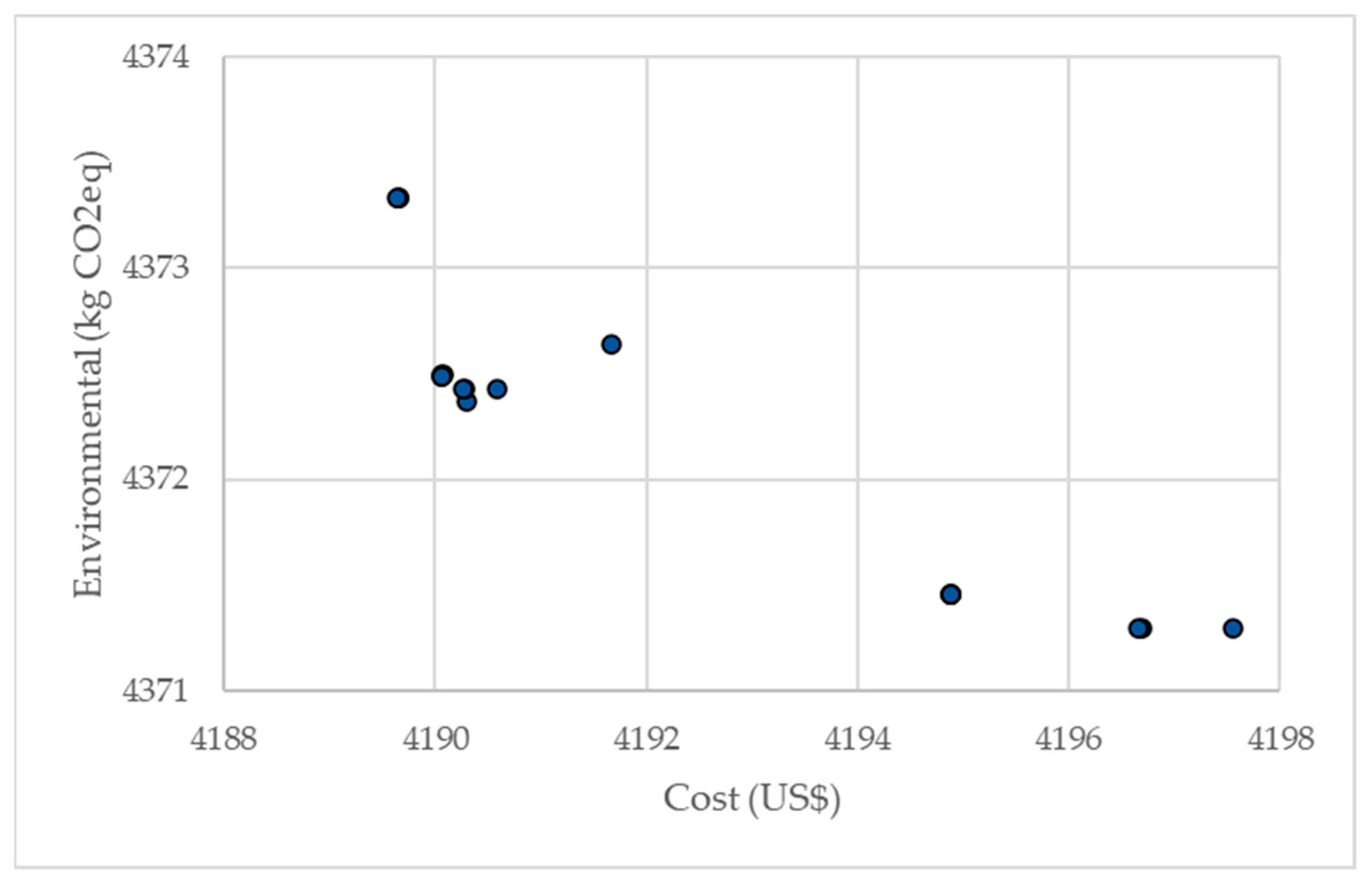
- These are competing objectives.
- -
- Considering environmental aspects for supply chain management can bring non-trivial results, with the boundary condition of a monopoly ensuring the possible environmental performance.
- -
- One of these possibilities comprises modifying specific variables and restrictions that make up the current MOO model to consider uncertainties related to them. One way of approaching the issue is to proceed as Torabzadeh et al. [11] and model part of the data using fuzzy logic. In this way, vital parameters for the model, such as the demand for coffee in the United States, agricultural productivity in Brazil, and the price of green coffee quoted on the stock exchange, could be contemplated more realistically.
- -
- Expanding coffee production and consumption markets and incorporating other regions of the planet would be another natural outcome of this study. Acting in this way opens the prospect, for example, of verifying the influence between these centers in the case of excess supply or demand. Another variant of the current issue consists of identifying the installation location of a roaster capable of absorbing the variations in coffee demand that occur in the United States. A sensitivity analysis involving the loss resulting from the roasting process could also highlight the importance of having more efficient industries in the global SC scenario.
- -
- Investigating the environmental and economic validity of scenarios in which coffee grinding and roasting occurs in Brazil instead of in America. Morita et al. [58] had already used this approach to evaluate the environmental performance of jeans commercialized in the Brazilian market but produced with inputs imported from the United States. This approach would serve to verify if the environmental impacts could be reduced. Additionally, and maybe with more relevance, the analysis would help create a value chain capable of raising economic income in a developing country.
- -
- In the context of carbon taxation, it would be possible to evaluate the impact of this policy, considering that agricultural cultivation and industrial activity can have positive and negative effects on the cost of coffee. Chaudhari et al. [59] followed this direction when exploring such a variant.
- -
- Finally, it would still be possible to integrate the social variable with the present model of MOO, converting the exercise of GSCM into an SSCM.
Author Contributions
Funding
Institutional Review Board Statement
Informed Consent Statement
Data Availability Statement
Conflicts of Interest
Abbreviations
| Glossary | |
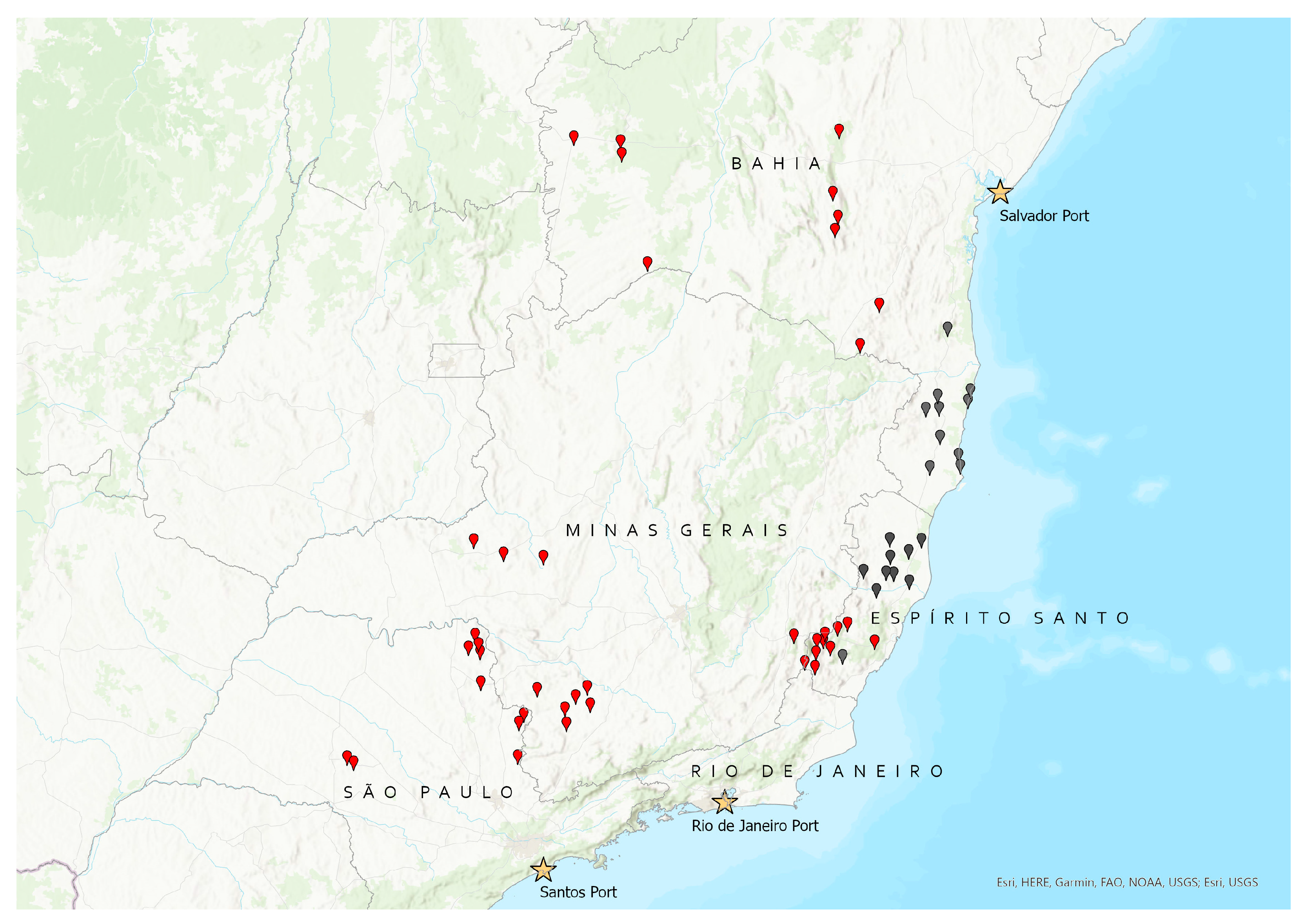
| i | Coffee-producing regions in Brazil: Bahia (BA): Arabica and Robusta varieties; Espírito Santo (ES): Arabica and Robusta; São Paulo (SP): Arabica; and Minas Gerais (MG): Arabica |
| j | Port of origin in Brazil: Santos (SP); Rio de Janeiro (RJ); and Salvador (BA) |
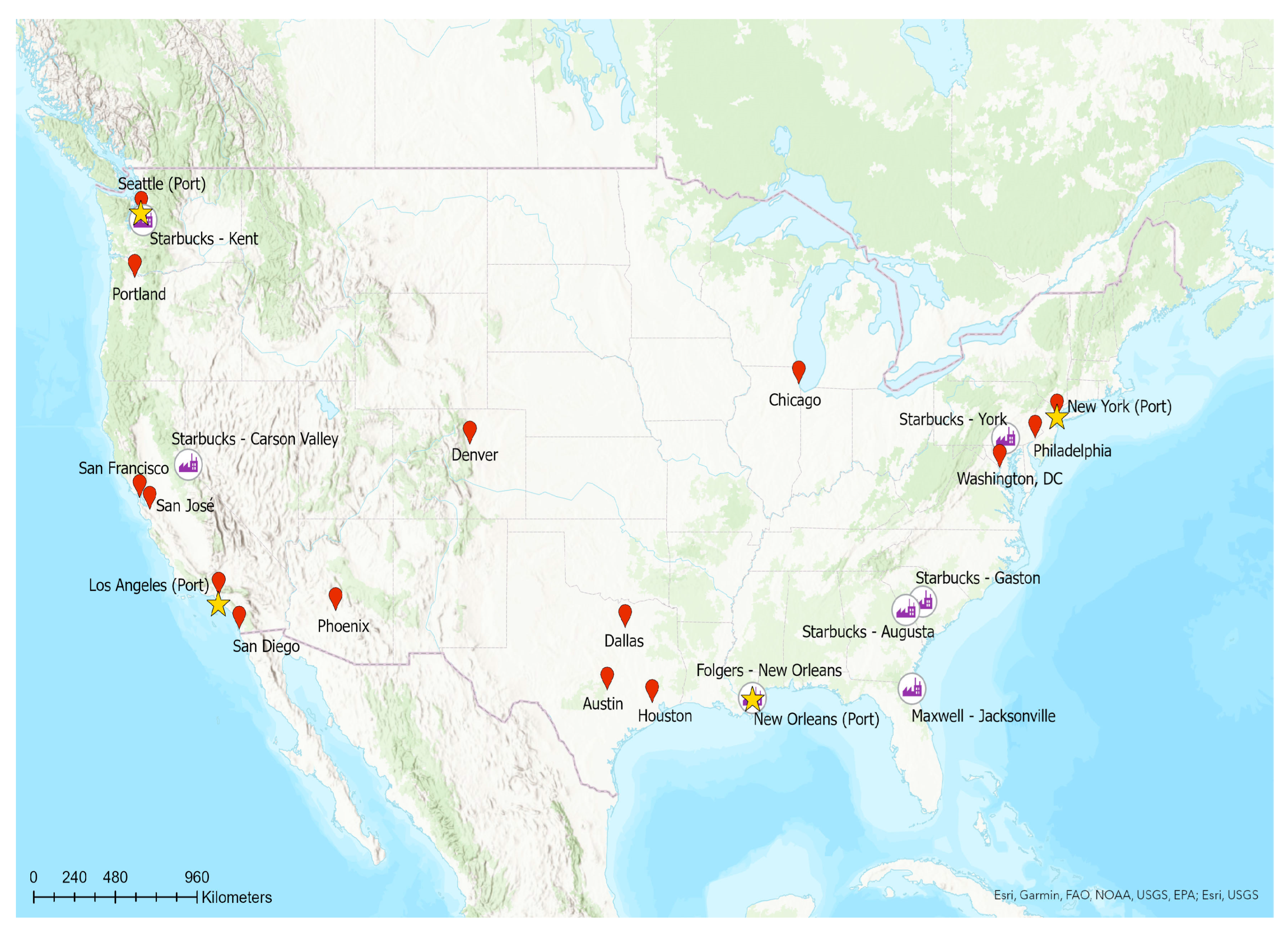
| m | Port of destination in the United States: New York (NJ); New Orleans (LA); Los Angeles (CA); and Seattle (WA) |
| n | Coffee roasters in the United States: Folgers; Maxwell; Starbucks Augusta; Starbucks Gaston; Starbucks Carson Valley; Starbucks Kent; and Starbucks York |
| p | Coffee-consuming cities in the United States: New York (NJ); Los Angeles (CA); Chicago (IL); San Francisco (CA); Seattle (WA); San Diego (CA); Houston (TX); Philadelphia (PA); Portland (OR); Washington (DC); San Jose (CA); Phoenix (AZ); Austin (TX); Denver (CO); and Dallas (TX) |
| Variables | |
| xij | Average distance traveled between the coffee growing area and the port of origin (km) |
| yij | Amount of coffee shipped from the producer to the port of origin (kg) |
| zjm | Amount of coffee shipped from the port of origin (Brazil) to the port of destination (US) (kg) |
| wmn | Quantity of coffee shipped from the American port to the roasting company (kg) |
| knp | Amount of coffee shipped from the roaster to the consumer center (kg) |
References
- Food and Agriculture Organization of the United Nations. Coffee. Available online: https://www.fao.org/markets-and-trade/commodities/coffee/en/ (accessed on 8 March 2023).
- Statista Coffee—Worldwide. Available online: https://www.statista.com/outlook/cmo/hot-drinks/coffee/worldwide (accessed on 8 March 2023).
- International Coffee Organization. Coffee Production by Exporting Countries. Available online: https://www.ico.org/prices/po-production.pdf (accessed on 14 August 2023).
- International Coffee Organization. Imports of Coffee by Selected Importing Countries. Available online: https://www.ico.org/prices/m4-imports.pdf (accessed on 14 August 2023).
- Sachs, J.D.; Cordes, K.; Rising, J.; Toledano, P.; Maennling, N. Ensuring Economic Viability and Sustainability of Coffee Production. 2020. Available online: https://scholarship.law.columbia.edu/cgi/viewcontent.cgi?article=1052&context=sustainable_investment_staffpubs (accessed on 11 September 2023).
- International Coffee Organization. Impact of COVID-19 on the Global Coffee Sector: Survey of ICO Exporting Members. 2020. Available online: https://www.ico.org/documents/cy2019-20/coffee-break-series-3e.pdf (accessed on 11 September 2023).
- Pham, Y.; Reardon-Smith, K.; Mushtaq, S.; Cockfield, G. The Impact of Climate Change and Variability on Coffee Production: A Systematic Review. Clim. Change 2019, 156, 609–630. [Google Scholar] [CrossRef]
- Clavijo-Buritica, N.; Triana-Sanchez, L.; Escobar, J.W. A Hybrid Modeling Approach for Resilient Agri-Supply Network Design in Emerging Countries: Colombian Coffee Supply Chain. Socioecon. Plann. Sci. 2023, 85, 101431. [Google Scholar] [CrossRef]
- Barreto Peixoto, J.A.; Silva, J.F.; Oliveira, M.B.P.P.; Alves, R.C. Sustainability Issues along the Coffee Chain: From the Field to the Cup. Compr. Rev. Food Sci. Food Saf. 2023, 22, 287–332. [Google Scholar] [CrossRef] [PubMed]
- Christopher, M. Logistics and Supply Chain Management: Creating Value-Adding Networks, 3rd ed.; FT Prentice Hall: Upper Saddle River, NJ, USA, 2005. [Google Scholar]
- Torabzadeh, S.A.; Nejati, E.; Aghsami, A.; Rabbani, M. A Dynamic Multi-Objective Green Supply Chain Network Design for Perishable Products in Uncertain Environments, the Coffee Industry Case Study. Int. J. Manag. Sci. Eng. Manag. 2022, 17, 220–237. [Google Scholar] [CrossRef]
- Barbosa-Póvoa, A.P. Process Supply Chains Management—Where Are We? Where to Go Next? Front. Energy Res. 2014, 2, 23. [Google Scholar] [CrossRef]
- Zhang, Q.; Shah, N.; Wassick, J.; Helling, R.; van Egerschot, P. Sustainable Supply Chain Optimization: An Industrial Case Study. Comput. Ind. Eng. 2014, 74, 68–83. [Google Scholar] [CrossRef]
- Asha, L.N.; Dey, A.; Yodo, N.; Aragon, L.G. Optimization Approaches for Multiple Conflicting Objectives in Sustainable Green Supply Chain Management. Sustainability 2022, 14, 12790. [Google Scholar] [CrossRef]
- Jayarathna, C.P.; Agdas, D.; Dawes, L.; Yigitcanlar, T. Multi-Objective Optimization for Sustainable Supply Chain and Logistics: A Review. Sustainability 2021, 13, 13617. [Google Scholar] [CrossRef]
- Sakamoto, H.; Ronquim, F.M.; Seckler, M.M.; Kulay, L. Environmental performance of effluent conditioning systems for reuse in oil refining plants: A case study in Brazil. Energies 2019, 12, 326. [Google Scholar] [CrossRef]
- Azapagic, A.; Clift, R. Life Cycle Assessment and Multiobjective Optimization. J. Clean. Prod. 1999, 7, 135–143. [Google Scholar] [CrossRef]
- Azapagic, A.; Clift, R. The Application of Life Cycle Assessment to Process Optimization. Comput. Chem. Eng. 1999, 23, 1509–1526. [Google Scholar] [CrossRef]
- Salomone, R. Life Cycle Assessment Applied to Coffee Production: Investigating Environmental Impacts to Aid Decision Making for Improvements at Company Level. J. Food Agric. Environ. 2003, 1, 295–300. [Google Scholar]
- Giraldi-Díaz, M.R.; De Medina-Salas, L.; Castillo-González, E.; León-Lira, R. Environmental Impact Associated with the Supply Chain and Production of Grounding and Roasting Coffee through Life Cycle Analysis. Sustainability 2018, 10, 4598. [Google Scholar] [CrossRef]
- Phrommarat, B. Life Cycle Assessment of Ground Coffee and Comparison of Different Brewing Methods: A Case Study of Organic Arabica Coffee in Northern Thailand. Environ. Nat. Resour. J. 2019, 17, 96–108. [Google Scholar] [CrossRef]
- Nab, C.; Maslin, M. Life Cycle Assessment Synthesis of the Carbon Footprint of Arabica Coffee: Case Study of Brazil and Vietnam Conventional and Sustainable Coffee Production and Export to the United Kingdom. Geo 2020, 7, e00096. [Google Scholar] [CrossRef]
- Usva, K.; Sinkko, T.; Silvenius, F.; Riipi, I.; Heusala, H. Carbon and Water Footprint of Coffee Consumed in Finland—Life Cycle Assessment. Int. J. Life Cycle Assess. 2020, 25, 1976–1990. [Google Scholar] [CrossRef]
- Brenes-Peralta, L.; De Menna, F.; Vittuari, M. Interlinked Driving Factors for Decision-Making in Sustainable Coffee Production. Environ. Dev. Sustain. 2022, 1–34. [Google Scholar] [CrossRef]
- Baratsas, S.G.; Pistikopoulos, E.N.; Avraamidou, S. A Systems Engineering Framework for the Optimization of Food Supply Chains under Circular Economy Considerations. Sci. Total Environ. 2021, 794, 148726. [Google Scholar] [CrossRef]
- CONAB—Companhia Nacional de Abastecimento. Portal de Informações Agropecuárias. Available online: https://portaldeinformacoes.conab.gov.br/produtos-360.html (accessed on 26 April 2023). (In Portuguese)
- Brasil—Ministério da Economia. Comex Stat—Exportação e Importação Geral. Available online: http://comexstat.mdic.gov.br/pt/geral (accessed on 20 April 2023). (In Portuguese)
- Statista. Sales of the Leading Regular Ground Coffee Brands in the United States in 2020. Available online: https://www.statista.com/statistics/188315/top-ground-coffee-brands-in-the-united-states/ (accessed on 27 April 2023).
- Goldberg, E. Folger’s Coffee. Commodity Chain Analysis. Available online: https://storymaps.arcgis.com/stories/fe3761cf11454545b2a380cfe77a058a (accessed on 23 April 2023).
- Basch, M. Future of Maxwell House Remains Uncertain. Available online: https://www.jaxdailyrecord.com/news/2020/feb/27/future-of-maxwell-house-remains-uncertain/ (accessed on 27 April 2023).
- Starbucks. Manufacturing & Distribution: Starbucks Coffee Company. Available online: https://www.starbucks.com/careers/find-a-job/manufacturing-and-distribution/ (accessed on 27 April 2023).
- Travis, S. The 50 Most Caffeinated Cities in America. Available online: https://bestlifeonline.com/caffeinated-cities/ (accessed on 27 April 2023).
- ISO14044:2006; Environmental Management—Life Cycle Assessment—Requirements and Guidelines. ISO—International Organization for Standardization: Geneva, Switzerland, 2006.
- Nemecek, T.; Bengoa, X.; Lansche, J.; Roesch, A.; Faist-Emmenegger, M.; Rossi, V.; Humbert, S. Methodological Guidelines for the Life Cycle Inventory of Agricultural Products; Version 3.5; World Food LCA Database (WFLDB); Quantis and Agroscope: Lausanne, Switzerland; Zurich, Switzerland, 2019. [Google Scholar]
- Coltro, L.; Mourad, A.L.; Oliveira, P.A.P.L.V.; Baddini, J.P.O.A.; Kletecke, R.M. Environmental Profile of Brazilian Green Coffee. Int. J. Life Cycle Assess. 2006, 11, 16–21. [Google Scholar] [CrossRef]
- Dones, R.; Bauer, C.; Bolliger, R.; Burger, B.; Faist Emmenegger, M.; Frischknecht, R.; Heck, T.; Jungbluth, N.; Röder, A. Life Cycle Inventories of Energy Systems: Results for Current Systems in Switzerland and other UCTE Countries; Final Report Ecoinvent data v2.0, No. 5; Swiss Centre for Life Cycle Inventories: Dübendorf, Switzerland, 2007. [Google Scholar]
- Empresa de Pesquisa Energética. Balanço Energético Nacional 2021: Ano Base 2020; Rio de Janeiro, Brazil. 2021. Available online: https://www.epe.gov.br/sites-pt/publicacoes-dados-abertos/publicacoes/PublicacoesArquivos/publicacao-601/topico-596/BEN2021.pdf (accessed on 20 April 2023).
- Google Maps. Available online: https://www.google.com/maps (accessed on 10 April 2023).
- SeaRates. Available online: https://www.searates.com/services/distances-time/ (accessed on 13 April 2023).
- Myhre, G.; Shindell, D.; Bréon, F.-M.; Collins, W.; Fuglestvedt, J.; Huang, J.; Koch, D.; Lamarque, J.-F.; Lee, D.; Mendoza, B.; et al. Anthropogenic and Natural Radiative Forcing. In Climate Change 2013: The Physical Science Basis. Contribution of Working Group I to the Fifth Assessment Report of the Intergovernmental Panel on Climate Change; Stocker, T.F., Qin, D., Plattner, G.-K., Tignor, M., Allen, S.K., Boschung, J., Nauels, Y., Xia, Y., Bex, V., Midgley, P.M., Eds.; Cambridge University Press: Cambridge, UK, 2013; pp. 659–740. [Google Scholar]
- Sanchez Moore, C.; Kulay, L. Effect of the Implementation of Carbon Capture Systems on the Environmental, Energy, and Economic Performance of the Brazilian Electricity Matrix. Energies 2019, 12, 331. [Google Scholar] [CrossRef]
- Grodzevich, O.; Romanko, O. Normalization and Other Topics in Multi-Objective Optimization. In Proceedings of the Fields MITACS Industrial Problems Workshop, Toronto, ON, Canada, 14–18 August 2006. [Google Scholar]
- Steuer, R.E. Multiple Criteria Optimization: Theory, Computation, and Application; Krieger: Malabar, FL, USA, 1989. [Google Scholar]
- De Oliveira, L.S.; Saramago, S.F.P. Multiobjective Optimization Techniques Applied to Engineering Problems. J. Braz. Soc. Mech. Sci. Eng. 2010, 32, 94–105. [Google Scholar] [CrossRef]
- Centro de Estudos Avançados em Economia Aplicada—CEPEA-Esalq/USP. Café. Available online: https://www.cepea.esalq.usp.br/br/indicador/cafe.aspx (accessed on 27 April 2023). (In Portuguese).
- Brasil. Diário Oficial da União, Resolução N. 5959, de 20 de Janeiro de 2022. 2022. Available online: https://www.in.gov.br/en/web/dou/-/resolucao-n-5.959-de-20-de-janeiro-de-2022-375504795 (accessed on 14 August 2023). (In Portuguese)
- Cecafé—Conselho dos Exportadores de Café do Brasil. Relatório Mensal Setembro 2021. Available online: https://www.abics.com.br/?jet_download=798 (accessed on 14 August 2023). (In Portuguese).
- Decker, A. Com Custo Marítimo Alto, Café Especial Do Brasil Viaja de Avião. Jornal O Estado de São Paulo, 2 October 2021. Available online: https://economia.uol.com.br/noticias/estadao-conteudo/2021/10/02/com-custo-maritimo-alto-cafe-especial-do-brasil-viaja-de-aviao.htm (accessed on 20 April 2023). (In Portuguese).
- TCI Business Capital Current Freight Rates—July 2022. Available online: https://www.tcicapital.com/tci-insights/current-freight-trends/ (accessed on 29 September 2022).
- Bynum, M.L.; Hackebeil, G.A.; Hart, W.E.; Laird, C.D.; Nicholson, B.L.; Siirola, J.D.; Watson, J.-P.; Woodruff, D.L. Pyomo—Optimization Modeling in Python, 3rd ed.; Springer: Berlin/Heidelberg, Germany, 2021; Volume 67. [Google Scholar]
- Hart, W.E.; Watson, J.P.; Woodruff, D.L. Pyomo: Modeling and Solving Mathematical Programs in Python. Math. Program. Comput. 2011, 3, 219–260. [Google Scholar] [CrossRef]
- Wächter, A.; Biegler, L.T. On the implementation of an interior-point filter line-search algorithm for large-scale nonlinear programming. Math. Program. 2005, 106, 25–57. [Google Scholar] [CrossRef]
- Tavares, M.P.d.F.; Mourad, A.L. Coffee Beverage Preparation by Different Methods from an Environmental Perspective. Int. J. Life Cycle Assess. 2020, 25, 1356–1367. [Google Scholar] [CrossRef]
- Mouron, P.; Bengoa, X.; Riedener, E.; Rossi, V.; Lansche, J. Modelling Documentation for Crop Production, Version 3.1 for Ecoinvent; World Food LCA Database (WFLDB); Quantis and Agroscope: Lausanne, Switzerland; Zurich, Switzerland, 2017. [Google Scholar]
- Jakob, W.; Blume, C. Pareto Optimization or Cascaded Weighted Sum: A Comparison of Concepts. Algorithms 2014, 7, 166–185. [Google Scholar] [CrossRef]
- CONAB—Companhia Nacional de Abastecimento. Acompanhamento da Safra Brasileira: Café—Safra 2022, 4o Levantamento; 2022. Available online: https://www.conab.gov.br/info-agro/safras/cafe/boletim-da-safra-de-cafe (accessed on 20 April 2023). (In Portuguese)
- Byrnes, W.H. (Texas A&M University, School of Law, Fort Worth, TX, USA); Khodakarami, N. (Texas A&M University, School of Agriculture, College Station, TX, USA); Perez, C.N. (Texas A&M University, Bush School of Government, College Station, TX, USA). The Value Chain: A Study of the Coffee Industry. 2016; (Unpublished work).
- Morita, A.M.; Moore, C.C.S.; Nogueira, A.R.; Kulay, L.; da Ravagnani, M.A.S.S. Assessment of Potential Alternatives for Improving Environmental Trouser Jeans Manufacturing Performance in Brazil. J. Clean. Prod. 2020, 247, 119156. [Google Scholar] [CrossRef]
- Chaudhari, U.; Bhadoriya, A.; Jani, M.Y.; Sarkar, B. A generalized payment policy for deteriorating items when demand depends on price, stock, and advertisement under carbon tax regulations. Math. Comput. Simul. 2023, 207, 556–574. [Google Scholar] [CrossRef]


| Brazilian State | Variety of Coffee | Production Year | ||||
|---|---|---|---|---|---|---|
| 2018 | 2019 | 2020 | 2021 | 2022 (1) | ||
| Minas Gerais (MG) | Arabica | 32,970 | 24,235 | 34,337 | 21,859 | 26,687 |
| São Paulo (SP) | Arabica | 6302 | 4340 | 6181 | 4007 | 4886 |
| Bahia (BA) | Arabica | 1880 | 1200 | 1867 | 1229 | 1704 |
| Robusta | 2670 | 1800 | 2120 | 2240 | 2256 | |
| Espírito Santo (ES) | Arabica | 4751 | 3002 | 4765 | 2945 | 4250 |
| Robusta | 8988 | 10,496 | 9193 | 11,221 | 11,600 | |
| Total Brazil | Arabica | 47,484 | 34,296 | 48,737 | 31,424 | 38,784 |
| Robusta | 14,174 | 15,013 | 14,311 | 16,293 | 16,959 | |
| Consumption Center | GWP (kg CO2eq) | O3F, HH (g NO xeq) | FPMF (g PM2.5eq) | O3F, TE (g NO xeq) | TEcoT (kg 1,4-DB) | MEcoT (g 1,4-DB) | HCTox (g 1,4-DB) | MRS (g Cu eq) | FRS (kg oil eq) |
|---|---|---|---|---|---|---|---|---|---|
| Austin | 6.19 | 26.3 | 17.0 | 27.1 | 20.8 | 535 | 424 | 29.1 | 0.89 |
| Chicago | 6.25 | 26.5 | 17.1 | 27.3 | 21.7 | 538 | 428 | 29.2 | 0.91 |
| Dallas | 6.17 | 26.3 | 17.0 | 27.1 | 20.5 | 535 | 423 | 29.1 | 0.89 |
| Denver | 6.37 | 27.1 | 17.2 | 27.9 | 23.2 | 542 | 436 | 29.5 | 0.95 |
| Houston | 6.14 | 26.2 | 17.0 | 27.0 | 20.0 | 533 | 420 | 29.0 | 0.87 |
| Los Angeles | 6.48 | 27.4 | 17.3 | 28.2 | 24.8 | 546 | 443 | 29.7 | 0.99 |
| New York | 6.19 | 26.3 | 17.0 | 27.1 | 20.8 | 535 | 424 | 29.1 | 0.89 |
| Philadelphia | 6.17 | 26.2 | 17.0 | 27.0 | 20.5 | 534 | 422 | 29.1 | 0.88 |
| Phoenix | 6.41 | 27.2 | 17.3 | 28.0 | 23.8 | 544 | 439 | 29.6 | 0.97 |
| Portland | 6.56 | 27.7 | 17.4 | 28.6 | 25.8 | 549 | 448 | 29.9 | 1.02 |
| San Diego | 6.47 | 27.3 | 17.3 | 28.2 | 24.6 | 546 | 442 | 29.7 | 0.99 |
| San Francisco | 6.55 | 27.6 | 17.4 | 28.4 | 25.7 | 549 | 448 | 29.8 | 1.01 |
| San Jose | 6.54 | 27.5 | 17.4 | 28.4 | 25.6 | 548 | 447 | 29.8 | 1.01 |
| Seattle | 6.56 | 27.7 | 17.5 | 28.6 | 25.9 | 549 | 449 | 29.9 | 1.02 |
| Washington DC | 6.13 | 26.1 | 16.9 | 26.9 | 19.9 | 533 | 420 | 29.0 | 0.87 |
Disclaimer/Publisher’s Note: The statements, opinions and data contained in all publications are solely those of the individual author(s) and contributor(s) and not of MDPI and/or the editor(s). MDPI and/or the editor(s) disclaim responsibility for any injury to people or property resulting from any ideas, methods, instructions or products referred to in the content. |
© 2023 by the authors. Licensee MDPI, Basel, Switzerland. This article is an open access article distributed under the terms and conditions of the Creative Commons Attribution (CC BY) license (https://creativecommons.org/licenses/by/4.0/).
Share and Cite
Sakamoto, H.; Bruschi, L.T.; Kulay, L.; Yamakami, A. Using the Life Cycle Approach for Multiobjective Optimization in the Context of the Green Supply Chain: A Case Study of Brazilian Coffee. Sustainability 2023, 15, 13987. https://doi.org/10.3390/su151813987
Sakamoto H, Bruschi LT, Kulay L, Yamakami A. Using the Life Cycle Approach for Multiobjective Optimization in the Context of the Green Supply Chain: A Case Study of Brazilian Coffee. Sustainability. 2023; 15(18):13987. https://doi.org/10.3390/su151813987
Chicago/Turabian StyleSakamoto, Hugo, Larissa Thaís Bruschi, Luiz Kulay, and Akebo Yamakami. 2023. "Using the Life Cycle Approach for Multiobjective Optimization in the Context of the Green Supply Chain: A Case Study of Brazilian Coffee" Sustainability 15, no. 18: 13987. https://doi.org/10.3390/su151813987