Article

Investigation of Landslide Susceptibility Decision Mechanisms in Different Ensemble-Based Machine Learning Models with Various Types of Factor Data

1
College of Geomatics and Geoinformation, Guilin University of Technology, 319 Yanshan Street, Guilin 541006, China
2
Guangxi Key Laboratory of Spatial Information and Geomatics, 319 Yanshan Street, Guilin 541006, China
*
Author to whom correspondence should be addressed.
Sustainability 2023, 15(18), 13563; https://doi.org/10.3390/su151813563
Submission received: 28 July 2023 / Revised: 20 August 2023 / Accepted: 28 August 2023 / Published: 11 September 2023
(This article belongs to the Topic Natural Hazards and Disaster Risks Reduction)

Abstract

:
Machine learning (ML)-based methods of landslide susceptibility assessment primarily focus on two dimensions: accuracy and complexity. The complexity is not only influenced by specific model frameworks but also by the type and complexity of the modeling data. Therefore, considering the impact of factor data types on the model’s decision-making mechanism holds significant importance in assessing regional landslide characteristics and conducting landslide risk warnings given the achievement of good predictive performance for landslide susceptibility using excellent ML methods. The decision-making mechanism of landslide susceptibility models coupled with different types of factor data in machine learning methods was explained in this study by utilizing the Shapley Additive exPlanations (SHAP) method. Furthermore, a comparative analysis was carried out to examine the differential effects of diverse data types for identical factors on model predictions. The study area selected was Cenxi, Guangxi, where a geographic spatial database was constructed by combining 23 landslide conditioning factors with 214 landslide samples from the region. Initially, the factors were standardized using five conditional probability models, frequency ratio (FR), information value (IV), certainty factor (CF), evidential belief function (EBF), and weights of evidence (WOE), based on the spatial arrangement of landslides. This led to the formation of six types of factor databases using the initial data. Subsequently, two ensemble-based ML methods, random forest (RF) and XGBoost, were utilized to build models for predicting landslide susceptibility. Various evaluation metrics were employed to compare the predictive capabilities of different models and determined the optimal model. Simultaneously, the analysis was conducted using the interpretable SHAP method for intrinsic decision-making mechanisms of different ensemble-based ML models, with a specific focus on explaining and comparing the differential impacts of different types of factor data on prediction results. The results of the study illustrated that the XGBoost-CF model constructed with CF values of factors not only exhibited the best predictive accuracy and stability but also yielded more reasonable results for landslide susceptibility zoning, and was thus identified as the optimal model. The global interpretation results revealed that slope was the most crucial factor influencing landslides, and its interaction with other factors in the study area collectively contributed to landslide occurrences. The differences in the internal decision-making mechanisms of models based on different data types for the same factors primarily manifested in the extent of influence on prediction results and the dependency of factors, providing an explanation for the performance of standardized data in ML models and the reasons behind the higher predictive performance of coupled models based on conditional probability models and ML methods. Through comprehensive analysis of the local interpretation results from different models analyzing the same sample with different sample characteristics, the reasons for model prediction errors can be summarized, thereby providing a reference framework for constructing more accurate and rational landslide susceptibility models and facilitating landslide warning and management.

1. Introduction

Landslides rank among the most devastating geological perils globally, characterized by their wide distribution, frequent occurrence, and high destructiveness [1]. The ecological environment incurs significant damage due to frequent geological disasters, and there are considerable losses to agricultural and industrial production and people’s lives and property [2]. According to data released by the China Geological Survey, there were 4810 landslides in China during 2020, marking an increase of 590 compared to 2019. These landslides constituted 61.35% of the overall count of geological disasters [3]. Therefore, in light of the growing occurrence of landslide catastrophes, constructing accurate and reliable landslide susceptibility maps (LSMs) is essential for regional landslide susceptibility assessment and risk analysis [4,5]. An LSM generally refers to a model that accurately predicts the study area that determines the landslide susceptibility index (LSI) by examining the relationship between the location of known landslide areas and the factors that contribute to landslides. This analysis generates a probability map showing the likelihood of landslides occurring throughout the entire study area [6]. The LSI calculates the likelihood of a landslide happening in a particular area by using a nonlinear combination of various environmental factors. Thus, an LSM serves as the foundation for studying landslide risks and finds wide applications in urban planning, early disaster prevention, and other fields, providing a reliable theoretical basis for regional planning, disaster prevention, and mitigation.
Due to the ongoing advancements in computer science, as well as geographic information systems, remote sensing technology, and related disciplines, the approaches used for studying landslide susceptibility have transitioned from qualitative and semi-quantitative to quantitative analysis [7]. Abundant expert experience is typically required for qualitative and semi-quantitative analysis methods, such as expert scoring and the analytic hierarchy process (AHP), to determine the likelihood of a landslide event occurring [8,9]. Nevertheless, these approaches heavily depend on subjective prior knowledge, and in cases where expert opinions prove to be erroneous, the resulting calculations may diverge from objective reality [10]. Driven by data, methods of quantitative analysis are more practical for assessing susceptibility to landslide disasters. These methods primarily utilize physical–mechanical, conditional probability, and machine learning (ML) models to reflect the correlation between occurrences of landslides and the factors that contribute to them [11]. Physical–mechanical models calculate and analyze the mechanism of landslide occurrence based on geological and topographical parameters obtained through field investigations in landslide-prone areas [12]. They have the advantages of clear physical meaning and accurate analysis results. However, they require many geological and hydrological parameters and are only suitable for analyzing specific types of landslides on a small scale [13]. Common conditional probability models include frequency ratio (FR), information value (IV), certainty factor (CF), evidential belief function (EBF), and weights of evidence (WOE). Statistical algorithms enable these models to effectively demonstrate the connection between landslides and various attribute intervals of individual conditioning factors. They possess a simple computational nature but overly rely on the quality of samples and factors. The weight and correlation of each indicator factor cannot be accurately expressed, nor can the complex relationship between conditioning factors and landslide events be fully conveyed [14,15]. Landslide susceptibility assessment has seen widespread application of different machine learning models such as logistic regression, artificial neural network (ANN), naive Bayes, support vector machine (SVM), and random forest (RF) in recent years [16]. These models establish connections between landslide data and different conditioning factors; by emphasizing the nonlinear association between landslides and factors, it is possible to achieve more precise predictive outcomes [17,18]. While the accuracy of various machine learning models for predicting landslide susceptibility may differ within a given location, it is widely recognized that ensemble-based machine learning models like random forest (RF) and extreme gradient boosting (XGBoost) consistently offer notable benefits over other machine learning models across all regions for landslide susceptibility modeling: higher modeling efficiency, better predictive performance, and superior ability to handle outliers [17,19,20].
In summary, different analysis methods have their advantages and limitations. Among them, conditional probability models have the advantages of simplicity, strong operability, and practicality. However, they only reflect the influence of landslides in various classification intervals of combined conditioning factors, without taking into account the correlations between these factors or the variations in their influence on landslide occurrence [21]. As for ML models, although they can effectively capture the intricate nonlinear connection between multiple conditioning factors and the occurrence of landslides, they are susceptible to overfitting or underfitting when there is insufficient data or when the factor types are too complex. Therefore, relying solely on a single prediction model cannot guarantee the accuracy of the prediction [22]. To fully leverage the strengths of both conditional probability models and ML models, many scholars have begun to adopt coupled models combining the two approaches to study landslide susceptibility [23,24,25].
In recent years, research on landslide susceptibility with the help of machine learning (ML) models has mainly focused on adopting superior algorithms or improving existing algorithms in order to increase the precision and reliability of predicting landslide susceptibility. However, such studies tend to ignore another essential characteristic of ML models: complexity. The complexity of a model is reflected in its structural complexity, which is affected by model characteristics and modeling data types. In landslide susceptibility studies, in addition to focusing on model prediction accuracy, it is more important to elucidate the impact of the factors within the model on landslide events, facilitating the analysis of causal factors and regional landslide characteristics [26]. Although some ML methods, such as the neural-network-based connection weighting method for hidden layers [27], average reduction accuracy in decision trees [28], and Gini index in random forests, have been widely used to explain the importance of model factors, the evaluation methods of different ML models are inconsistent. They can only reflect the relative influence of the factors on the prediction results. The Shapley Additive exPlanations (SHAP) method based on game-theoretic ideas can overcome this problem, explaining the contribution of factors to the decision outcome in global and local dimensions and clearly explaining the impact of complex interactions among factors on the prediction outcome. In the past few years, there have been advancements made in landslide susceptibility modeling using ML models, especially deep learning. However, the practical application of these models is limited due to their opacity. To address this problem, SHAP, an interpretable ML-based algorithm, was introduced to interpret model results. For example, Biswajeet Pradhan et al. investigated landslide susceptibility using a convolutional neural network model, which marked the first use of an interpretable ML model in landslide susceptibility modeling by demonstrating the process of elucidating the model to achieve a particular result through SHAP plots, showing the feature interactions at both landslide and non-landslide locations [29]. Ajaya Pyakurel et al. used a combination of ET-SHAP analysis and factor importance analysis to reveal the critical influencing factors, emphasizing the importance of earthquakes, terrain ruggedness, and slopes in causing landslides during earthquakes, highlighting the significance of SHAP in explaining model results and factor importance in geohazard research [30]. IBAN Muzaffer Can et al. utilized the SHAP method to examine in depth how conditioning factors impact the occurrence of avalanches [31]. Deliang Sun et al. utilized the SHAP technique to provide comprehensive explanations for the outcomes prediction by models in landslide studies [32]. Zhang Junyi et al. constructed a model that was developed to assess susceptibility to landslides using the SHAP-XGBoost algorithm. Their analysis focused on examining the attributes and variations in space of the factors that impact landslides [33]. Ömer Ekmekcioğlu et al. applied a model agnosticism-based game-theoretic SHAP algorithm to analyze the prediction influenced by the factors of hazardous conditions of landslide and flood event outcomes [34]. Despite the extensive research on ML-based models for predicting susceptibility to landslides and the preliminary outcomes of utilizing the SHAP approach to interpret these models in terms of application, the current research mainly focuses on exploring the decision-making mechanisms of using the SHAP approach in explaining different ML models. It lacks the comparison and analysis of the internal decision-making differences of models constructed based on different factor data types. Therefore, exploring the internal decision differences of models in landslide susceptibility built on various types of factor data can help further explain the intricacy of models for predicting the likelihood of susceptibility to landslides.
In summary, this research is the first attempt to employ the SHAP method to explain landslide susceptibility models constructed based on different factor data types and the well-performing integrated ML method. Using 214 landslides in Cenxi as data samples, the comprehensive evaluation took into account the spatial distribution of landslides and identified 23 factors that contribute to the occurrence and mitigation of landslides. Next, by coupling the initial factor data and the factor data transformed by five conditional probability models (FR, IV, CF, EBF, and WOE) with two ensemble-based ML methods (RF and XGBoost), a total of 12 models were built to assess susceptibility to landslides, and the corresponding LSMs were generated. Then, various evaluation metrics were used to examine and contrast the similarities and differences of the models built using different ML methods and different types of factor data, and the best-performing model was selected. Finally, in addition to different ML methods, this study focused on providing comprehensive explanations using the SHAP method for landslide susceptibility models constructed based on distinct categories of factor data. A comparison was made between the impact of different data types on the internal decision mechanisms of the models, and the reasons why the coupled models obtained using conditional probability models and ML methods exhibited superior predictive performance were explored. By employing the SHAP interpretation method, this study achieved transparency and rationality in model interpretation, thoroughly dissecting the complexity of ML-based models.
In summary, the main contributions of this paper are presented as follows:
(1)
This paper’s innovation is to focus on two critical aspects of landslide susceptibility assessment: accuracy and complexity. The interplay between prediction accuracy and modeling complexity is emphasized. This dual focus is rare in the existing literature and highlights the need for highly accurate prediction and interpretable modeling.
(2)
The innovation of the methodology in this paper is mainly reflected in data type and model interpretability. Since different types of factor data may have different effects on model predictions, different types of factor data are introduced, including initial factor data and transformed conditional probability model data. In addition, the SHAP method is used in this paper to explain the model predictions.
(3)
The innovation of the experimental design and data analysis consists in its comprehensiveness and diversity. In this paper, two ensemble ML methods, random forest (RF) and XGBoost, were chosen to construct the landslide susceptibility model. In addition, this paper uses different data types and constructs multiple versions of the model for each type.
(4)
The innovation in error analysis and prediction error interpretation is reflected in its in-depth analysis of prediction errors. Through local explanations and analysis, this paper delves into the interpretation of model predictions for error samples.
The remainder of this paper is structured as follows: Section 2 provides a comprehensive introduction to the research field and the specific data set used for modeling. Besides samples from landslides and non-landslides, the dataset also includes landslide conditioning factors. Section 3 introduces the methodology in detail. Section 3.1 introduces the process of assessing the independence of landslide adjustment factors, examined thoroughly and comprehensively; five commonly used conditional probability models are introduced in Section 3.2. Section 3.3 provides a detailed description of the principles of two tree-structure-based ML algorithms (RF and XGBoost). Section 3.4 presents various evaluation criteria that are employed for assessing the performance of the model’s prediction. Furthermore, the basic principle and application status of the SHAP method is explained in Section 3.5. Section 4 analyzes the test results of the independence of landslide condition factors, the structure and optimization results of different models, the LSMs and precision evaluation results generated by different models, and the decision-making mechanism of landslide susceptibility prediction results of different models using the SHAP method. Section 5 analyzes, in turn, the following: (1) The unique features and advantages of the SHAP method compared to traditional feature importance ranking methods; (2) the SHAP method being utilized to locally interpret different models using several typical samples. (3) local interpretation of samples incorrectly predicted in a model with the best prediction performance; and (4) a discussion of how the research results of this paper complement, confirm, and contradict the current state of SHAP research and an exploration of feature importance assessment for fused decision tree models. Finally, the concluding remarks are provided in Section 6.

2. Study Region and Data Overview

2.1. Study Region

The research area is Cenxi, Wuzhou City, Guangxi Zhuang Autonomous Region. Cenxi is located in the southeastern region of the Guangxi Zhuang Autonomous Region and shares its eastern border with Guangdong Province. The geographical coordinates range from 110°43′ to 111°22′ east longitude and 22°37′ to 23°13′ north latitude, with a combined surface area of approximately 2783 square kilometers (see Figure 1a,b). The elevation in the region ranges from 29 m to 1123 m; the southeast has elevated land while the northwest has lower land. Cenxi can be found in the Bobai–Cenxi fault zone in southeastern Guangxi and consists mostly of hilly and mountainous regions. Being abundant in mineral resources, it serves as a notable supplier of granite in China. The region serves as a convergence point between the Pearl River Delta Economic Zone and the southwestern region of China, playing a significant role in transportation and the economy. In recent years, the rapid expansion of urban areas has accelerated the deterioration of the fragile ecological environment. Cenxi has become more susceptible to landslide disasters due to the rise in human mining activities and the increasing occurrence of extreme weather events. The serious threat of landslides to people’s lives and property demands our attention.

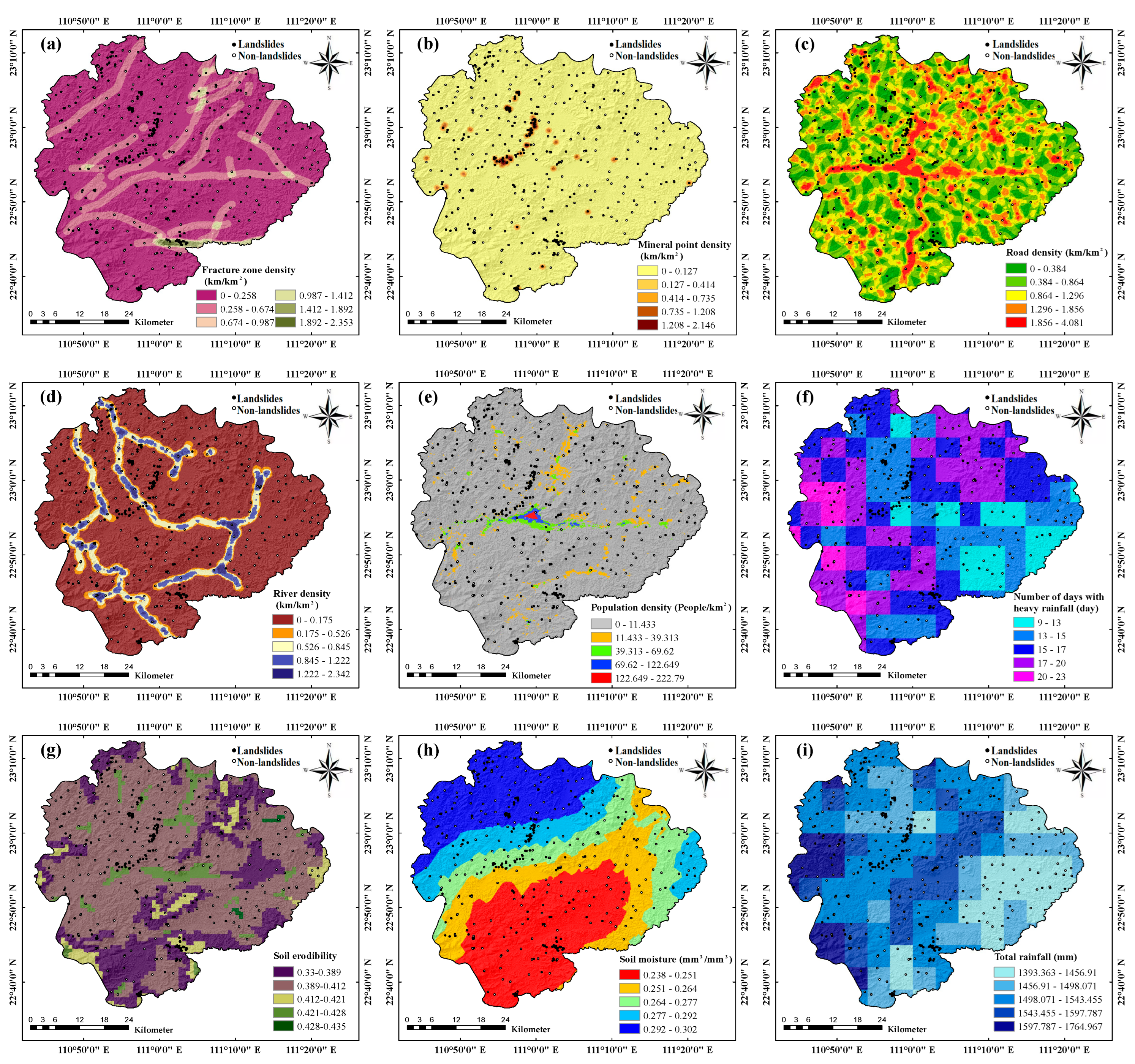
2.2. Data Acquisition

Having precise historical data on landslides is vital when examining and evaluating the potential for landslide catastrophes in a particular region [12]. The landslide inventory was created in this study using various methods such as Google Earth images, optical satellite images, and disaster news reports. Multiple data sources were utilized in this study to construct an inventory of historical landslides. First, the approximate locations where historical landslides occurred were identified through visual interpretation with the help of Google Earth software. Then, the location and extent of these landslides were further confirmed using optical remote sensing imagery, specifically, optical satellite imagery. These images provided high-resolution surface information that enabled more accurate identification and definition of landslide areas. In addition, disaster news reports and relevant literature were reviewed to obtain detailed information on historical landslide events, including the exact time, location, and number of occurrences. A total of 214 historical landslide areas were ultimately collected, providing essential data for interpreting the characteristics of landslides in the region and predicting their occurrence.
Landslide occurrences are typically the result of a combination of internal geological and topographic conditions within the slope and external environmental factors [35,36,37]. Therefore, the importance of choosing precise and suitable modeling data cannot be overstated when utilizing machine learning (ML) techniques to forecast landslide susceptibility. In this research, the conditions for the development of landslides in Cenxi were studied, which involved analyzing the geological and environmental information and the distribution status of historical landslides. The research area encompassed various aspects, including geological and soil information, topography, meteorological and hydrological conditions, land cover, soil conditions, and human activities, for a total of 23 factors selected to study the susceptibility to landslides. Table 1 provides the origins and explanations of these conditioning factors that contribute to landslides. Due to variations in coordinate systems and resolutions among different factors, the ArcGIS 10.2 software was used to project all factor data onto the UTM-Zone48 coordinate area based on the WGS1984 reference surface. All factors were transformed to a uniform spatial resolution of 30 m by generating a target raster using the Shuttle Radar Topography Mission (SRTM) data with a resolution of 30 m by 30 m.

2.3. Construction of the Modeling Dataset

The majority of landslides in the area typically happen on a limited scale, with the size of the slope altering before and after the occurrence of the landslide. Therefore, the landslide sample used for modeling was taken from the center raster of the landslide surface [38,39]. In selecting the non-landslide samples used for landslide susceptibility modeling, the following principles were fully considered in this study to ensure the reasonableness and representativeness of the sample selection:
(1)
First, to avoid sampling in areas with similar geography to known landslides, areas beyond 100 m from historical landslides were chosen as the selection range. This helped to maintain sample diversity and avoid introducing unnecessary bias due to geographic similarities.
(2)
Second, land areas that do not contain permanent bodies of water were extracted as the area for non-landslide samples. The consideration behind this principle is that landslide events do not usually involve areas of water bodies, ensuring that non-landslide samples were carefully selected; with an emphasis on this aspect, the selected samples were more geographically and geomorphologically similar to landslide events.
(3)
Given that landslides typically occur on steep slopes possessing higher slope values, areas with slopes less than 30° were extracted as extraction areas for the non-landslide samples. This selection helps to maintain similarity to landslide events, as steep-slope areas are more prone to landslides. Through this principle, we pursued maintaining a reasonable match of geomorphic features in the sample selection process.
Based on the above principles, criteria for selecting non-landslide sample areas were delineated. A total of 214 non-landslide samples were selected at random, maintaining a ratio of 1:1 with the number of landslide samples. This ratio was chosen to help keep the samples balanced and to allow the modeling dataset to contain a sufficient quantity of positive and negative samples. A total of 428 samples were created by merging the chosen landslide samples (labeled as 1) with the non-landslide samples (labeled as 0) for modeling purposes. Eventually, the dataset containing all the relevant data was randomly split into a training set with 299 samples and a test set with 129 samples, maintaining a ratio of 7:3. The dispersion of sample points in the landslide moderator layer as shown in Figure 2a–i, Figure 3a–i, Figure 4a–e.

3. Methods

The main objective of this research is to examine how various types of factor data affect the accuracy of landslide susceptibility models that rely on an ensemble machine learning framework. Additionally, the methodology of interpretability using SHAP is used to explain the influence of factors on data types, both globally and locally, in landslide susceptibility models to influence the decision mechanism of predictive results. The data processing platform used in this study is ArcGIS 10.2, and the programming language utilized is Python. The research procedure encompasses the subsequent stages, as outlined in Figure 5.
(1)
The process involves preparing data and constructing a spatial database that includes both samples from landslides and non-landslides, as well as conditioning factors that contribute to landslides.
(2)
Independence testing of landslide conditioning factors, including Pearson correlation analysis and multicollinearity diagnosis, is performed.
(3)
Preparation of the modeling dataset. In order to partition and standardize the attribute intervals of each factor, five different conditional probability models were employed: frequency ratio, statistical index, certainty factor, evidential belief function, and weights of evidence. Afterward, the data of the initial and processed factors were extracted to the sample points, resulting in the creation of six modeling datasets.
(4)
Landslide susceptibility modeling. Based on the six different modeling datasets, twelve landslide susceptibility prediction models were constructed using the random forest and extreme gradient boosting algorithms, and landslide susceptibility maps were generated.
(5)
Evaluation of model predictive performance. The performance of the twelve models as compared and analyzed using different statistical methods, identifying the best-performing model.
(6)
Shapley Additive exPlanations (SHAP) analysis. The influence of every factor on the models was investigated through the creation of SHAP models for all twelve landslide susceptibility models and the dependency relationship between the predictive results and features in models built using different machine learning methods and types of factor data.

3.1. Analysis of Conditioning Factors

Since landslides occur due to the combined effect of multiple adjustment factors, the diversity and complexity of the factors need to be fully considered [40]. Based on historical studies and expert experience, there may be statistical covariance among the initially selected landslide adjustment factors, which can lead to the inability of the landslide susceptibility model to accurately analyze the proper relationship between the evaluated factors and landslides [41].
Conducting a correlation analysis on the 29 identified moderating factors is necessary due to potential correlations among the indicator factors that may impact the accuracy of the landslide susceptibility model. The aim of this paper is to utilize the Pearson correlation coefficient (PCC) to evaluate the correlation between the layers of the factor. The calculation formula is described as Equation (1). A weak correlation between the factors is indicated if the PCC value is less than 0.6, and the opposite is also true. There is a significant correlation [42]. In addition, to ensure the independence of the data when building a multiple regression model, the degree of multivariate co-linearity of each factor was measured by calculating the tolerance (TOL) and variance inflation factor (VIF). Severe multicollinearity is indicated when the VIF value for a factor exceeds ten or the TOL value is below 0.1 between the factor and other factors, and the factor should be removed from the model The calculation formula is:
P C C = i = 1 n x i x ¯ i = 1 n y i y ¯ i = 1 n x i x ¯ 2 i = 1 n y i y ¯ 2
V I F = 1 T O L = 1 1 R 2
where  x i  and  y i  denote the    i -th variable between factor  x  and factor  y x ¯  and  y ¯  are the means of all variables in factor  x  and factor  y , respectively, and  n  is the number of variables in the factor; the coefficient of determination  R 2  is utilized to measure how well the independent variable explains the variation in the dependent variable in regression analysis. Additionally,   TOL  and  VIF  are reciprocally related to each other.

3.2. Conditional Probability Models

When evaluating landslide susceptibility, the factors evaluated at all levels are not only characterized by high data volume but also exhibit inconsistency in magnitude, which may lead to overfitting or underfitting after inputting into the model. To avoid this effect, the conditional probability model can subdivide and standardize each factor to establish a preliminary link in the interaction between landslides and the factors that moderate them. The connection between the pre-existing probability of landslides for each factor under evaluation and the probability of landslides occurring in various classification states is established based on historical landslide data [43,44]. Therefore, in this study, the frequency ratio, statistical index, certainty factor, evidential belief function, and weights of evidence were selected to convert the initial data of landslide adjustment factors into values reflecting landslide susceptibility, and the ML model utilized the calculated results to generate maps indicating the susceptibility to landslides.

3.2.1. Frequency Ratio

The method of bivariate statistics known as the frequency ratio (FR) is straightforward. The likelihood of a landslide happening is calculated by the analytical model, which allows for a quantitative assessment of landslide susceptibility in different secondary classification intervals for each factor, combined with spatial data [45,46]. FR has been widely used in hazard probability assessment involving several geographic layers [47]. The formula for the calculation is as follows:
F R i j = N i j N S i j S
where  F R i j  is the frequency ratio of the  j -th secondary classification level of the  i -th moderating factor.  F R i j    > 1 means that the corresponding factor conditions are favorable for landslide occurrence;  F R i j    < 1 indicates that the attributes of the factor interval are weakly related to landslide occurrence;  F R i j    = 0 means that the factor  i  does not provide landslide development information in the state  j N i j  is the number of landslides occurring in the  j -th secondary classification interval of factor  i S i j  is the quantity of rasters in the interval;  N  is the number of landslides; and  S  is the number of rasters in the interval.

3.2.2. Information Value

The derivation of information value (IV) involved the creation of a blend of statistical models and information theory. The assessment of geohazard susceptibility is performed using a statistical method that relies on informative values. This method transforms the distribution of landslides across various factors in the study area into quantifiable magnitudes that provide valuable information. By examining the amount and level of detail in the data pertaining to regions affected by landslides, we can determine the likelihood of landslides occurring in the research region. The formula for the calculation is as follows:
I V i j = ln D i j D = ln   N i j S i j N S
where  I V i j  represents the quantity of information at the  j -th level of secondary classification for the  i -th adjustment factor;  D i j  is the landslide density in the  j -th secondary classification interval of the  i -th adjustment factor; and  D  is the landslide density in the whole area. The parameters of  N i j S i j N , and  S  are the same as those in Section 3.2.1.

3.2.3. Certainty Factor

In 1975, Shortliffe and Buchanan proposed a segmented probability function called the Certainty Factor (CF). In 1986, the model was further improved by Heckerman to analytically study the sensitivity of factors affecting the occurrence of an event. The statistical relationship is believed to determine the probability of landslide occurrence between known landslides and adjustment factors [48]. The representation is as follows:
C F i j = P P i j P P s P P s 1 P P i j   P P i j < P P s P P i j P P s P P i j 1 P P s   P P i j P P s
where  C F i j  indicates the certainty coefficient of landslide occurrence in the  j -th secondary classification interval of the  i -th factor and takes values in the range of [–1, 1]. When CF > 0, a more significant value indicates a higher probability of landslide; when CF < 0, a smaller value indicates a lower probability of landslide; when CF = 0, it is impossible to judge whether a landslide will occur.   P P s  is the a priori probability of landslides occurring in the entire study area, expressed as the ratio of the total number of landslides in the whole study area to the total number of rasters in the study area.  P P i j  is the conditional probability of landslides occurring in the  j -th secondary classification interval of the  i -th adjustment factor, which is usually expressed as the ratio between the number of landslides and the number of rasters in the factor classification used for the study.

3.2.4. Evidential Belief Function

The Evidential belief function (EBF) is a model that incorporates spatial integration and is rooted in the theory of the Dempster–Shafer evidence algorithm [49]. The EBF method has been widely adopted in numerous research domains and has yielded favorable outcomes when investigating susceptibility to landslides [50]. EBF has the benefit of being able to effectively process diverse incomplete data, resulting in outputs that specifically reflect belief (Bel), disbelief (Dis), uncertainty (Unc), and plausibility (Pls). There are four parameters that comprise the EBF model, which are calculated by the following equations:
W E i j = N L E i j N L N E i j N L E i j N A N L
B e l i j = W E i j j = 1 m W E i j
W ¯ E i j = N L N L E i j N L N A N L N E i j + N L E i j N A N L
D i s i j = W ¯ E i j j = 1 m W ¯ E i j
U n c i j = 1 D i s i j B e l i j
P l s i j = 1 D i s i j
where  B e l i j  is the degree of belief;  D i s i j  is the degree of disbelief;  Unc ij  is the degree of uncertainty; and  P l s i j  is the degree of plausibility. The range of values is [0, 1].  N L E i j  and    N E i j  are the number of landslides and the number of rasters in the  j -th secondary classification interval of the  i -th factor, and  N L  and  N A  are the number of landslides and the number of rasters in the whole region, respectively. In this study,  Bel  was used as a factor importance evaluation index. A higher  Bel  indicates a higher probability of landslide occurrence, while a decrease in  Bel  indicates a decrease in the likelihood of landslides occurring, and when  Bel  is 0, it means that no landslide data are available to prove the probability of landslide occurrence.

3.2.5. Weights of Evidence

An event’s likelihood of happening by combining different pieces of evidence can be estimated using the weights of evidence (WOE) approach, which is a quantitative method that employs a Bayesian criterion. It has been widely used by many scholars for multivariate information synthesis and spatial decision support systems [51,52]. Nowadays, many scholars use this model to assign weights to each landslide moderator to evaluate and analyze the landslide susceptibility of a district [51,53]. The weights, both positive and negative, along with the final combined weight, are calculated as follows:
W i j + = ln P B D P B D ¯
W i j = ln P B ¯ D P B ¯ D ¯
C i j = W i j + W i j
In the equation,  P B D  and  P B D ¯  represent the probabilities of landslide occurrence and non-occurrence, respectively, under the secondary classification level of a regulating factor;  P B ¯ D  and  P B ¯ D ¯  represent the probabilities of landslide occurrence and non-occurrence, respectively, in areas except for the secondary classification level of a regulating factor; within the second-level classification of this factor,  B  and  D  denote the count of landslides and non-landslides, respectively, and, except for the second-level classification of this factor,  B ¯  and  D ¯  correspond to the count of landslides and non-landslides;  C i j  stands for comprehensive weight, the weight of the  j -th secondary classification interval of the  i -th factor to the landslide. The larger the value of  C i j , the more indicative the secondary classification level of the factor is of the probability of landslide occurrence. If  C i j    = 0, it means that the secondary classification level of the factor does not indicate landslide occurrence;  C i j    > 0 indicates a favorable condition for landslide occurrence; and  C i j    < 0 indicates an unfavorable condition for landslide occurrence.

3.3. Tree-Based Machine Learning Models

3.3.1. Random Forest

An algorithm called random forest (RF) was proposed by Breiman to integrate multiple decision trees. It mainly extracts a plurality of samples from the initial dataset and proceeds to train these gathered samples using the decision tree algorithm, then derives the ultimate prediction outcome based on the combined decision tree results through a voting process [30]. The RF algorithm finds its utility in both classification and regression tasks. In contrast to conventional machine learning techniques like artificial neural networks, logistic regression, and support vector machines, RF prevents model overfitting through random sample selection and exhibits a level of resilience towards outliers. In addition, it has high accuracy, facilitating comprehensive data examination of high-dimensional feature data [19]. This research applies the RF algorithm within the Python 3.9 environment using the ”sklearn. Encrypt” package.

3.3.2. Extreme Gradient Boosting

Chen T et al. introduced a technique called extreme gradient boosting (XGBoost) in 2016, representing a novel machine learning approach which can be used to scale up the tree boosting algorithm, a popular method for landslide susceptibility modeling prediction in recent years. Like RF, XGBoost is an integrated learner that uses decision trees as building blocks. However, unlike RF, XGBoost uses boosting in its integration learning process [54]. By utilizing weak decision trees as the foundational learner during training, it amalgamates preferences to produce a robust collective evaluator. The algorithm effectively prevents the occurrence of overfitting. It improves the model accuracy by improving the boosting algorithm by adding a regularization term when addressing the loss function’s extreme values. In addition, the convergence speed is faster and computational efficiency higher than other algorithms. The main practical function of XGBoost is shown in Equation (15). This research incorporates this technique within the Python 3.9 environment through utilization of the “XGBoost” Python package.
y ^ i t = k = 1 t f k x i = y ^ i t 1 + f k x i
where  y ^ i t  represents the sample’s predictive outcome  i  after the  t -th iteration;  y ^ i t 1  signifies the preceding predictive outcome of  t  − 1 trees;  f k x i  denotes the function associated with the  t -th tree.

3.4. Model Evaluation Criteria

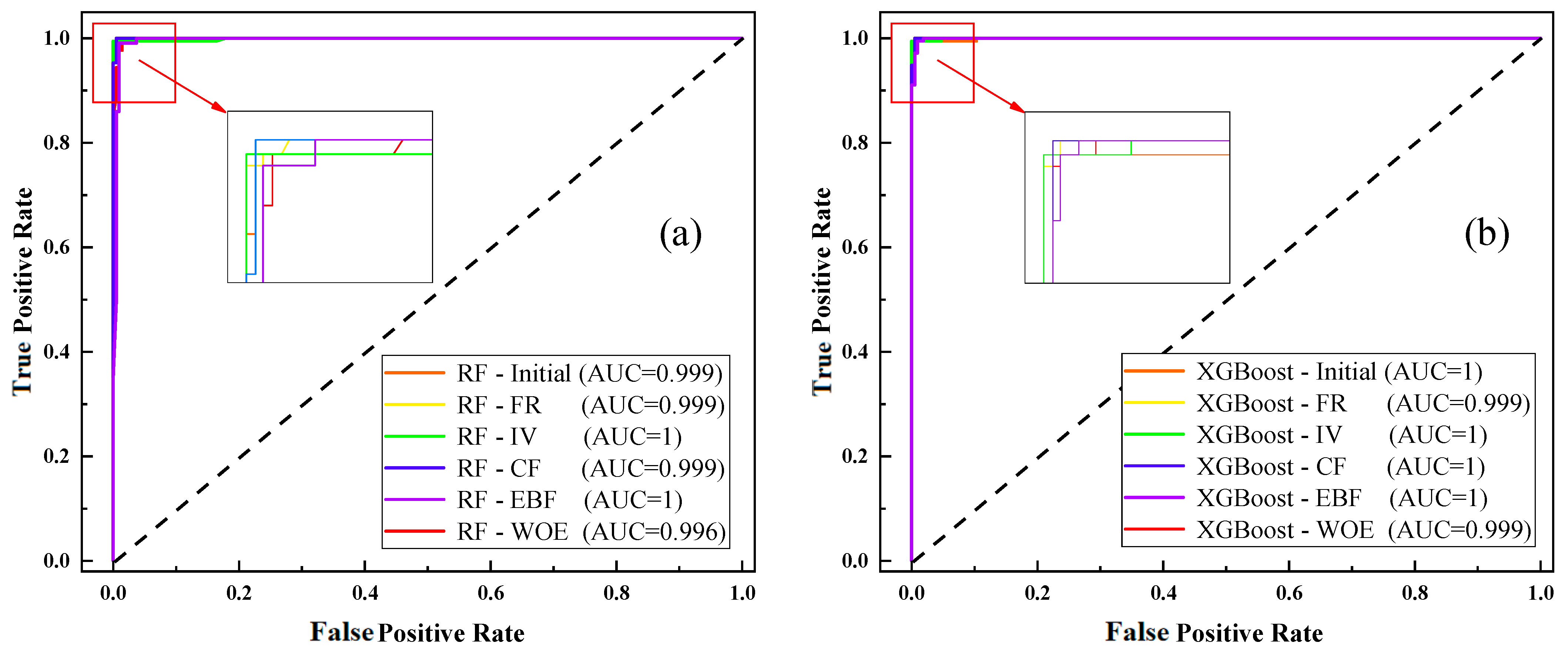
3.4.1. Receiver Operating Characteristic

The ROC curve is frequently utilized to assess the results of landslide susceptibility experiments in a qualitative manner [55]. The horizontal axis corresponds to the false positive rate (1-specificity), illustrating the accumulating percentage of terrain classified from high to low susceptibility. Meanwhile, the vertical axis signifies the true positive rate (sensitivity), indicating the accumulating percentage of landslide samples. The AUC value reflects the probability of a randomly chosen positive sample outranking a randomly chosen negative sample, and the model’s effectiveness in accurately predicting landslide occurrence or absence is evaluated based on this metric [13]. In the case of AUC > 0.5, a higher AUC value signifies a superior model fit. The formula for the calculation is as follows:
A U C = T P + T N P + N
where TP represents the count of accurately predicted landslide samples; TN represents the count of correctly predicted non-landslide samples; P represents the total count of landslide samples; and N represents the total count of non-landslide samples.

3.4.2. Confusion Matrix

When assessing the accuracy performance of a binary classification model for landslide susceptibility, a confusion matrix is often used [56]. The true positive (TP) in the confusion matrix indicates the number of accurately predicted landslide samples, whereas the false negative (FN) signifies the quantity of incorrectly predicted landslide samples. Additionally, the term “true negative” (TN) is used to describe the count of correctly predicted samples that are not landslides. An incorrect prediction of non-landslide samples is what is known as a false positive (FP). Using five statistical indicators, this study evaluated the accuracy of the landslide susceptibility model in predicting future occurrences, including true positive rate (TPR), true negative rate (TNR), accuracy (ACC), F1 score (F1), and kappa coefficient (KC). In detail,  T P R  represents the proportion of correctly classified landslide samples;  T N R  represents the proportion of correctly classified samples that are not landslides;  A c c  represents the proportion of accurately classified samples in the entire set; and the  F 1  value is capable of offering a thorough evaluation of the model’s prediction performance for landslide samples. It quantitatively represents the degree of consistency between the predicted attributes of the samples and their actual attributes. The formula for the calculation is as follows:
T P R T r u e   P o s i t i v e   R a t e = T P T P + F N
T N R T r u e   N e g a t i v e   R a t e = T N F P + T N
A c c = T P + T N T P + F P + F N + T N
F 1 s c o r e = 2 T P 2 T P + F N + F P
K C = P 0 P e 1 P e where   P 0 = T P + T N T P + F N + F P + T N ,     P e = T P + F N T P + F P T N + F N F P + T N T P + F N + F P + T N 2

3.4.3. Root Mean Square Error between the Predicted and Actual Values of the Sample

To evaluate the precision of a model’s prediction, the commonly used approach is to utilize the root mean square error (RMSE). A smaller  R M S E  value signifies that the prediction results of the sample data are more closely aligned with the actual attributes, and the model performs better [56]. In this research, the RMSEs for predicting the overall, landslide, and non-landslide samples with their corresponding true values are calculated in this paper. The results are named RMSE, RMSE-1, and RMSE-0, respectively.
R M S E = 1 N i = 1 N Y i f X i 2
where  N  represents the number of samples within the specific category from which the calculation will be performed;  Y i  represents the true value of the  i -th sample; and  X i  is the predicted value of the  i -th sample after model operation.

3.5. Shapley Additive ExPlanations

Shapley Additive exPlanations (SHAP) was suggested by Lundberg and Lee in 2017 as a game theory-based approach to interpret any machine learning model. In detail, the term “Shapley” pertains to the calculation of the Shapley value for every characteristic variable in the model, for each sample. The term “Additive” indicates that, for each sample, the Shapley value of every characteristic variable can be combined. The term “exPlanation” refers to the explanation of how each characteristic variable influences the predictive value of the model for each individual sample. The Shapley value of each feature illustrates its contribution to the final outcome forecast in order to explain the difference between the actual and average predicted values [57,58]. The interpretability of features is provided by SHAP both globally and locally and considers the interaction synergy between variables while considering the impact of individual variables. Given the excellent interpretability of SHAP for ML models, it has seen extensive use in interpreting disaster susceptibility and ecological environment domains [59]. The purpose of this research was to develop a landslide susceptibility model utilizing the RF and XGBoost algorithms, which was then interpreted and analyzed using the Shapley value estimation method from the SHAP theory of treeSHAP. The implementation of SHAP utilized the Python 3.9 library version 0.39.0 for SHAP. The SHAP value can be calculated. The formula for the calculation is as follows:
φ j x = S N \ j S ! N S 1 ! N !   f x S j f x S
where  φ j x  represents the SHAP value of the  j -th feature, indicating the effect of that feature on the sample  x N  is the total number of features;  S  is a subset of  N  with feature  j  removed;  f x S  represents the removal of features in  j  after removing the set of features  x S  corresponding to the model predictions;  f x S j  represents the model predictions corresponding to the feature set  x S j  after inclusion of feature  j S  denotes the size of the set  S ; and  N  denotes the total number of features.
The average of the SHAP values is designed to measure the overall impact of the features in the sample set on the model predictions. With the formula for calculation as follows, we can calculate the average of the SHAP value.
I j = 1 n k = 1 n φ j k
where  I j  represents the average SHAP value of the feature  j n  is the size of the sample set; and  φ j k  represents the SHAP value of the feature  j  in the sample  k .

4. Results

4.1. Landslide Conditioning Factors Analysis

In this paper, correlations between 23 landslide moderation factor layers were calculated using MATLAB R2022a software. After obtaining the correlation coefficients between the factors, we used the matplotlib.pyplot library in Python to visualize the correlation matrix. According to Figure 6, the positive correlation between the factors becomes stronger as the color gets lighter; the strength of the negative correlation between the factors increases as the color becomes darker. The results show that, among the 23 factors, the magnitude of the correlation coefficient between any pair of factors is below 0.6, indicating that the correlation between the evaluation factors is small. In addition, this paper used SPSS 20.0 software to analyze the factors for multicollinearity, and the results are shown in Table 2. All landslide adjustment factors had TOL values that were greater than 0.1; the VIF values were less than 10. Among them, the lowest TOL was 0.31, while the highest VIF was 3.24, indicating no multicollinearity among the factors. The combined analysis of the two indicators indicates that all factors satisfy the requirement of mutual independence and can be involved in landslide susceptibility modeling and evaluation [60].

4.2. Model Structuring and Optimization

Before constructing a landslide susceptibility model utilizing the ML method, the hyperparameters used for the different models need to be optimized [61]. After dividing the sample data randomly into training and test sets in the ratio of 7:3 (295:129), to improve the models’ ability to generalize, the training set was used to train the models with 10-fold cross-validation. Additionally, the hyperparameters were optimized using the grid search method [62]. The optimized hyperparameter values were also substituted into the model for training to construct a model for determining the likelihood of a landslide. Table 3 displays the explanations and names of the hyperparameters that will be modified in the RF and XGBoost models used in this research. Furthermore, the hyperparameters of different models that were optimized to obtain the optimal values using RF and XGBoost are listed in Table 4 and Table 5, respectively. The results showed that, based on the same modeling method, the hyperparameter values varied when modeling using different factor data types. Compared with the default parameters, when the optimized hyperparameters were employed, the model showcased enhanced accuracy in both training and validation.

4.3. Landslide Susceptibility Maps for Different Models

This study constructed 12 landslide susceptibility prediction models using two ML methods (RF and XGBoost) combined with six-factor data types (Initial, FR, IV, CF, EBF, and WOE), respectively. Then, the LSIs for all raster cells in the study area were estimated. The estimated values cover a range of values [0, 1]. Finally, to generate the corresponding LSMs, the LSIs of all raster cells in the study area were visualized using ArcGIS10.2 software. In order to compare and analyze the zoning results of different landslide susceptibility models, it is necessary to unify the classification thresholds of susceptibility classes. Therefore, this study classified the LSMs in the study area into five landslide susceptibility classes: very low, low, medium, high, and very high susceptibility. This classification was based on the fixed threshold method using intervals of [0,0.20], (0.20,0.50], (0.50,0.90], (0.90,0.95], and (0.95,1.0]. As a result, six LSMs using the RF model (see Figure 7) and six LSMs using the XGBoost model (see Figure 8) were obtained.
Overall, on the premise of the same factor data type, the LSI distributions obtained using the RF and XGBoost models predictions are approximately the same, with significant differences in details. In addition, LSMs generated using factor data processed by different conditional probability models based on the same ML model have a high similarity in the scattering of LSIs across the region. Compared with the LSMs generated using initial factor data, there are fewer high-susceptibility areas, eliminating the spatially discontinuous anomalous areas and effectively improving the reasonableness of the prediction results of landslide susceptibility.
In order to conduct a quantitative analysis of the distribution of landslides across various areas classified by their susceptibility levels, the statistical analysis tools in ArcGIS10.2 were used to calculate the area, the quantity, and the frequency ratio of landslides in areas of distinct susceptibility grades (see Table 6 and Table 7). The frequency ratios of all models are on the rise with an increase in the susceptibility level except the susceptibility level area with the frequency value of 0 (not statistically significant). Moreover, the frequency ratio exhibited by all models within the high-risk zone significantly surpasses that observed in the low-risk region. The LSMs generated in this study are all reasonable.
The main objective of evaluating regional landslide susceptibility prediction outcomes is to identify and be alert about areas at risk of landslides [63]. Therefore, in this study, the “extremely high + high” susceptibility areas of different landslide susceptibility models is mapped as the landslide risk area (see Figure 9). The statistical results show that, based on the same factor data type, LSMs generated by XGBoost have marked more landslide risk areas and have more landslide samples. However, the mapping of RF to the landslide risk area is insignificant. For the XGBoost model, LSMs generated by different types of factor data have different responses to landslide risk areas. With the exception of the XGBoost-Initial model, the XGBoost-CF model, determined by the CF values of factor data, encompasses a landslide risk region that constitutes 24.959% of the entire study area, encompassing 91.121% of all landslide samples across the study area. The XGBoost-CF model completely contains both landslide risk areas and those pertinent to landslide samples and has good zoning results.

4.4. Model Accuracy Evaluation

The ROC curves express the correlation between the cumulative proportion of landslide occurrences and the landslide susceptibility index. They are used to evaluate the models’ overall performance and generalization ability. Figure 10 displays the ROC curves for the different models, which were derived from the testing set; Figure 11 displays the ROC curves of the various models when considering the entire sample set. Figure 11 displays the AUC values for the RF model and the XGBoost model on the testing set and the full sample set, considering different types of factor data. The AUC values of both the RF and XGBoost models for the testing set and the full sample set are nearly equal to 1. This implies that there is strong generalization ability among all models, and there is no occurrence of overfitting or underfitting. In addition, for the same type of factor data, the AUC values of the XGBoost model exhibited greater significance compared to those of the RF model, which proves the superiority of the XGBoost model again.
In this study, the prediction accuracy and feasibility of different landslide susceptibility models were evaluated based on the confusion matrix and sensitivity, specificity, accuracy, F1 score, and kappa coefficient with the premise of validating the overall performance of the models. The accuracy evaluation of distinct RF models and XGBoost models, based on the complete sample dataset, is depicted in Table 8 and Table 9, respectively. Overall, all models can provide an accurate representation of the landslide susceptibility in the study area. The maximum number of prediction errors for landslide samples is two; a maximum of five predictions can be made for non-landslide samples. In general, models built with XGBoost had higher prediction accuracy than RF models when using the same type of factor data for the samples. In addition, the LSMs generated using factor data processed by different conditional probability models have higher prediction accuracy than the initial factor data. Among them, RF-EBF and XGBoost-EBF models constructed based on EBF data for factors had the highest prediction performance. They have improved TPR by 0.467, TNR by 1.869, accuracy by 1.168, F1 score by 0.012, and kappa coefficient value by 0.023 compared to the RF-Initial and XGBoost-Initial models. The XGBoost-CF model and XGBoost-FR model each had a prediction error number of one for landslide and non-landslide samples, and the prediction performance of landslide susceptibility ranked second.
The reliability of the model is crucial in the work of predicting landslide susceptibility. Suppose we only pay attention to the model’s prediction accuracy and disregard its reliability and stability. Under these circumstances, the landslide susceptibility model will lose substantial application significance [64]. Therefore, this study examined the model’s reliability and stability in addition to assessing its prediction performance. Figure 12 and Figure 13 show the analysis of the scatter of target and output values of the sample data set based on different types of data types for the RF and XGBoost models, respectively. The RMSE values for the XGBoost model were lower than those for the RF model, including RMSE, RMSE-1, and RMSE-0, when using the same factor data, which were more stable and reliable models. Among them, the RMSE values were reduced by 0.0151–0.0305, RMSE-1 by 0.0077–0.0276, and RMSE-0 by 0.0163–0.0367.
In addition, the landslide susceptibility model built using the factor data obtained after conditional probability model processing exhibits a reduced RMSE for predictive reliability compared to the initial factor data for the same machine learning model. The RMSE values were reduced by 0.0074–0.0185 for the RF models except for RF-WOE. For the XGBoost models, the RMSE values were decreased by 0.0117–0.0186 except for XGBoost-WOE. The WOE model did not improve the performance of the other conditional probability models. The reason that the WOE model did not improve the model performance as much as other conditional probability models was that the weights of evidence for the secondary classification of the factors depended on the number of pixels of the landslides during the modeling process, and the method overestimates or underestimates the weights if the second level of classification for a factor is minimal and the landslides are not evenly distributed. Accordingly, instead of calculating the area of each landslide, the number of spaces where landslides occur was chosen as a modeling sample in this paper. Therefore, it is inevitable that the WOE model does not enhance or even reduce the performance of the landslide susceptibility prediction model in this study. From a comprehensive analysis, the above findings demonstrate that selecting a suitable conditional probability model has an essential influence on developing stable and reliable landslide susceptibility models. Moreover, among the 12 models, the XGBoost-CF model has the lowest RMSE value (RMSE = 0.0807, RMSE-1 = 0.0929, RMSE-0 = 0.0663) and the highest stability and reliability.
In summary, the XGBoost model effectively enhances the prediction performance of landslides compared with the RF model. Among them, the XGBoost-CF model stands out as an effective solution for enhancing the accuracy of predictions made by the model while ensuring the reasonableness of landslide susceptibility zoning results and has the highest stability and reliability among all models. Therefore, the XGBoost-CF model outperforms the other 11 models in this study, making it the most optimal choice.

4.5. Shapley Additive ExPlanations (SHAP) Analysis

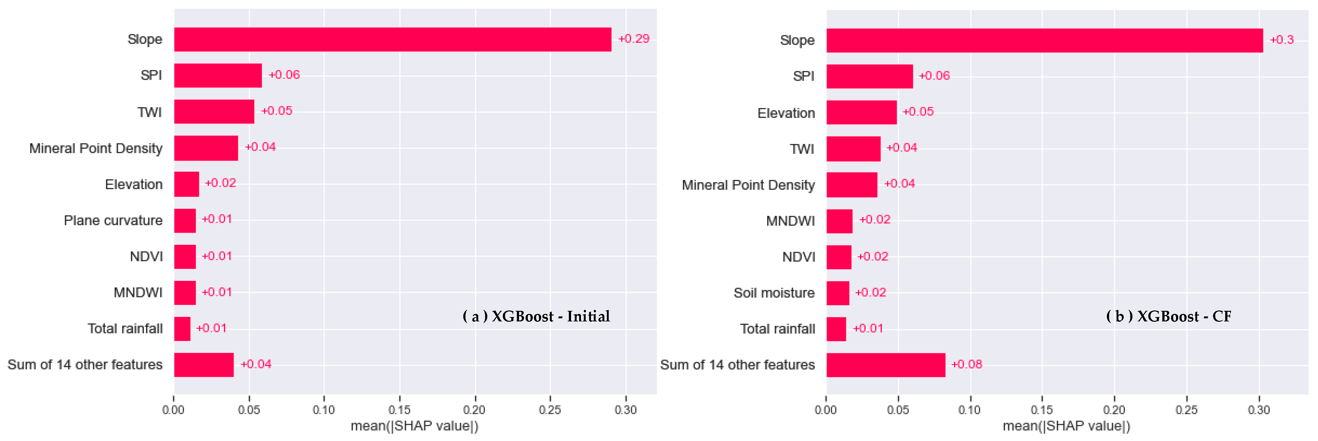
4.5.1. Factor Importance Based on Shapley Value

To obtain a general understanding of which adjustment factors hold the greatest significance in relation to the landslide susceptibility model, this study uses the “summary_plot” function to draw the Shapley value of each adjustment factor for each sample, which shows which factors have the most critical influence on the landslide and their influence range on the data set. As shown in Figure 14 and Figure 15, four landslide susceptibility models based on both Initial and CF types of factor data and using RF and XGBoost rank the factors according to the sum of Shapley values of all sample data and use Shapley values to show the influence distribution of each factor on the model output. The points in the figure represent the sample data, and the color indicates whether the factor value of each sample is high or low (red: high, blue: low). The color enables us to match how the change in factor eigenvalue affects the change in landslide susceptibility. The position on the horizontal axis is determined by each Shapley value. However, the overlapping points fluctuate in the vertical axis direction so that we can know the Shapley value distribution of each factor, and their importance sorts these features.
The outcomes showed that there was both uniformity and variability in the distribution and ranking of Shapley values across various landslide susceptibility models. The uniformity is demonstrated by the fact that slope, SPI, TWI, mineral point density, and elevation are all rated as the most influential factors in the different models. Among them, the slope has the highest Shapley value due to its extensive extension in the horizontal axis direction, so it is considered the factor with the highest importance and interaction in landslide susceptibility prediction. As for the several factors ranked lower in the different summary plots of SHAP, although their Shapley values are lower, they also impact the prediction performance of the model and are indispensable for constructing excellent and comprehensive landslide susceptibility models.
The differences are mainly manifested in two aspects. Firstly, although different models have good performance in predicting landslides, the chosen models could improve the consistency of their decision-making mechanisms, causing variations in the distribution of Shapley values for the same factor across different models. Secondly, when founded on the initial factor data, the positive and negative correlations of different factors on landslide susceptibility prediction are different in the model. On the contrary, in the model constructed using the factor data obtained after the conditional probability model, almost all factors positively correlate with landslide prediction. For example, when using the initial data of factors, continuous factors such as TWI, NDVI, MNDWI, road density, and plane curvature and discrete factors such as hydrogeology and the occurrence of landslides are more favorable when the factor value is lower, indicating a negative correlation with soil type. However, the data processed by conditional probability models such as FR, IV, and CF positively correlate with landslide prediction. This is because the conditional probability model based on statistical thought can standardize the factors with landslide data, as when the factor value increases, the risk of landslide also increases. On the premise of improving the prediction accuracy, the significant influence of factors on landslide prediction can be expressed more clearly, and the interpretability of the model to factors and their data can be increased.
The above analysis results show that the integrity of landslide adjustment factors, the data types of factors, and the prediction performance of the landslide susceptibility model will be greatly influenced by the modeling methods.
The average of the absolute Shapley values for each sample in Figure 14 and Figure 15 was computed in order to determine the individual significance of each feature in predicting landslides, and the factor importance was plotted using the “shap.plots.bar” function (Figure 16 and Figure 17). The outcomes showed that the contribution and importance ranking of the main factors affecting landslide prediction (top nine) varied among the different landslide susceptibility models. However, among all the models, the five factors of slope, SPI, TWI, mineral point density, and elevation are in the top five positions and make the main contribution to the accurate prediction of landslides. The sum of average SHAP absolute values of the following 14 factors are in the range of [0.04, 0.12], which have less influence on landslide prediction. Secondly, compared to the RF model, the XGBoost model highlights the pronounced impact of the slope factor more.

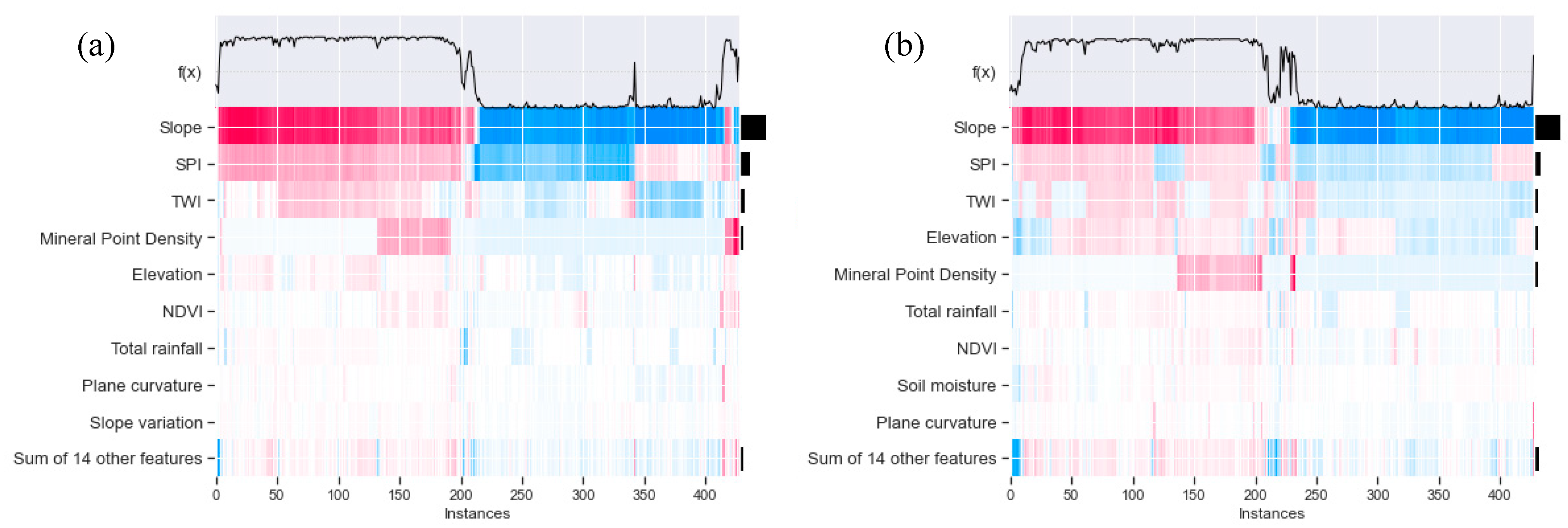
4.5.2. Influence of Factors on Prediction Result

In order to systematically display the overall results of the sample data set in the model and the influence degree of the main features on the predicted values of the samples, the Shapley value matrix is transferred to the “Shapley. Plots. Heat Map” function, and the heat maps of the RF model and XGBoost model based on different types of factor data are drawn by this function (Figure 18 and Figure 19). In the figure, the X axis is each sample, the ranking of samples is based on the hierarchical clustering method, and the samples are clustered by Shapley value. The Y axis is the influence of each factor on the sample. The color describes the impact of the factor on the sample. Above the color matrix is a curve formed by connecting the output values of the model. The bar chart on the right shows the global importance of each factor in the model.
According to the analysis, the heatmap can clearly show how the landslide adjustment factors generate the predicted value of each sample through the stacking of factors. It also shows the direction and strength of a factors’ influence on predicting landslide susceptibility, which achieves the interpretability and transparency of the model. In addition, for the same type of factor data, the heatmap’s prediction curves indicate that the XGBoost model produces highly smooth prediction results, while the RF model’s prediction results show relatively low smoothness. Among them, the XGBoost-CF model stands out among the others with its smooth prediction curve, as well as achieving the highest levels of prediction accuracy and stability. The findings of this research align with the analysis findings presented in Section 4.4, which again proves the superiority of the XGBoost-CF model.

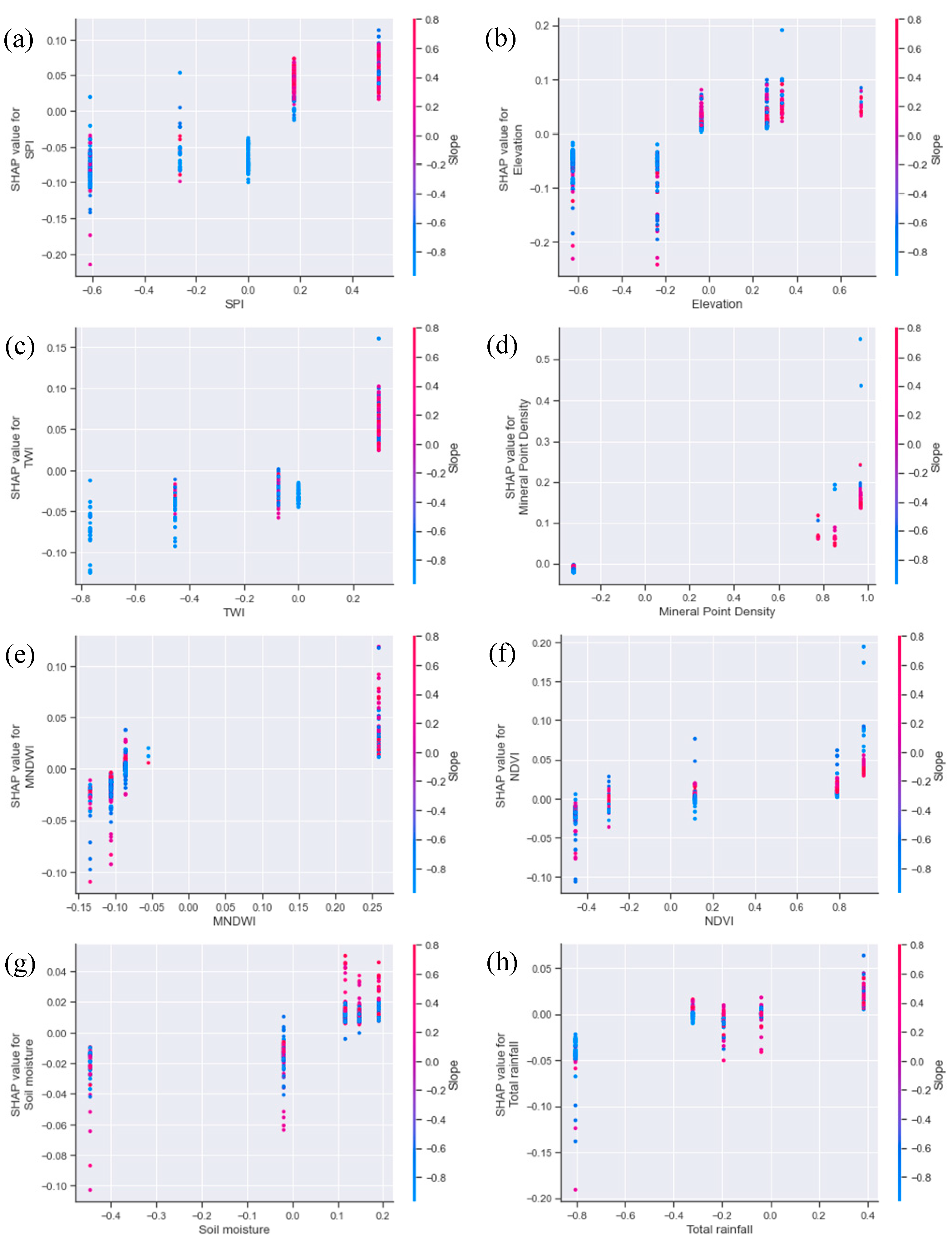
4.5.3. Dependence and Interaction of Factors

Dependence plots show the marginal effect of one or two features on the predicted outcome of a landslide susceptibility model, and they can show whether the relationship between landslide moderators and predicted values is monotonic, non-monotonic, or more complex. Dependency plots of factors fall into two categories. One describes how a single factor affects the predicted outcome of landslide susceptibility across the entire dataset. The other describes the effect of variables from two factors on the predicted development under interaction [36,65].
Examples of models used in this study include XGBoost-Initial and XGBoost-CF, based on different types of factor data from the whole modeling dataset. The function “shap.dependence_plot” is utilized for plotting single-factor dependence plots and analyzing the impact of the primary influential factors in each model on the prediction outcomes. Every variable in the dataset is represented by a point on the dependence plot; the value of a specific factor in the dataset is plotted on the horizontal axis, while the Shapley value for each sample of that feature is plotted on the vertical axis. The Shapley value indicates the extent to which that feature influences the prediction outcomes of the model. Figure 20 shows the factor dependence plots of the top nine most important factors in the XGBoost-Initial model. Different factors have different relationships with the prediction results across the entire dataset. Firstly, taking the slope factor as an example, the slope and the prediction results are monotonic. When the slope is less than 10 or more than 20, the increase in slope does not obviously result in an increase in the probability of a landslide, which shows that this range is conducive to landslide detection. However, when the slope is in the range of [8,18], the model is insensitive to detecting landslides, and most of the prediction errors are in this range. Among them, when the slope is greater than 18, the occurrence of landslides benefits from a Shapley value that is greater than 0. Secondly, SPI is not monotonic with the predicted results, and Shapley’s value changes sharply with the increase in SPI value. If the SPI value falls between 2 and 6, the Shapley value will be greater than 0 and the landslide risk will be elevated. Finally, the total rainfall is monotonic with the predicted results. If the total rainfall exceeds 1500 mm, then the Shapley value will be greater than 0, and landslide risk will be increased. The above analysis results of individual factors are in high agreement with the objective characteristics of landslides in this study area. Therefore, the dependence plots of a single factor based on the initial data can clearly show the complexity between factors and landslides and the interval and sensitivity of factors that affect the occurrence of landslides.
The dependence plot of the top nine factors in the importance ranking in the XGBoost-CF model is shown in Figure 21. Compared with the XGBoost-Initial model, the most obvious difference is that the scattering of the sample Shapley values does not have interval continuity; the scale value of the sample present on the horizontal axis is equal to the CF value of each secondary classification interval of the factor, and for the same factor data, the Shapley values of the samples of the secondary classification are scattered vertically along the vertical axis. The factor scatter’s Shapley value increases as the CF value of the factor increases, showing a positive relationship with the prediction results.
According to the dependence relationship between the factors based on CF value and the outcome of the prediction, the inconsistency between the influence degree of the factors obtained by SHAP and the statistical results calculated by the CF model can be observed. For example, as the factor CF value increases, the dispersion interval of the Shapley value for the slope factor also increases. Additionally, when the CF value of the slope is greater than 0, all the Shapley values of the samples are greater than 0. Thus, the factor positively affects landslides. However, in the case where the slope’s CF value equals −0.622, the Shapley value of certain samples exceeds 0, contradicting the statistical significance of the CF model. Likewise, when the CF value for the elevation factor surpasses 0, the Shapley values of all samples are greater than 0 as well. However, when the CF value is −0.034, it implies that the Shapley value of the samples in the secondary classification range of the corresponding factor is positive, indicating that the factor also encourages the occurrence of landslides.
The statistical significance of the CF model will not be fully considered when using the XGBoost algorithm combined with the CF data of the factors for landslide susceptibility prediction. Instead, the optimization aims to enhance the prediction performance of the sample by optimizing the degree of influence of the CF values on the prediction results in a global manner. Therefore, a priori statistical results of the influence of the factors on landslides obtained using the conditional probability model and the impact of the factors on the predicted results obtained using the ML method possess a notable discrepancy. The coupled model is beyond the capabilities of a basic superposition calculation to analyze.
From the analysis results of the single-factor dependence of XGBoost-Initial and XGBoost-CF models, the influence of individual factors on landslide susceptibility prediction results can be more comprehensively explained by considering both the initial data of factors and the factor data processed by the conditional probability model, taking into account their characteristics together. It is evident that this approach yields a clearer understanding of the prediction of landslide susceptibility.
Landslide phenomena arise from the combined effect of various factors. Therefore, it is important to investigate the relationship of how a factor interacts with another factor to influence the prediction results of landslide susceptibility once the extent of influence of a single factor regarding the outcome forecast has been analyzed. Figure 22 shows the double-dependence plot of the slope factor with the remaining main influencing factors in the XGBoost-Initial model.
The points in the figure indicate the Shapley values for every factor in all samples. Except for slope, the horizontal coordinates represent the range of values for the factors that exert the greatest impact on landslides. The vertical coordinates indicate the corresponding Shapley values for each sample. The color analyzes the distribution of the slope factor in the process of other factor changes. Throughout the dataset, landslide-prone samples with higher slope values are overwhelmingly samples with larger Shapley values in the other factors. This suggests a strong positive interaction between slope and other factors that can promote landslides. For example, for areas with SPI values at [2,6], the presence of larger slope values and Shapley values greater than 0 in the samples indicates a higher likelihood of landslides. Most sample points have larger slope values in the region where mineral point density is greater than 0, contributing to landslides. When the amount of rainfall surpasses 1500 mm, the majority of samples showing positive Shapley values tend to be found in regions characterized by steeper slopes. This demonstrates that the occurrence of landslides can either be enhanced or inhibited by the interaction between the factors and slope, which confirms that slope is the main influence of landslides in the region.
Based on Figure 23, in the XGBoost-CF model, if a factor’s CF value is above 0, the CF value of the slope for the sample, which has a Shapley value greater than 0, tends to be significant rather than being 0. It can be seen that slope and other main influencing factors also have a positive mutual effect with landslide prediction. As with the single dependence of the XGBoost-CF model, the horizontal axis is not sorted by the order of the classification intervals but by the CF values corresponding to the different classification intervals of the factors from smallest to largest. After analysis, as the CF values of the main factors affecting the slope increase, the number of samples with CF values greater than 0 for the slope gradually increases. The findings indicate that the mutual effect of the slope and each factor significantly affects the accuracy of prediction of landslide susceptibility. Moreover, the efficacy of the conditional probability model in improving the model’s performance is demonstrated.

5. Discussion

5.1. Features and Advantages of SHAP

When using the ML method to predict landslide susceptibility, the metrics can only account for a portion of the outcomes that the model forecasts, such as accuracy, precision rate, and recall rate. The model’s performance may fluctuate when various environmental factors change in the dimensions of time and space. Therefore, it is critical to understand how the model based on the ML method can make some decisions by modeling. To ensure the reliability, fairness, and transparency in the landslide susceptibility prediction model, the model’s explanation should include three aspects:
  • An understanding of whether each feature’s influence on the model’s final decision-making result is positive or negative along with the explanations for the respective influence.
  • An ability to find the feature interactions in the model and analyze how the interactions between features affect the prediction results of the landslide susceptibility model.
  • A local decision evaluation of the typical sample data in the model besides the global interpretation of the model.
The above is of great significance in explaining how the adjustment factors of the input model affect landslide susceptibility.
The traditional feature importance-ranking method can reflect the importance of each feature to landslide development locally and intuitively and illustrate which characteristics exert a considerable influence on the final model. Still, it cannot clearly show how the features affect the outcome of the forecast. One of the key benefits of the Shapley value is its ability to accurately represent the impact of each feature on every sample. It shows the positive and negative impact of features on the target. As shown in Figure 24, taking XGBoost-Initial and XGBoost-CF models as examples, the ranking results of landslide susceptibility importance obtained by using three characteristic importance calculation methods (weight, gain, and cover) attached to XGBoost are different and have significant differences. However, using the SHAP method based on Mean (|Tree SHAP|) can effectively avoid this phenomenon and has a high degree of attribution consistency (see Figure 25).
It can be seen that, given the complexity of the landslide phenomenon, there are unique advantages to analyzing the decision-making results of landslide susceptibility by using the SHAP interpretable method of ML model: (1) In addition to addressing the issue of multicollinearity, SHAP also takes into account the impact of individual variables and the combined effect of variables on the prediction outcomes. (2) SHAP not only contains more feature information than the traditional feature importance-ranking method but also fully ensures the consistency of global features and local samples.
It is important to note that this study exclusively utilizes SHAP to elucidate how various RF and XGBoost models, constructed with different types of factor data, generate predictions of landslide susceptibility. In doing so, it does not provide an objective explanation based on realistic principles. The RF and XGBoost models are developed using specific sample data, and thus any modification to the factors or samples may lead to alterations in the final decision regarding landslide susceptibility. Consequently, SHAP cannot be regarded as a straightforward causal model. To ensure that the explanatory results of the landslide susceptibility model closely align with objective reality, it is crucial to select a model with outstanding performance and ensure the accuracy of the sample data as well as the completeness of the adjustment factors.

5.2. Local Interpretation of Typical Samples

SHAP can explain the landslide prediction by landslide adjustment factors in the global dimension and analyze the influence of different factors in a single sample on landslide prediction to the local extent [40,41]. SHAP can visualize the contribution of factors to the n-th sample, find the explanation of the prediction results of a specific sample, and expose the model’s decision-making process for this sample. This study uses the local interpretation function of samples based on SHAP to analyze the contribution of factors to landslide and non-landslide samples. The study area utilized the RF-Initial, XGBoost-Initial, RF-CF, and XGBoost-CF models to interpret and analyze the locality of two representative landslide samples and two non-landslide samples.
For Case 1 (Figure 26), the predicted values of the four models are 1.00, 1.02, 1.00, and 1.00, respectively, and the prediction results of all models are more accurate and judged to be landslides. Topographic factors such as slope, SPI, and elevation positively contribute to landslides, and their corresponding Shapley value sums are more significant than 0.4. Although total rainfall, MNDWI, and soil type also contribute positively to this landslide, the degree of contribution is more minor, and their Shapley values are all around 0.01. The analysis results are consistent with the objective facts.
For Case 2 (Figure 27), the four models made predictions with values of 1.00, 0.96, 0.99, and 1.00, respectively. The RF-CF and XGBoost-CF models were the most precise in assessing the occurrence of landslides. Alongside topographic factors like slope, SPI, elevation, and TWI, mineral point density also plays a notable role in causing landslides, as reflected by Shapley values of 0.1 and 0.15. Moreover, the lower vegetation cover (NDVI = 0.117) allows landslides to develop. The Shapley value was in the interval of [0.02, 0.05]. Thus, it can be seen that the human mining and engineering behavior disrupts the state of equilibrium of the original stresses within the slope’s rock formation, destabilizing the rock and soil and leading to the landslide phenomenon. Therefore, slope is the primary condition factor of this landslide, and mineral point density is the main trigger factor. The analysis results are consistent with the objective facts.
For the typical non-landslide Case 1 (Figure 28), the predicted values of the four models were 0.23, 0.18, 0.38, and 0.01, respectively, and the XGBoost-CF model has the most accurate judgment result, and the judgment result is non-landslide. Although slope positively impacts landslides, TWI, SPI, MNDWI, soil texture, and road density are not conducive to landslides. The projected outcomes align with the objective facts.
In the case of non-landslide Case 2 (as shown in Figure 29), the four models had prediction values of 0.74, 0.64, 0.17, and 0.00, respectively. It is worth noting that the RF-Initial and RF-CF models made incorrect predictions, indicating a landslide occurrence. The XGBoost-CF model had the most accurate judgment result, and the judgment result was non-landslide, which was consistent with the objective facts.
According to the results of the local interpretation of typical samples using four models, the XGBoost-CF model of landslide susceptibility has the best prediction performance. The role of the slope factor is always of utmost importance when predicting landslides on both a global and local scale. Its contribution to the model is significantly higher than that of other factors. Furthermore, when compared to the RF algorithm, the landslide susceptibility model built with the XGBoost algorithm demonstrates greater accuracy in predicting samples. Moreover, the interpretation of factors using XGBoost is more reasonable and aligns better with objective facts.

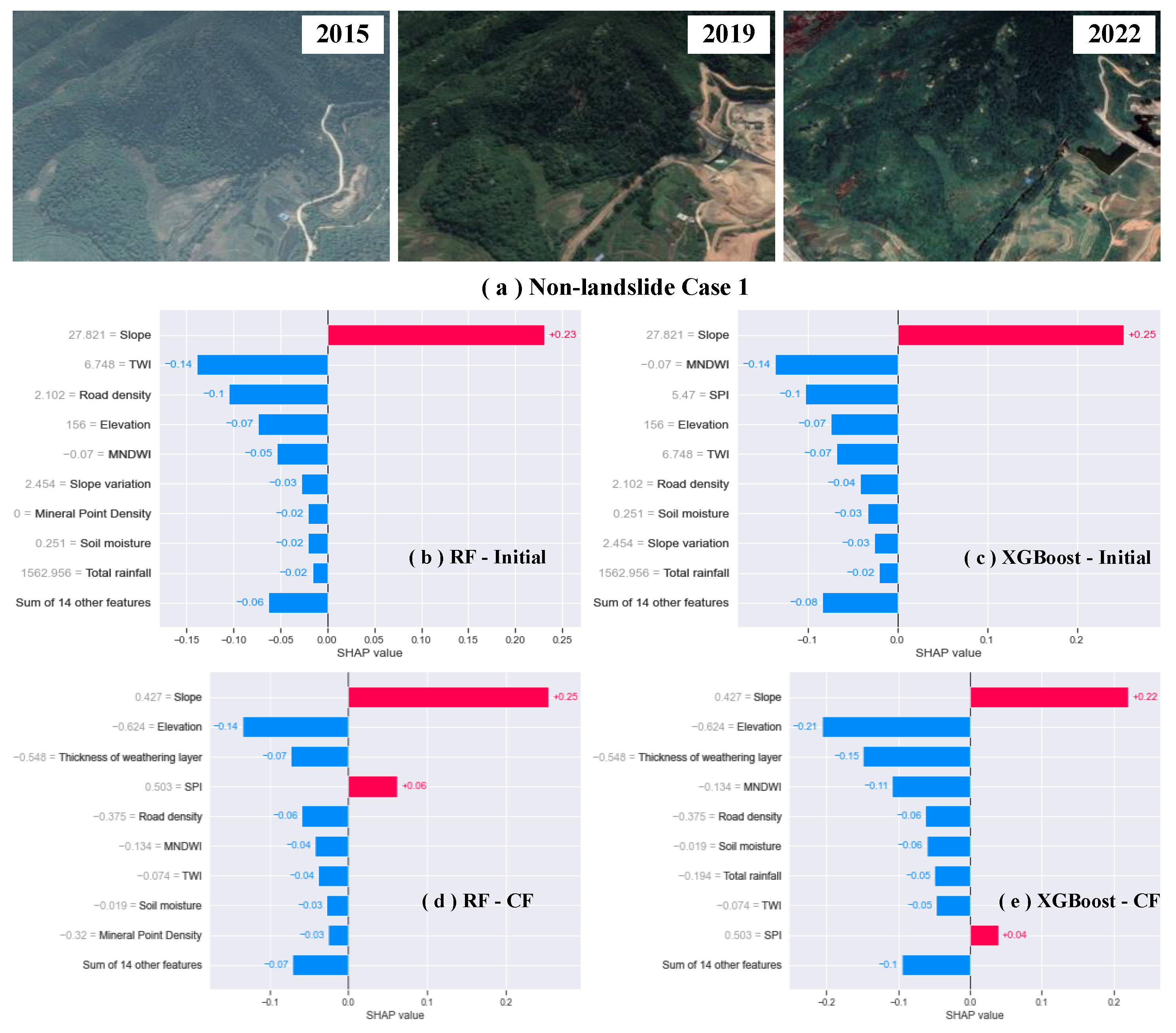
5.3. Local Interpretation of Samples with Wrong Prediction

The XGBoost-CF model exhibited the highest prediction performance in this study, with a single prediction error for both landslide and non-landslide samples. Therefore, to analyze the prediction errors of the models, this study provides a local interpretation and analysis of the samples with prediction errors in the XGBoost-CF model based on four models, RF-Initial, XGBoost-Initial, RF-CF, and XGBoost-CF, in the two dimensions of model and data type.
In Figure 30 and Figure 31, the images of the prediction error can see for both the landslide and non-landslide samples, as well as the local interpretation bar graphs, respectively. The Shapley value of each feature is represented on the horizontal axis. The vertical axis shows the factors that have the greatest influence on the prediction result of the sample, with the top factor being the most influential and the bottom factor being the least influential. The factor values of the sample are displayed on the left side. The color of the bar chart in the figure indicates the direction of influence of the factors on the prediction results, with red indicating a positive influence and blue indicating a negative influence. The length of the bars represents the degree of influence. Different models based on different decision mechanisms possess considerable differences in the interpretation of locality for the same samples. Figure 30a reveals a landslide sample with inaccurate prediction. The time series images clearly indicate that the sample exhibits evident signs of a landslide and falls into the category of a typical landslide sample. However, as seen in Figure 30b–e, the model mainly emphasizes the negative contribution of slope to landslide prediction. Compared with the positive effects of individual factors, the negative effects of slope, elevation, and other factors on landslide prediction are more significant, making the model output deviate from reality. We try to analyze the reasons for the prediction errors and conclude the following: Since the non-landslide samples in this study are mainly selected in areas with lower slopes, the number of samples with slope values less than 15° is as high as 197 out of 214 non-landslide samples, and the slope value of this landslide sample is 13.617°. Considering the conclusion that slope is the most influential factor in predicting landslides, this leads to an error in the model’s prediction of the given sample, classifying it incorrectly as a non-landslide.
On the other hand, for non-landslide samples with incorrect predictions in the XGBoost-CF model, as can be seen in Figure 31a, the surface environment of the area where the sample is located has remained unchanged in the time series and does not meet the conditions for landslide occurrence. It belongs to a typical non-landslide sample. From the output of the model, the RF-Initial and XGBoost-Initial models based on the initial data of the factor predict this sample as a non-landslide sample, and the prediction results are correct. Based on the factorial CF data, the RF-CF and XGBoost-CF models incorrectly predicted this sample as a landslide sample. Analysis of the local interpretation of the different models shows that, in the RF-Initial and XGBoost-Initial models, even though factors such as TWI may have a positive effect on the occurrence of landslides, they are far from being able to offset the significant negative impact of SPI and slope, ensuring the stability of the sample properties. However, in the RF-CF and XGBoost-CF models, the influence of slope on this sample changed from negative to positive, and the number of factors that positively influenced the occurrence of landslides became larger. The combined effect of all factors tends to predict the landslide of this sample positively, deviating from the actual properties of the sample, and the prediction result is a landslide. The reason for this phenomenon is that, when converting factor data using the certainty factor model, the interval and number of secondary classifications will determine the reasonableness and accuracy of the factor CF values, which will positively or negatively affect the model’s performance. For example, because the secondary slope classification in this study was not comprehensive enough, the non-landslide sample fell in the wrong interval. Hence, the influence of the slope factor on this sample was biased in both direction and strength, ultimately impacting the final decision of the model. However, when the model is built by utilizing the factor data processed by the conditional probability model, the secondary classification of factors is served for for landslide samples, which cannot consider the function of displaying the classification characteristics of complex non-landslide samples. Therefore, this kind of error is inevitable.
In summary, the landslide susceptibility model constructed by the XGBoost algorithm based on factorial CF data has excellent prediction performance. However, it also inevitably needs a better prediction for the sample data. After systematic analysis, to avoid the number of prediction errors to the maximum extent, the researcher improves the pre-processing process of data from two aspects: improving the rationality of non-landslide samples and the precision of the secondary classification status of factors.

5.4. Post-Programming

5.4.1. Exploration and Discussion

This paper specifically examines how the model’s internal decision-making process operates using the interpretable approach of SHAP. It is found that models constructed by different ML methods and factor data types have different decision-making mechanisms, and the same factor contributes to varying models with different directions, strengths, and interactions. The slope is the main factor that interacts with other factors to promote landslide occurrence. The proposed explainable landslide susceptibility model can explain the samples in local dimensions, which analyzes the causes of landslide occurrence and improves the prediction errors.
The research results in this paper further explore and apply the existing SHAP (Shapley Additive exPlanations) methodology, which adds significant value to the explanatory analysis of modeling susceptibility to landslides. The following is a discussion of how the research results of this paper complement, confirm, or contradict the current state of SHAP research:
  • Exploration of different factor data types: Current landslide susceptibility research is mainly focused on exploring the interpretation of different ML models, whereas this paper’s analysis introduces new dimensions in considering different factor data types, which are different from the present condition of research. This paper presents the initial effort to employ the SHAP method in elucidating landslide susceptibility models utilizing various types of factor data. This investigation introduces a fresh standpoint to clarify the impact of diverse factor data types on the decision-making process within the model.
  • Interpretability advantage: The research in this paper confirms the advantage of the SHAP method in interpreting landslide susceptibility models constructed based on the ML method. The internal decision-making mechanism of the model is thoroughly explained in this paper through the utilization of the SHAP method, which improves the transparency and interpretability of the model. Since existing studies have emphasized the importance of the SHAP method in providing model explanations [35], this is consistent with the current state of research.
  • Comparison and analysis of internal decision-making within models: The study in this paper compared and analyzed the differences in internal decision making within landslide susceptibility models constructed based on different types of factor data. This point, to some extent, contradicts the status quo that current research mainly focuses on exploring the interpretation of different ML models because the research in this paper focusing on the effect of factor data types on the decision-making process within the models is not limited to just selecting and interpreting the models.
In summary, this paper’s findings offer a fresh perspective on the interpretation of landslide susceptibility models by adding to the existing body of research, confirming the interpretability advantages of the SHAP method, and comparing and analyzing the differences in model internal decision making across factor data types.

5.4.2. A Discussion of Feature Importance Assessment for Fused Decision Tree Models

The above study demonstrated the superior performance of five conditional probability models for landslide susceptibility prediction. However, as another class of commonly used machine learning methods, decision tree models have unique advantages in terms of interpretability and feature importance assessment. Decision tree models can provide intuitive decision paths that help us understand the prediction mechanism of the models under different feature conditions. To deepen the understanding of the role of decision tree models in landslide susceptibility prediction, we plan to introduce ranked feature importance analysis in future research work. Ranked feature importance analysis is a powerful tool to measure how much each feature affects the model performance. By randomly rearranging the feature values, we can observe the extent to which the features affect the accuracy of the predictions. Applying this method to our decision tree and other conditional probability models allows for further comparison of their differences in feature importance. This provides insights into how much attention different models pay to different features and reveals the impact of interactions between features on prediction results.
While the primary emphasis of this investigation was on five distinct models of conditional probability, recognizing the feature importance scores of decision tree models is crucial for model interpretation and understanding of prediction results. In future studies, we plan to incorporate decision tree models into the framework of the current research to comprehensively evaluate the performance of the different models in predicting landslide susceptibility and to further investigate the influence of feature importance on decision tree models.
In future research, the results of comparing the decision tree model with the five conditional probability models mentioned above, in terms of ranking feature importance analysis, will be explored and integrated into the explanatory framework. By combining the feature importance scores of the different models with their decision paths, a more comprehensive explanation of the model’s prediction mechanism for landslide susceptibility can be achieved. This will further enhance the comprehensiveness and explanatory nature of the study and provide more accurate landslide management and prevention recommendations to the regional authorities.

6. Conclusions

The objective of this study is to examine the variations among various types of factor data in the decision-making process of the landslide susceptibility model built using the integrated structure ML method. In this paper, we take 214 landslide samples from Cenxi as an example and construct 12 different models for assessing landslide susceptibility utilizing RF and XGBoost algorithms based on the initial factor data and five types of factor data converted by conditional probability model, and find the model with the best performance using multiple evaluation indices. In addition, we innovatively utilize a SHAP-based interpretable model to evaluate and analyze the internal decision-making mechanisms of models based on different types of factor data. The principal findings are as follows:
(1)
The study successfully constructed 12 landslide susceptibility models, all of which performed exceptionally well. Among these models, the XGBoost-CF model, created using the XGBoost algorithm based on CF values, demonstrated superior stability and reliability in evaluating landslide susceptibility in the study area. It achieved an AUC value of 1, an accuracy value of 99.533, a kappa coefficient value of 0.991, and an RMSE value of 0.0807. The results from the XGBoost-CF model indicated that 91.121% of the landslides occurred within 24.959% of the high- and very-high-susceptibility zones, while only 0.467% of the landslides were located in 44.891% of the low- and very-low-susceptibility zones. This suggests that the model covers landslide risk areas comprehensively and exhibits specificity in the identification of landslide samples, thereby producing optimal zoning results.
(2)
The utilization of SHAP as an interpretable approach enables a clear explanation of the correlation between factors and the forecasted outcomes of landslide susceptibility. The results demonstrate that landslide susceptibility models, which are constructed using various machine learning techniques and different types of factor data, employ diverse decision-making processes within the same study area. Specifically, the impact direction and strength of a particular factor vary across different models, and the interaction of the same factor has varying effects on the forecasted outcomes. Moreover, the type of factor data plays a significant role in shaping the decision-making process of the models. By taking into consideration the distinct characteristics of different types of factor data, a more comprehensive understanding of how factors influence the forecasted outcomes of landslide susceptibility can be attained.
(3)
Using the interpretable method based on SHAP to analyze the factor importance and factor interaction in different models, it can be determined that the main factor causing landslides in this area is the slope, and it enhances the occurrence of landslides by interacting with other factors.
(4)
The explainable landslide susceptibility model proposed in this paper can explain individual samples in the local dimension. It can not only explain and analyze the causes of the occurrence of typical landslides but also be used to test whether the selection of non-landslide samples is reasonable. Most importantly, by using this function to explain and analyze samples with incorrect predictions locally, the causes can be summarized and used to further improve the landslide susceptibility model.
In conclusion, in addition to different ML methods, the factor data type can seriously affect the model’s decision results for individual samples. The reason for this analysis is that different data types of the same factor contribute to the direction and strength of the sample differently. It is evident that utilizing the factor data transformed by the conditional probability model effectively enhances the prediction accuracy of the model. However, it is equally important to pay attention to the characteristics of the original factor data in order to provide a comprehensive and clear explanation of how these factors impact the model’s prediction results. The interpretable landslide susceptibility model proposed in this study, based on various types of factor data, can offer substantial theoretical and technical support to regional authorities responsible for managing and preventing landslide hazards.

Author Contributions

Conceptualization, C.R.; methodology, J.L. and W.Y.; software, C.R. and Y.Z.; validation, J.L., X.X. and Y.L.; formal analysis, C.D.; investigation, J.L.; resources, C.D.; data curation, W.Y.; writing—original draft preparation, C.R., J.L. and W.Y.; writing—review and editing, J.L. and W.Y.; visualization, J.L.; supervision, W.Y.; project administration, C.R.; funding acquisition, C.R. All authors have read and agreed to the published version of the manuscript.

Funding

This research was funded by the National Natural Science Foundation of China (No. 42064003).

Institutional Review Board Statement

Not applicable.

Informed Consent Statement

Not applicable.

Data Availability Statement

Not applicable.

Conflicts of Interest

The authors declare no conflict of interest.

References

  1. Kavzoglu, T.; Teke, A.; Yilmaz, E.O. Shared blocks-based ensemble deep learning for shallow landslide susceptibility mapping. Remote Sens. 2021, 13, 4776. [Google Scholar] [CrossRef]
  2. Mandal, K.; Saha, S.; Mandal, S. Applying deep learning and benchmark machine learning algorithms for landslide susceptibility modelling in Rorachu river basin of Sikkim Himalaya, India. Geosci. Front. 2021, 12, 101203. [Google Scholar] [CrossRef]
  3. Han, Y.; Wang, P.; Zheng, Y.; Yasir, M.; Xu, C. Extraction of Landslide Information Based on Object-Oriented Approach and Cause Analysis in Shuicheng, China. Remote Sens. 2022, 14, 502. [Google Scholar] [CrossRef]
  4. Mustafa, K.; Zhang, B.; Cao, J.; Zhang, X.; Chang, J. Comparative Study of Artificial Neural Network and Random Forest Model for Susceptibility Assessment of Landslides Induced by Earthquake in the Western Sichuan Plateau, China. Sustainability 2022, 14, 13739. [Google Scholar]
  5. Wang, H.; Zhang, L.; Luo, H.; He, J.; Cheung, R. AI-powered landslide susceptibility assessment in Hong Kong. Eng. Geol. 2021, 288, 106103. [Google Scholar] [CrossRef]
  6. Yi, Y.; Zhang, Z.; Zhang, W.; Jia, H.; Zhang, J. Landslide susceptibility mapping using multiscale sampling strategy and convolutional neural network: A case study in Jiuzhaigou region. Catena 2020, 195, 104851. [Google Scholar] [CrossRef]
  7. Wang, Z.; Liu, Q.; Liu, Y. Mapping landslide susceptibility using machine learning algorithms and GIS: A case study in Shexian county, Anhui province, China. Symmetry 2020, 12, 1954. [Google Scholar] [CrossRef]
  8. Yang, C.; Tong, X.; Chen, G.; Yuan, C.; Lian, J. Assessment of seismic landslide susceptibility of bedrock and overburden layer slope based on shaking table tests. Eng. Geol. 2023, 323, 107197. [Google Scholar] [CrossRef]
  9. Zou, Q.; Jiang, H.; Cui, P.; Zhou, B.; Jiang, Y.; Qin, M.; Liu, Y.; Li, C. A new approach to assess landslide susceptibility based on slope failure mechanisms. Catena 2021, 204, 105388. [Google Scholar] [CrossRef]
  10. Chen, Y.; Dong, J.; Guo, F.; Tong, B.; Zhou, T.; Fang, H.; Wang, L.; Zhan, Q. Review of landslide susceptibility assessment based on knowledge mapping. Stoch. Environ. Res. Risk Assess. 2022, 36, 2399–2417. [Google Scholar]
  11. Lima, P.; Steger, S.; Glade, T. Counteracting flawed landslide data in statistically based landslide susceptibility modelling for very large areas: A national-scale assessment for Austria. Landslides 2021, 18, 3531–3546. [Google Scholar] [CrossRef]
  12. Reichenbach, P.; Rossi, M.; Malamud, B.D.; Mihir, M.; Guzzetti, F. A review of statistically-based landslide susceptibility models. Earth-Sci. Rev. 2018, 180, 60–91. [Google Scholar] [CrossRef]
  13. Zhuo, L.; Huang, Y.; Zheng, J.; Cao, J.; Guo, D. Landslide Susceptibility Mapping in Guangdong Province, China, Using Random Forest Model and Considering Sample Type and Balance. Sustainability 2023, 15, 9024. [Google Scholar] [CrossRef]
  14. Yuan, X.; Liu, C.; Nie, R.; Yang, Z.; Li, W.; Dai, X.; Cheng, J.; Zhang, J.; Ma, L.; Fu, X.; et al. A Comparative Analysis of Certainty Factor-Based Machine Learning Methods for Collapse and Landslide Susceptibility Mapping in Wenchuan County, China. Remote Sens. 2022, 14, 3259. [Google Scholar] [CrossRef]
  15. Wang, Y.; Feng, L.; Li, S.; Ren, F.; Du, Q. A hybrid model considering spatial heterogeneity for landslide susceptibility mapping in Zhejiang Province, China. Catena 2020, 188, 104425. [Google Scholar] [CrossRef]
  16. Raja, M.N.A.; Jaffar, S.T.A.; Bardhan, A.; Shukla, S.K. Predicting and validating the load-settlement behavior of large-scale geosynthetic-reinforced soil abutments using hybrid intelligent modeling. J. Rock Mech. Geotech. Eng. 2023, 15, 773–788. [Google Scholar] [CrossRef]
  17. Merghadi, A.; Yunus, A.P.; Dou, J.; Whiteley, J.; ThaiPham, B.; Bui, D.T.; Avtar, R.; Abderrahmane, B. Machine learning methods for landslide susceptibility studies: A comparative overview of algorithm performance. Earth-Sci. Rev. 2020, 207, 103225. [Google Scholar] [CrossRef]
  18. Chen, W.; Chen, Y.; Tsangaratos, P.; Ilia, I.; Wang, X. Combining evolutionary algorithms and machine learning models in landslide susceptibility assessments. Remote Sens. 2020, 12, 3854. [Google Scholar] [CrossRef]
  19. Dou, H.; Huang, S.; Jian, W.; Wang, H. Landslide susceptibility mapping of mountain roads based on machine learning combined model. J. Mt. Sci. 2023, 20, 1232–1248. [Google Scholar] [CrossRef]
  20. Sun, D.; Ding, Y.; Zhang, J.; Wen, H.; Wang, Y.; Xu, J.; Zhou, X.; Liu, R. Essential insights into decision mechanism of landslide susceptibility mapping based on different machine learning models. Geocarto Int. 2022. [Google Scholar] [CrossRef]
  21. Wang, Y.; Sun, D.; Wen, H.; Zhang, H.; Zhang, F. Comparison of random forest model and frequency ratio model for landslide susceptibility mapping (LSM) in Yunyang County (Chongqing, China). Int. J. Environ. Res. Public Health 2020, 17, 4206. [Google Scholar] [CrossRef] [PubMed]
  22. Zhao, B.; Ge, Y.; Chen, H. Landslide susceptibility assessment for a transmission line in Gansu Province, China by using a hybrid approach of fractal theory, information value, and random forest models. Environ. Earth Sci. 2021, 80, 441. [Google Scholar] [CrossRef]
  23. Zhao, Z.; Liu, Z.; Xu, C. Slope Unit-Based Landslide Susceptibility Mapping Using Certainty Factor, Support Vector Machine, Random Forest, CF-SVM and CF-RF Models. Front. Earth Sci. 2021, 9, 589630. [Google Scholar] [CrossRef]
  24. Fan, H.; Lu, Y.; Hu, Y.; Fang, J.; Lv, C.; Xu, C.; Feng, X.; Liu, Y. A landslide susceptibility evaluation of highway disasters based on the frequency ratio coupling model. Sustainability 2022, 14, 7740. [Google Scholar] [CrossRef]
  25. Arabameri, A.; Pradhan, B.; Rezaei, K.; Lee, C. Assessment of landslide susceptibility using statistical-and artificial intelligence-based FR–RF integrated model and multiresolution DEMs. Remote Sens. 2019, 11, 999. [Google Scholar] [CrossRef]
  26. Kavzoglu, T.; Teke, A. Predictive Performances of ensemble machine learning algorithms in landslide susceptibility mapping using random forest, extreme gradient boosting (XGBoost) and natural gradient boosting (NGBoost). Arab. J. Sci. Eng. 2022, 47, 7367–7385. [Google Scholar] [CrossRef]
  27. Huang, F.; Zhang, J.; Zhou, C.; Wang, Y.; Huang, J.; Zhu, L. A deep learning algorithm using a fully connected sparse autoencoder neural network for landslide susceptibility prediction. Landslides 2020, 17, 217–229. [Google Scholar] [CrossRef]
  28. Arabameri, A.; Pal, S.C.; Rezaie, F.; Chakrabortty, R.; Saha, A.; Blaschke, T.; Di Napoli, M.; Ghorbanzadeh, O.; Ngo, P.T.T. Decision tree based ensemble machine learning approaches for landslide susceptibility mapping. Geocarto Int. 2022, 37, 4594–4627. [Google Scholar] [CrossRef]
  29. Pradhan, B.; Dikshit, A.; Lee, S.; Kim, H. An explainable AI (XAI) model for landslide susceptibility modeling. Appl. Soft Comput. J. 2023, 142, 110324. [Google Scholar] [CrossRef]
  30. Pyakurel, A.; Dahal, B.K.; Gautam, D. Does machine learning adequately predict earthquake induced landslides? Soil Dyn. Earthq. Eng. 2023, 171, 107994. [Google Scholar] [CrossRef]
  31. Iban, M.C.; Bilgilioglu, S.S. Snow avalanche susceptibility mapping using novel tree-based machine learning algorithms (XGBoost, NGBoost, and LightGBM) with eXplainable Artificial Intelligence (XAI) approach. Stoch. Environ. Res. Risk Assess. 2023, 37, 2243–2270. [Google Scholar] [CrossRef]
  32. Sun, D.; Chen, D.; Zhang, J.; Mi, C.; Gu, Q.; Wen, H. Landslide Susceptibility Mapping Based on Interpretable Machine Learning from the Perspective of Geomorphological Differentiation. Land 2023, 12, 1018. [Google Scholar] [CrossRef]
  33. Zhang, J.; Ma, X.; Zhang, J.; Sun, D.; Zhou, X.; Mi, C.; Wen, H. Insights into geospatial heterogeneity of landslide susceptibility based on the SHAP-XGBoost model. J. Environ. Manag. 2023, 332, 117357. [Google Scholar] [CrossRef] [PubMed]
  34. Ekmekcioğlu, Ö.; Koc, K. Explainable step-wise binary classification for the susceptibility assessment of geo-hydrological hazards. Catena 2022, 216, 106379. [Google Scholar] [CrossRef]
  35. Al-Najjar, H.A. A novel method using explainable artificial intelligence (XAI)-based Shapley Additive Explanations for spatial landslide prediction using Time-Series SAR dataset. Gondwana Res. 2022. [Google Scholar] [CrossRef]
  36. Zhou, X.; Wen, H.; Li, Z.; Zhang, H.; Zhang, W. An interpretable model for the susceptibility of rainfall-induced shallow landslides based on SHAP and XGBoost. Geocarto Int. 2022, 37, 13419–13450. [Google Scholar] [CrossRef]
  37. Lin, Q.; Lima, P.; Steger, S.; Glade, T.; Jiang, T.; Zhang, J.; Liu, T.; Wang, Y. National-scale data-driven rainfall induced landslide susceptibility mapping for China by accounting for incomplete landslide data. Geosci. Front. 2021, 12, 101248. [Google Scholar] [CrossRef]
  38. Liu, Y.; Zhao, L.; Bao, A.; Li, J.; Yan, X. Chinese High Resolution Satellite Data and GIS-Based Assessment of Landslide Susceptibility along Highway G30 in Guozigou Valley Using Logistic Regression and MaxEnt Model. Remote Sens. 2022, 14, 3620. [Google Scholar] [CrossRef]
  39. Pham, V.D.; Nguyen, Q.-H.; Nguyen, H.D.; Pham, V.-M.; Vu, V.M.; Bui, Q.-T. Convolutional neural network—Optimized moth flame algorithm for shallow lands.lide susceptible analysis. IEEE Access 2020, 8, 32727–32736. [Google Scholar] [CrossRef]
  40. Gani, A.M.S.; Rahman, M.S.; Ahmed, N.; Ahmed, B.; Rabbi, M.F.; Rahman, R.M. Improving spatial agreement in machine learning-based landslide susceptibility mapping. Remote Sens. 2020, 12, 3347. [Google Scholar]
  41. Chen, W.; Yan, X.; Zhao, Z.; Hong, H.; Dieu Tien, B.; Biswajeet, P. Spatial prediction of landslide susceptibility using data mining-based kernel logistic regression, naive Bayes and RBFNetwork models for the Long County area (China). Bull. Eng. Geol. Environ. 2019, 78, 247–266. [Google Scholar] [CrossRef]
  42. Cheng, J.; Dai, X.; Wang, Z.; Li, J.; Qu, G.; Li, W.; She, J.; Wang, Y. Landslide Susceptibility Assessment Model Construction Using Typical Machine Learning for the Three Gorges Reservoir Area in China. Remote Sens. 2022, 14, 2257. [Google Scholar] [CrossRef]
  43. Rohan, T.J.; Wondolowski, N.; Shelef, E. Landslide susceptibility analysis based on citizen reports. Earth Surf. Process. Landf. 2021, 46, 791–803. [Google Scholar] [CrossRef]
  44. Chang, Z.; Du, Z.; Zhang, F.; Huang, F.; Chen, J.; Li, W.; Guo, Z. Landslide susceptibility prediction based on remote sensing images and GIS: Comparisons of supervised and unsupervised machine learning models. Remote Sens. 2020, 12, 502. [Google Scholar] [CrossRef]
  45. He, W.; Chen, G.; Zhao, J.; Lin, Y.; Qin, B.; Yao, W.; Cao, Q. Landslide Susceptibility Evaluation of Machine Learning Based on Information Volume and Frequency Ratio: A Case Study of Weixin County, China. Sensors 2023, 23, 2549. [Google Scholar] [CrossRef] [PubMed]
  46. Huang, F.; Cao, Z.; Guo, J.; Jiang, S.; Li, S.; Guo, Z. Comparisons of heuristic, general statistical and machine learning models for landslide susceptibility prediction and mapping. Catena 2020, 191, 104580. [Google Scholar] [CrossRef]
  47. Mehrabi, M. Landslide susceptibility zonation using statistical and machine learning approaches in Northern Lecco, Italy. Nat. Hazards 2022, 111, 901–937. [Google Scholar] [CrossRef]
  48. Wen, H.; Wu, X.; Ling, S.; Sun, C.; Liu, Q.; Zhou, G. Characteristics and susceptibility assessment of the earthquake-triggered landslides in moderate-minor earthquake prone areas at southern margin of Sichuan Basin, China. Bull. Eng. Geol. Environ. 2022, 81, 346. [Google Scholar] [CrossRef]
  49. Saranya, T.; Saravanan, S. Assessment of groundwater vulnerability using analytical hierarchy process and evidential belief function with DRASTIC parameters, Cuddalore, India. Int. J. Environ. Sci. Technol. 2022, 20, 1837–1856. [Google Scholar] [CrossRef]
  50. Ghosh, B. Spatial mapping of groundwater potential using data-driven evidential belief function, knowledge-based analytic hierarchy process and an ensemble approach. Environ. Earth Sci. 2021, 80, 625. [Google Scholar] [CrossRef]
  51. Roy, J.; Saha, S.; Arabameri, A.; Blaschke, T.; Bui, D.T. A novel ensemble approach for landslide susceptibility mapping (LSM) in Darjeeling and Kalimpong districts, West Bengal, India. Remote Sens. 2019, 11, 2866. [Google Scholar] [CrossRef]
  52. Goyes Peñafiel, P.; Hernandez Rojas, A. Landslide susceptibility index based on the integration of logistic regression and weights of evidence: A case study in Popayan, Colombia. Eng. Geol. 2021, 280, 105958. [Google Scholar] [CrossRef]
  53. Ilinca, V.; Şandric, I.; Jurchescu, M.; Chiţu, Z. Identifying the role of structural and lithological control of landslides using TOBIA and Weight of Evidence: Case studies from Romania. Landslides 2022, 19, 2117–2134. [Google Scholar] [CrossRef]
  54. Quevedo, R.P.; Maciel, D.A.; Uehara, T.D.T.; Vojtek, M.; Rennó, C.D. Consideration of spatial heterogeneity in landslide susceptibility mapping using geographical random forest model. Geocarto Int. 2021, 37, 8190–8213. [Google Scholar] [CrossRef]
  55. Wang, Y.; Fang, Z.; Hong, H. Comparison of convolutional neural networks for landslide susceptibility mapping in Yanshan County, China. Sci. Total Environ. 2019, 666, 975–993. [Google Scholar] [CrossRef]
  56. Xia, D.; Tang, H.; Sun, S.; Tang, C.; Zhang, B. Landslide Susceptibility Mapping Based on the Germinal Center Optimization Algorithm and Support Vector Classification. Remote Sens. 2022, 14, 2707. [Google Scholar] [CrossRef]
  57. Lundberg, S.M.; Erion, G.; Chen, H.; DeGrave, A.; Prutkin, J.M.; Nair, B.; Katz, R.; Himmelfarb, J.; Bansal, N.; Lee, S.-I. From local explanations to global understanding with explainable AI for trees. Nat. Mach. Intell. 2020, 2, 56–67. [Google Scholar] [CrossRef]
  58. Inan, M.S.K.; Rahman, I. Integration of Explainable Artificial Intelligence to Identify Significant Landslide Causal Factors for Extreme Gradient Boosting based Landslide Susceptibility Mapping with Improved Feature Selection. arXiv 2022, arXiv:2201.03225. [Google Scholar]
  59. Woo, K.Y.; Kim, T.; Shin, J.; Lee, D.; Park, Y.; Kim, Y.; Cha, Y. Validity evaluation of a machine-learning model for chlorophyll a retrieval using Sentinel-2 from inland and coastal waters. Ecol. Indic. 2022, 137, 108737. [Google Scholar]
  60. Sonkoué, D.; Monkam, D.; Fotso-Nguemo, T.C.; Yepdo, Z.D.; Vondou, D.A. Evaluation and projected changes in daily rainfall characteristics over Central Africa based on a multi-model ensemble mean of CMIP5 simulations. Theor. Appl. Climatol. 2019, 137, 2167–2186. [Google Scholar] [CrossRef]
  61. Wen, H.; Hu, J.; Zhang, J.; Xiang, X.; Liao, M. Rockfall susceptibility mapping using XGBoost model by hybrid optimized factor screening and hyperparameter. Geocarto Int. 2022, 37, 16872–16899. [Google Scholar] [CrossRef]
  62. Zhang, Y.; Wen, H.; Xie, P.; Hu, D.; Zhang, J.; Zhang, W. Hybrid-optimized logistic regression model of landslide susceptibility along mountain highway. Bull. Eng. Geol. Environ. 2021, 80, 7385–7401. [Google Scholar] [CrossRef]
  63. Feng, H.; Miao, Z.; Hu, Q. Study on the Uncertainty of Machine Learning Model for Earthquake-Induced Landslide Susceptibility Assessment. Remote Sens. 2022, 14, 2968. [Google Scholar] [CrossRef]
  64. Panahi, M.; Rahmati, O.; Rezaie, F.; Lee, S.; Mohammadi, F.; Conoscenti, C. Application of the group method of data handling (GMDH) approach for landslide susceptibility zonation using readily available spatial covariates. Catena 2022, 208, 105779. [Google Scholar] [CrossRef]
  65. Cha, Y.; Shin, J.; Go, B.; Lee, D.; Kim, Y.; Kim, T.; Park, Y. An interpretable machine learning method for supporting ecosystem management: Application to species distribution models of freshwater macroinvertebrates. J. Environ. Manag. 2021, 291, 112719. [Google Scholar] [CrossRef]
Figure 1. Location of the study area and landslide distribution. (a) The location of the research area in Guangxi; (b) the location of the study area and the distribution of landslides and non-landslides.
Sustainability 15 13563 g001
Figure 2. Landslide conditioning factors (I). (a) Elevation; (b) slope; (c) slope variation; (d) profile curvature; (e) plane curvature; (f) TWI; (g) SPI; (h) MNDWI; (i) NDVI.
Sustainability 15 13563 g002
Figure 3. Landslide conditioning factors (II). (a) Fracture zone density; (b) mineral point density; (c) road density; (d) river density; (e) population density; (f) number of days with heavy rainfall; (g) soil erodibility; (h) soil moisture; (i) total rainfall.
Sustainability 15 13563 g003
Figure 4. Landslide conditioning factors (III). (a) Slope direction; (b) soil type; (c) type of landform; (d) thickness of weathering layer; (e) hydrogeology.
Sustainability 15 13563 g004
Figure 5. Flowchart of the study.
Sustainability 15 13563 g005
Figure 6. Correlation analyses between landslide conditioning factors. 1: MNDWI; 2: NDVI; 3: SPI; 4: TWI; 5: type of landform; 6: fracture zone density; 7: thickness of weathering layer; 8: elevation; 9: river density; 10: mineral point density; 11: road density; 12: plane curvature; 13: slope; 14: slope variation; 15: slope direction; 16: profile curvature; 17: number of days with heavy rainfall; 18: population density; 19: hydrogeology; 20: soil erodibility; 21: soil type; 22: soil moisture; 23: total rainfall.
Sustainability 15 13563 g006
Figure 7. Landslide susceptibility maps based on different types of data using the RF model. (a) RF-Initial; (b) RF-FR; (c) RF-IV; (d) RF-CF; (e) RF-EBF; (f) RF-WOE.
Sustainability 15 13563 g007
Figure 8. Landslide susceptibility maps based on different types of data using the XGBoost model. (a) XGBoost-Initial; (b) XGBoost-FR; (c) XGBoost-IV; (d) XGBoost-CF; (e) XGBoost-EBF; (f) XGBoost-WOE.
Sustainability 15 13563 g008
Figure 9. The statistical results of risk area. (a) RF models; (b) XGBoost models.
Sustainability 15 13563 g009
Figure 10. ROC curves of the seven models for the testing set. (a) RF models; (b) XGBoost models.
Sustainability 15 13563 g010
Figure 11. ROC curves of the seven models for the full sample set. (a) RF models; (b) XGBoost models.
Sustainability 15 13563 g011
Figure 12. RMSE for RF models based on different data types. (a) RF-Initial; (b) RF-FR; (c) RF-IV; (d) RF-CF; (e) RF-EBF; (f) RF-WOE.
Sustainability 15 13563 g012
Figure 13. RMSE for XGBoost models based on different data types. (a) XGBoost-Initial; (b) XGBoost-FR; (c) XGBoost-IV; (d) XGBoost-CF; (e) XGBoost-EBF; (f) XGBoost-WOE.
Sustainability 15 13563 g013
Figure 14. Summary plots of SHAP values derived from RF models (top 20). (a) RF-Initial; (b) RF-CF.
Sustainability 15 13563 g014
Figure 15. Summary plots of SHAP values derived from XGBoost models (top 20). (a) XGBoost-Initial; (b) XGBoost-CF.
Sustainability 15 13563 g015
Figure 16. Factor importance plot derived from RF models. (a) RF-Initial; (b) RF-CF.
Sustainability 15 13563 g016
Figure 17. Factor importance plot derived from XGBoost models. (a) XGBoost-Initial; (b) XGBoost-CF.
Sustainability 15 13563 g017
Figure 18. Heatmap plots derived from RF models. (a) RF-Initial; (b) RF-CF.
Sustainability 15 13563 g018
Figure 19. Heatmap plots derived from XGBoost models. (a) XGBoost-Initial; (b) XGBoost-CF.
Sustainability 15 13563 g019
Figure 20. Single-factor dependence plots of the main factors based on the XGBoost-Initial model. (a) Slope; (b) SPI; (c) TWI; (d) mineral point density; (e) elevation; (f) plane curvature; (g) MNDWI; (h) NDVI; (i) total rainfall.
Sustainability 15 13563 g020
Figure 21. Single-factor dependence plots of main factors based on the XGBoost-CF model. (a) Slope; (b) SPI; (c) elevation; (d) TWI; (e) mineral point density; (f) MNDWI; (g) NDVI; (h) soil moisture; (i) total rainfall.
Sustainability 15 13563 g021
Figure 22. Plots of SHAP interaction effects based on the XGBoost-Initial model. (a) Slope and SPI; (b) slope and TWI; (c) slope and mineral point density; (d) slope and elevation; (e) slope and plane curvature; (f) slope and NDVI; (g) slope and MNDWI; (h) slope and total rainfall.
Sustainability 15 13563 g022
Figure 23. Two-factor dependence plots of main factors based on the XGBoost-CF model. (a) Slope and SPI; (b) slope and elevation; (c) slope and TWI; (d) slope and mineral point density; (e) slope and MNDWI; (f) slope and NDVI; (g) slope and soil moisture; (h) slope and total rainfall.
Sustainability 15 13563 g023
Figure 24. Global feature importance calculation in XGBoost. (a) XGBoost-Initial model (im portance_type = “weight”); (b) XGBoost-CF model (importance_type = “weight”); (c) XGBoost-Initial model (importance_type = “cover”); (d) XGBoost- CF model (importance_type = “cover”); (e) XGBoost-Initial model (importance_type = “gain”); (f) XGBoost- CF model (importance_type = “gain”).
Sustainability 15 13563 g024
Figure 25. SHAP-based global feature importance calculation (top 20). (a) XGBoost-Initial model; (b) XGBoost-CF model.
Sustainability 15 13563 g025
Figure 26. Local interpretation of the susceptibility of landslide Case 1. (a) Time sequence image of landslide area (from Google Earth); (b) RF-Initial; (c) XGBoost-Initial; (d) RF-CF; (e) XGBoost-CF.
Sustainability 15 13563 g026
Figure 27. Local interpretation of the susceptibility of landslide Case 2. (a) Time sequence image of landslide area (from Google Earth); (b) RF-Initial; (c) XGBoost-Initial; (d) RF-CF; (e) XGBoost-CF.
Sustainability 15 13563 g027
Figure 28. Local interpretation of the susceptibility of non-landslide Case 1. (a) Time sequence image of non-landslide area (from Google Earth); (b) RF-Initial; (c) XGBoost-Initial; (d) RF-CF; (e) XGBoost-CF.
Sustainability 15 13563 g028
Figure 29. Local interpretation of the susceptibility of non-landslide Case 2. (a) Time sequence image of non-landslide area (from Google Earth); (b) RF-Initial; (c) XGBoost-Initial; (d) RF-CF; (e) XGBoost-CF.
Sustainability 15 13563 g029
Figure 30. Local interpretation of the susceptibility of landslide sample with wrong prediction. (a) Time sequence image of landslide area (from Google Earth); (b) RF-Initial; (c) XGBoost-Initial; (d) RF-CF; (e) XGBoost-CF.
Sustainability 15 13563 g030
Figure 31. Local interpretation of the susceptibility of non-landslide sample with wrong prediction. (a) Time sequence image of non-landslide area (from Google Earth); (b) RF-Initial; (c) XGBoost-Initial; (d) RF-CF; (e) XGBoost-CF.
Sustainability 15 13563 g031
Table 1. Sources and scale of conditioning factors data used in this study.
Major DataSourceData LayerScale/Resolution
SRTM DEMhttps://gdex.cr.usgs.gov/gdex (accessed on 11 February 2020) Elevation, slope, TWI, SPI,
profile curvature,
plane curvature,
slope variation,
slope direction
30 m × 30 m
Rainfall informationCHIRPS Pentad: Climate Hazards Group InfraRed Precipitation With Station DataTotal rainfall in 2020,
number of days with heavy rainfall (rainfall for the day>25 in 2020)
0.05° × 0.05°
Soil moisture
information
CLDAS Soil Volume Moisture Content
Analysis Product V2.0
(http://data.cma.cn/data (accessed on 11 February 2020))
Average daily soil moisture in 20200.0625° × 0.0625°
Surface cover
information
Landsat-8 Operational Land Imager (OLI) multispectral image
(https://earthexplorer.usgs.gov/ (accessed on 11 February 2020))
NDVI, MNDWI30 m × 30 m
Ground hydrological traffic informationNational Catalogue Service For Geographic Information (in Chinese) (https://www.webmap.cn (accessed on 11 February 2020))River density, road density1:250,000
Soil informationHarmonized World Soil Database v 1.2 (HWSD) (https://www.fao.org/soils-portal (accessed on 11 February 2020))Soil type, soil erodibility1:5,000,000
Geological and
geomorphological
information
National Geological Archives Data Center (in Chinese) (http://dc.ngac.org.cn (accessed on 11 February 2020))Mineral point density,
fracture zone density,
hydrogeology,
thickness of weathering layer,
type of landform
1:200,000
Human activityWordPop Open Population Repository (WOPR) (http://hub.worldpop.org (accessed on 11 February 2020))Population density1 km × 1 km
Table 2. Collinearity diagnostic results of landslide conditioning factors.
FactorTOLVIFFactorTOLVIF
MNDWI0.81.25Slope0.313.21
NDVI0.412.43Slope variation0.791.27
SPI0.462.18Slope direction0.911.1
TWI0.362.76Profile curvature0.611.65
Thickness of weathering layer0.691.45Number of days with heavy rainfall0.61.67
Fracture zone density0.671.5Population density0.711.4
Type of landform0.551.82Hydrogeology0.661.52
Elevation0.313.24Soil erodibility0.581.73
River density0.741.36Soil type0.741.35
Mineral point density0.452.2Soil moisture0.71.43
Road density0.781.27Total rainfall0.631.59
Plane curvature0.57
Table 3. Interpretation of main hyperparameters of the RF and XGBoost models.
MethodsHyperparameterDefinition and Explanation
XGBoostn_estimatorsNumber of sub-models
learning_rateThe weights of the model generated for each iteration
max_depthMaximum depth of the tree, often used to avoid over-fitting
min_child_weightThe sum of the minimum leaf node sample weights, which can effectively control overfitting
gammaSpecifies the minimum loss function descent value required for node splitting. The larger the value of this parameter, the more conservative the algorithm
subsampleThe proportion of subsamples used to train the model to the entire set of samples
colsample_bytreeThe proportion of features randomly sampled when building the tree
RFn_estimatorsThe number of decision trees in the forest
max_depthMaximum depth of the tree
max_featuresNumber of features to consider when finding the optimal segmentation
Table 4. Values of hyperparameters for XGBoost models based on different data types.
XGBoost-InitialXGBoost-FRXGBoost-IVXGBoost-CFXGBoost-EBFXGBoost-WOE
n_estimators6080709090100
learning_rate0.10.10.10.10.20.1
max_depth101010101010
min_child_weight222242
gamma0.010.010.0300.020.01
subsample0.80.80.70.90.80.8
colsample_bytree0.60.80.90.70.70.7
Table 5. Values of hyperparameters for RF models based on different data types.
RF-InitialRF-FRRF-IVRF-CFRF-EBFRF-WOE
n_estimators708080808080
max_depth999988
max_features788888
Table 6. Results of landslide susceptibility partition analysis using RF models.
ModelsLandslide
Susceptibility
Partition
Number of
Rasters in Partition
Percentage of the
Number of Rasters in
Partition (%)
Number of
Landslides in Partition
Percentage of the
Number of Landslides in Partition (%)
Frequency
Ratio
RF-Initialvery low963,79331.072000
low399,16312.86910.4670.036
medium966,35031.1553014.0190.450
high296,3729.555219.8131.027
very high476,11615.35016275.7014.932
RF-FRvery low985,60131.77510.4670.015
low328,41510.588000
medium1,207,48638.9294119.1590.492
high255,3788.2333516.3551.987
very high324,91410.47513764.0196.112
RF-IVvery low1,007,53732.482000
low306,2019.87220.9350.095
medium1,152,35837.1513717.2900.465
high276,6908.9203616.8221.886
very high359,00811.57413964.9535.612
RF-CFvery low987,48131.83610.4670.015
low319,68910.307000
medium1,128,28136.3754822.4300.617
high267,8008.6342511.6821.353
very high398,54312.84914065.4215.092
RF-EBFvery low951,64230.680000
low386,74812.469000
medium1,090,41335.1543918.2240.518
high279,6009.0144119.1592.125
very high393,39112.68313462.6174.937
RF-WOEvery low970,61831.292000
low533,07017.18620.9350.054
medium855,24327.5733817.7570.644
high305,7819.8582712.6171.280
very high437,08214.09114768.6924.875
Table 7. Results of landslide susceptibility partition analysis using XGBoost models.
ModelsLandslide
Susceptibility
Partition
Number of
Rasters in Partition
Percentage of the Number of Rasters in Partition (%)Number of
Landslides in Partition
Percentage of the
Number of Landslides in Partition (%)
Frequency Ratio
XGBoost-Initialvery low1,078,77834.779 000
low315,68210.177 10.467 0.046
medium883,91428.497 136.075 0.213
high260,8888.411 219.813 1.167
very high562,53118.136 17983.645 4.612
XGBoost-FRvery low969,02231.241 10.467 0.015
low359,44511.588 00 0
medium1,050,42433.865 188.411 0.248
high211,5816.821 209.346 1.370
very high511,32216.485 17581.776 4.961
XGBoost-IVvery low990,49231.933 000
low336,80510.858 20.935 0.086
medium968,65131.229 2813.084 0.419
high231,2427.455 2913.551 1.818
very high574,60418.525 15572.430 3.910
XGBoost-CFvery low1,000,71432.262 10.467 0.014
low391,72512.629 00 0
medium935,18330.150 188.411 0.279
high220,2397.100 52.336 0.329
very high553,93317.858 19088.785 4.972
XGBoost-EBFvery low943,27830.411 00 0
low449,74714.500 000
medium993,53832.031 2411.215 0.350
high200,1466.453 2813.084 2.028
very high515,08516.606 16275.701 4.559
XGBoost-WOEvery low931,09530.018 000
low480,17515.481 10.467 0.030
medium900,99029.047 188.411 0.290
high214,4846.915 2310.748 1.554
very high575,05018.539 17280.374 4.335
Table 8. Statistics of landslide susceptibility partition results based on RF models.
TPFNTNFPTPRTNRAccF1KC
RF-Initial2131209599.533 97.664 98.598 0.986 0.972
RF-FR2131212299.533 99.065 99.299 0.993 0.986
RF-IV2122214099.065 10099.533 0.995 0.991
RF-CF2131212299.533 99.065 99.299 0.993 0.986
RF-EBF21402131100 99.533 99.766 0.998 0.995
RF-WOE2122212299.065 99.065 99.065 0.991 0.981
Table 9. Statistics of landslide susceptibility partition results based on XGBoost models.
TPFNTNFPTPRTNRAccF1KC
XGBoost-Initial2131209599.533 97.664 98.598 0.986 0.972
XGBoost-FR2131213199.533 99.533 99.533 0.995 0.991
XGBoost-IV2122214099.065 100 99.533 0.995 0.991
XGBoost-CF2131213199.533 99.533 99.533 0.995 0.991
XGBoost-EBF21402131100 99.533 99.766 0.998 0.995
XGBoost-WOE2131212299.533 99.065 99.299 0.993 0.986
Disclaimer/Publisher’s Note: The statements, opinions and data contained in all publications are solely those of the individual author(s) and contributor(s) and not of MDPI and/or the editor(s). MDPI and/or the editor(s) disclaim responsibility for any injury to people or property resulting from any ideas, methods, instructions or products referred to in the content.

