Toward the Optimization of Mining Operations Using an Automatic Unmineable Inclusions Detection System for Bucket Wheel Excavator Collision Prevention: A Synthetic Study

Abstract

This work introduces a methodology for the automatic unmineable inclusions detection and Bucket Wheel Excavator (BWE) collision prevention, using electromagnetic (EM) inspection and a fuzzy inference system. EM data are collected continuously ahead from the bucket wheel of a BWE and subjected to processing. Two distinct methodologies for data processing were developed and integrated into the MATLAB programming environment. The first approach, named “Simple Mode”, utilizes statistical process control to generate real-time alerts in the event of a potential collision involving the excavator’s bucket and hard rock inclusions. The advanced processing flow (“Advanced Mode”) requires accurate instrument positioning and data from successive EM scans. It incorporates techniques of local resistivity maxima detection (Position Prominence Index) as well as Neural Network-based Pattern Recognition (NNPR). A decision support process based on a Fuzzy Inference System (FIS) has been developed to assist BWE operators in avoiding collision when digging hard rock inclusions. The proposed methodology was extensively tested using synthetic EM data. Limited real data, acquired with a CMD2 (GF Instruments) EM instrument equipped with GPS, were used to control its efficiency. Increased accuracy in the automatic detection of unmineable inclusions was observed using the Advanced Mode. On the other hand, the Simple Mode processing technique offers the advantage of being independent of instrument positioning as well as it provides real-time inspection of the excavated mine slope. This work introduces a methodology for hard rock inclusion detection and can contribute to the optimization of mine operations by improving resource efficiency, safety, cost savings, and environmental sustainability.

1. Introduction

The process of advanced strategic mine planning is related to innovative concepts, such as orebody modeling, spatial modeling analysis and managing variability of geo-metallurgical variables, risk management and modeling, simulation, stochastic optimization, and estimation algorithms [1,2,3]. In continuous surface mining methods, a suitable analysis of geological uncertainties can provide valuable data regarding critical issues affecting the operations and performance of the mining systems [4]. Furthermore, the efficient utilization and management of mining equipment are crucial in obtaining viable mining operations [5]. Therefore, the study of the equipment selection considering the specific conditions in surface mining projects is an important issue of mine modeling and simulation analysis [6,7].

In an integrated approach to strategic mine planning and design, the concepts of life cycle assessment of the mining system, circular economy, and sustainability should be considered and incorporated into the optimization models [8,9,10,11]. Under the framework of sustainable mining, which is closely related to rational exploitation, the optimization of productivity and cost savings, the elimination of deviations from quality specifications, and zero accidents, we developed a methodology for the automatic unmineable inclusions detection and Bucket Wheel Excavator (BWE) collision prevention, using electromagnetic (EM) inspection and a fuzzy inference system.

One of the frequent problems faced when mining coal in open pit mines using Bucket Wheel Excavators (BWEs) is the occurrence of cohesive geological formations, or boulders lying within layered coal or/and waste loοse materials [12,13]. When the Bucket Wheel Excavator (BWE) encounters hard formations during the digging process, it results in significant failures of BWE components. These failures lead to downtime, disruption in production, and costly repairs [14]. It has been found that the presence of hard formations was the reason for changing the mining method to more than 60% of the overburden, as opposed to the 5–10% as estimated in the initial mine plan of a lignite mine [15]. These have an impact on the efficiency of mining operations in terms of resource efficiency, electricity consumption, personnel safety, cost savings, and environmental sustainability.

The objective of this project is to create a geophysical-based system that can be installed on the BWE. This system will actively monitor the excavation face and identify and provide early warnings to the BWE operator regarding any probable unmineable inclusions. The incorporation of sensors in the field, especially in the mining environment, is quite challenging. Processes concerning automated 3D exploration [16] and automated hauling [17] in open pit and underground mines have been recently implemented. However, the incorporation of sensors in the excavation process for real-time material characterization is difficult due to the need for stand-off techniques requiring a contactless scan of the material, real-time data acquisition, and fast and reliable signal processing and interpretation. Moreover, the harsh conditions and the dusty and high-humidity environment reduce the number of sensors that can be used for such applications.

The current research on this issue focuses on measuring the surface properties of the minerals along the bench face or for mineral exploration. Hyper-multispectral sensors have been used for ore phases distinction [18,19], while handheld instruments of X-Ray Fluorescence (XRF) [20] and laser-induced breakdown spectroscopy (LIBS) technologies [21] have been used, facing many difficulties [22], for the estimation of the chemical composition of geological formations.

On the other hand, geophysical methods are widely used for stand-off characterization of the subsurface. In the research regarding the infrastructure industry, ground penetrating RADAR (GPR) was utilized during horizontal drilling [23] and for the characterization of the face ahead of the tunnel boring machine [24]. In the open pit mining industry, Overmeyer, Kesting, and Jansen [25] reported the possibility of Sensory Identification of the Material Type (SIMT) and detection of coal-waste interfaces with a system operating in parallel with the bucket wheel. They suggested two possibilities for the integration of the sensor technology: next to or on the bucket wheel. They concluded that ground penetrating radar and geoelectric geophysical methods, which can sufficiently penetrate the subsurface, are the most suitable alternatives to supply information for the subsurface material types and geological stratifications. Based on that study, Mathiak et al. [26] mounted on the bucket wheel GPR and electrode sensors. Their approach aimed at the delineation of the stratum layer boundaries for the assistance of a selective mining process rather than the detection of local features, such as unmineable inclusions. However, this methodology can be viable only if effective processing and interpretation algorithms have been developed. 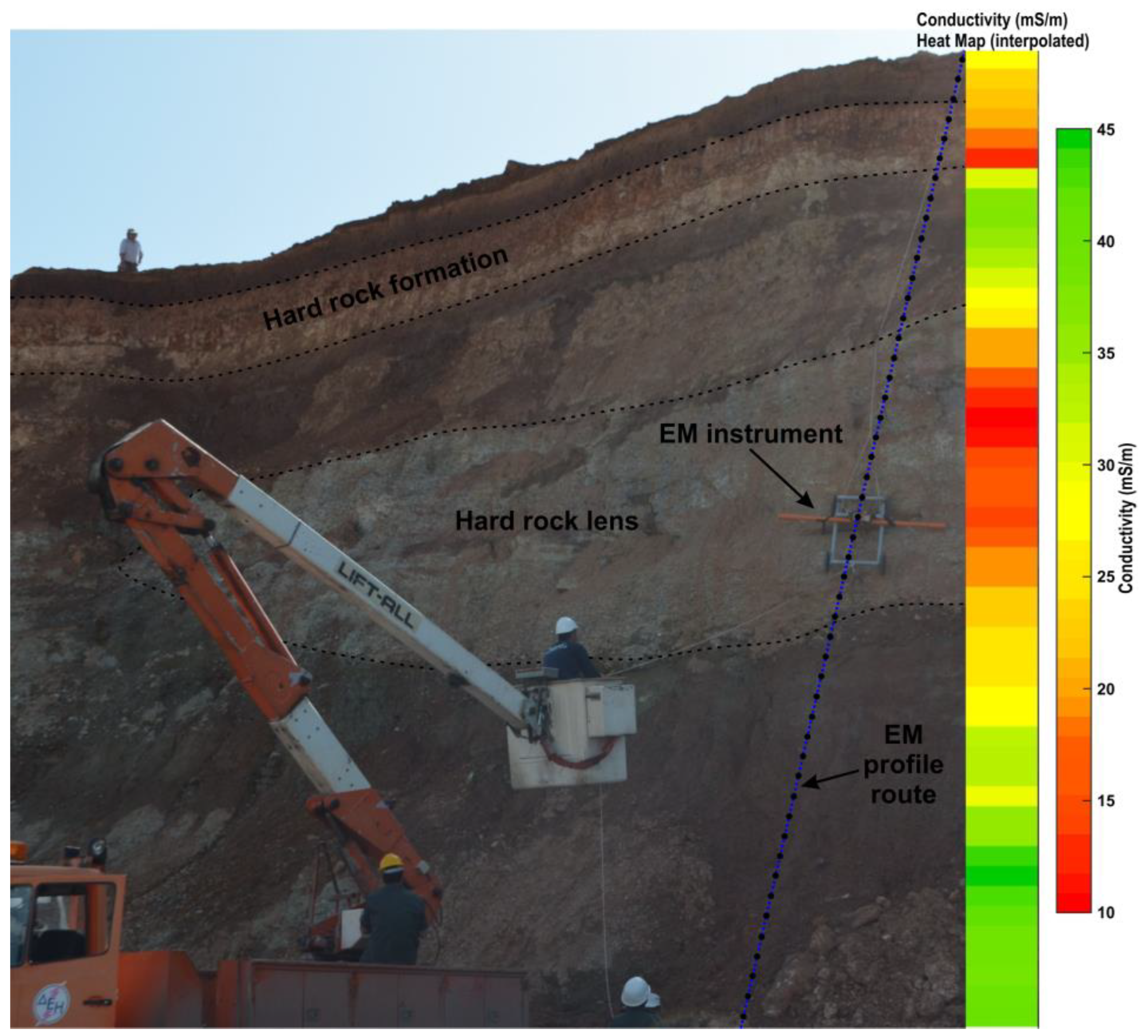More recent studies [27] have shown that the Slingram Electro-Magnetic (EM) method is feasible for unmineable inclusions detection (Figure 1). EM penetration depth and resolution are sufficient for hard rock inclusion real-time monitoring. In addition, sufficient resistivity contrast is observed between the target (hard rock) and the surrounding materials (soil) [28].

However, hard rock inclusion detection during BWE excavation is not enough. In order to retain a high level of the excavation productivity of soft materials containing hard inclusions, a decision-making system for optimum BWE collision prevention must be completed as well. Fuzzy inference systems (FIS) have been applied with success in mining [29,30]. Hence, a fuzzy inference system (FIS) is suggested to support the BWE operator in preventing collisions between the excavating buckets and the hard rock inclusions. FIS possesses the capability to handle imprecise or incomplete information and integrate it into the decision-making processes, relying on the expertise of an experienced professional [31].

The proposed automatic detection system can contribute to the optimization of mining operations by improving the resource efficiency of the produced material, the consumed materials required for the excavation (steel, electricity consumption, grease, explosives, etc.), and personnel safety. In the case of a collision with an unmineable inclusion, the excavator is not only deactivated for a short or long period, but also there is a high risk of an accident [12]. Additionally, by preventing collisions, the proposed automatic detection system can reduce the risk of damage to equipment, which is costly to repair or replace, while it can be a tool for the operator to schedule the excavation sequence effectively and for the engineer to make efficient mine planning and design, leading to the optimization of material extraction.

2. Description of the Proposed System Components

For an automatic unmineable inclusion detection and collision prevention system, a geophysical sensor, a processing tool, and a visual or sound output can be considered as the minimum requirements. Within the framework of the proposed methodology, a more sophisticated scheme is attempted. Specifically, Figure 2 shows the block diagram of the proposed system. It consists of one kinematic GPS module for accurate sensor positioning and one EM sensor (CMD2—GF Instruments) mounted on the bucket wheel boom with their corresponding control units placed in the cabin of the BWE. The EM control unit receives GPS data and exports time-stamped and coordinated resistivity values.

A frame was constructed to mount the sensor on the slewing boom with its nearest to the sensor parts made by wood beams to avoid influencing EM measurements. This frame keeps the EM sensor 5 m away from the bucket wheel and adjustable 0.5–2 m away from the mine face. Figure 3 (top left) shows the final implementation of the mounting frame with the CMD-2 and the GPS antenna attached. In addition, a CCD camera was placed on the BWE tower in order to allow the BWE operator the visual inspection of the sensor system. Furthermore, the proposed system is equipped with a fully rugged laptop placed next to the BWE operator for real-time data processing and results visualization.

As indicated in Figure 2, the EM sensor and GPS antenna transmit data to the corresponding control units. Coordinated resistivity data are transmitted at a predefined rate from the EM control unit to the laptop. A typical sampling rate of 1 sample per second corresponds to a spatial resolution of approximately 4 to 10 samples/m for a slewing speed of 15 to 6 m/min, respectively. Then, preprocessing algorithms smooth and correct the original data for extreme values. Afterward, the preprocessed data are handled either using the Simple or the Advanced Processing Mode.

Simple processing Mode uses only the last 21 resistivity values to evaluate the short-term to long-term resistivity ratio (STA/LTA) and transmits an alarm signal (high risk of collision) to the visualization unit if some predefined thresholds are exceeded. This mode is more suitable for a very short-term (on a scale of 30 s) prediction of high resistivity geophysical anomalies with a small advance in the current cut, next to BW, and is the tool for anomalies detection during the initial three cuts in each layer. As long as EM data from successive cuts have been collected, the processing is automatically switched to the Advanced Mode, which, together with the Expert System (FIS), predicts the risk of collision and the diggability for the next cuts.

The Advanced Mode is more suitable to detect resistivity anomalies related to smaller targets but with higher advance ahead of the BW. In this mode, the coordinated resistivity data from successive sensor scans are used for enhanced accuracy in unmineable inclusion detection. Apparent resistivity data from individual slewing movements are attributed to profiles and are aligned using the coordinates from GPS. Resistivity local maxima are observed in positions where hard rock inclusions exist. Their values increase as the sensor successively approaches the inclusions. Along successive profiles, the most prominent apparent resistivity peaks are detected using the Position Prominence Index (PPI) [32]. PPI is calculated from the resistivity local maxima values and their relative positions along the slewing trajectory of the successive profiles. PPI value at a specific (within a tolerance range) position continuously increases when the resistivity peak values increase in successive EM sensor scans. An updated PPI value from the previous profile, together with the apparent resistivity values from the last “n” previous profiles and the distance between successive profiles, are used as inputs in the Neural Network-based Pattern Recognition (NNPR) algorithm. This algorithm assesses the likelihood of encountering a hard rock inclusion at a particular position, “S”, along the slewing trajectory. It considers factors such as the distance between the bucket wheel and “S” and the slewing speed of the BWE boom.

The NNPR outputs, as well as the resistivity values, are used as inputs in a decision-support process based on the fuzzy inference system (FIS). The goal for the successful design of a fuzzy inference system is to capture the knowledge of a human expert relative to some specific domain and code this in a computer in such a way that the knowledge of the expert is available to a less experienced user [31,33]. The training of the FIS system is required as well and is based on synthetic data. The outputs from the FIS system to the visualization unit are the risk of collision and the diggability, ranked on a 5-level scale.

A graphical user interface (visualization unit) provides selected information to the operator of the BWE in a simple and comprehensive way (Figure 3). This unit allows the BWE operator to control the proposed system and provides basic information, such as: (a) the real-time visualization of the excavated bench face from the CCD camera, (b) visual color levels of the probability, the risk of collision (with sound warnings in the cases of high values) and the diggability, as well as (c) real-time measurements (i.e., bucket wheel position and speed, conductivity or resistivity measurements, etc.) depending on the active processing mode (simple or advanced).

The proposed methodology was extensively tested using synthetic EM data. A comprehensive description of EM data modeling is provided below. Real data acquired with a CMD2 (GF Instruments) EM instrument equipped with GPS were used to control its efficiency.

3. Electromagnetic Theory and Data Modeling

The ground conductivity instruments consist of Transmitter (T) and Receiver (R) coils. Low frequency (less than a few thousand hertz) alternating current passing through the transmitter coil creates an alternating primary magnetic field (H_p) [34]. H_p penetrates into the ground (up to a depth called skin depth) and induces conducting bodies alternating currents (eddy currents). This field, in turn, generates a secondary electromagnetic field (H_s) that travels back to the receiver. Hs has the same frequency but different phase and amplitude values compared to the primary field. These differences between the transmitted and received electromagnetic fields provide information about the geometry and electrical conductivity (σ_a in S/m) of the conductor [35]. For horizontally stratified homogeneous layers (1D media) and short coil spacings, σ_a can be calculated by the weighted (to the depth divided by the coil separation) average of the conductivities of each layer [28]. These weights (cumulative sensitivity) depend on the orientation of the coils for vertical and horizontal coil orientation.

In the case of laterally varying media, 2D effects must be considered. Thus, we propose 2D weights, which are modifications of the 1D ones. In 2D media approximation, a conductivity model is discretized in cells of constant conductivity values. The apparent conductivity is estimated by adding the contribution of each cell’s conductivity independently, weighted according to its distance from the instrument. The proposed 2D weights (2D cumulative sensitivity) were tested using both analytical 2D profiles (semi-infinite vertical sheet) as well as 1D media [36]. Namely, the 2D cumulative sensitivity matrix provides the corresponding 1D solution in the case of a 1D medium.

Figure 4a illustrates the cumulative sensitivity weighting factor for the CMD2 instrument utilized in this study, considering a coil spacing of 1.89 m, low depth range mode (horizontal coil axes), and a maximum depth of EM signal penetration equal to 7 m. Additionally, Figure 4b displays the synthetic apparent resistivity (ρ_a = 1/σ_a) profiles corresponding to both 1D and 2D approaches. These profiles depict a model comprising a conductive half-space, which includes two non-conductive bodies. Normally distributed pseudorandom numbers with zero mean and standard deviation of 20% of the half space conductivity were created using the “randn” MATLAB function and were added to model conductivity values.

Different resistivity profiles are calculated for each model by decreasing the depth of the boulders with a step equal to the BW cut advance. This resamples the BW approach towards the boulders as the excavator advances forward with a fixed step for each cut.

Synthetic EM Data Adjustment on Bucket Wheel Terrace Cutting

At the beginning of the project, due to the lack of real data, we simulated the bucket wheel movement during a standard block excavation by a BWE applying terrace cutting. Figure 5 displays the synthetic X, Y, and Z (elevation) coordinates (in UTM) obtained from both the BWE and CMD2 trajectories. Random noise with a standard deviation of 0.1 m in X-Y and 0.3 m in Z direction was added to trajectory positioning. In order to gather the measured (along the BW trajectories) apparent resistivity data over an orthogonal synthetic resistivity model (i.e., see Figure 4b), we first calculated an apparent resistivity map (Figure 6b) by gradually burying the targets with very small depth steps. This is the same as gradually placing the EM sensor away from the targets. On this map, we selected the nearest to BW slewing trajectories resistivity values (colored paths in Figure 6b) in order to form the measured resistivity profiles (Figure 6a). Following that, after considering the simulated excavation process, we developed an algorithm to segment and arrange the synthetic or real data into blocks, layers, and cuts. This enables us to generate successive resistivity profiles, which were used as the input data for the Advanced Mode algorithm.

4. Data Processing

The positioned EM data are transmitted in continuous mode at predefined sampling intervals from the EM control unit to the serial port of the rugged laptop in the BWE operator cabin. The original data are subjected to preprocessing, which consists of (a) coordinate data transformation (latitude, longitude, altitude to UTM X, Y, Z), (b) outlier values removal, and (c) data smoothing. Two distinct algorithms have been created: one, relatively simpe, which named “Simple Mode”, which relies on statistical process control, and another one, more advanced, referred to as “Advanced Mode”. The Advanced Mode algorithm utilizes Position Prominence Index (PPI) and Neural Network-based Pattern Recognition (NNPR) to enhance its capabilities.

4.1. Simple Mode Algorithm

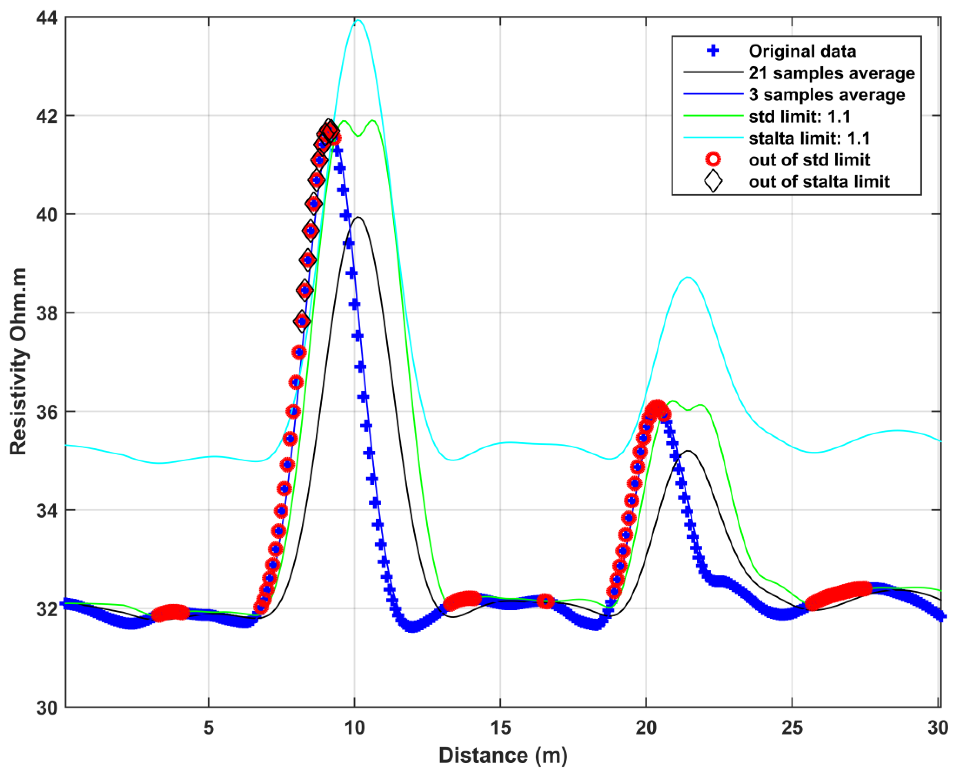
The algorithm in Simple Mode for Hard Rock Detection (SMHRD) relies on statistical process control and utilizes data obtained during the ongoing cut performed by the BWE. SMHRD algorithm utilizes a moving average operator, applied both on the latest 21 (Long Term Average—LTA) and 3 (Short Term Average—STA) preprocessed resistivity values. Both STA and LTA values are attributed to the last measured point (eccentric mean value). An alarm indicator is issued if both the STA value exceeds a predefined limit of long-term data window standard deviation (STD) and the STA/LTA ratio exceeds its predefined limit, respectively. The optimal data windows for STA (3) and LTA (21), as well as the predefined limits for STD (1.1) and the STA/LTA (1.1) ratio, were determined through the performance evaluation of the SMHRD algorithm using 100 different randomly generated 1-boulder models and 100 2-boulder models [37]. Figure 7 shows an example of SMHRD algorithm application on the synthetic resistivity values deduced from the model presented in Figure 4b. Both the limits for the standard deviation and the ratio of the STA/LTA multiplication factor are set to 1.1. In this case, the algorithm issued an alarm from 8.2 to 9.2 m of profile, where the STA value (blue curve in Figure 7) exceeds both 1.1 times the current long-term data window STD value (green curve in Figure 7) and 1.1 times the STA/LTA ratio (cyan curve in Figure 7).

The SMHRD algorithm generates a relatively high rate of false alarms when dealing with two-boulder models, mostly due to the detection of deeper and occasionally larger structures with higher resistivity, as demonstrated in Figure 7, as well as suffers from early warning alerts, by issuing alerts several slices ahead [37].

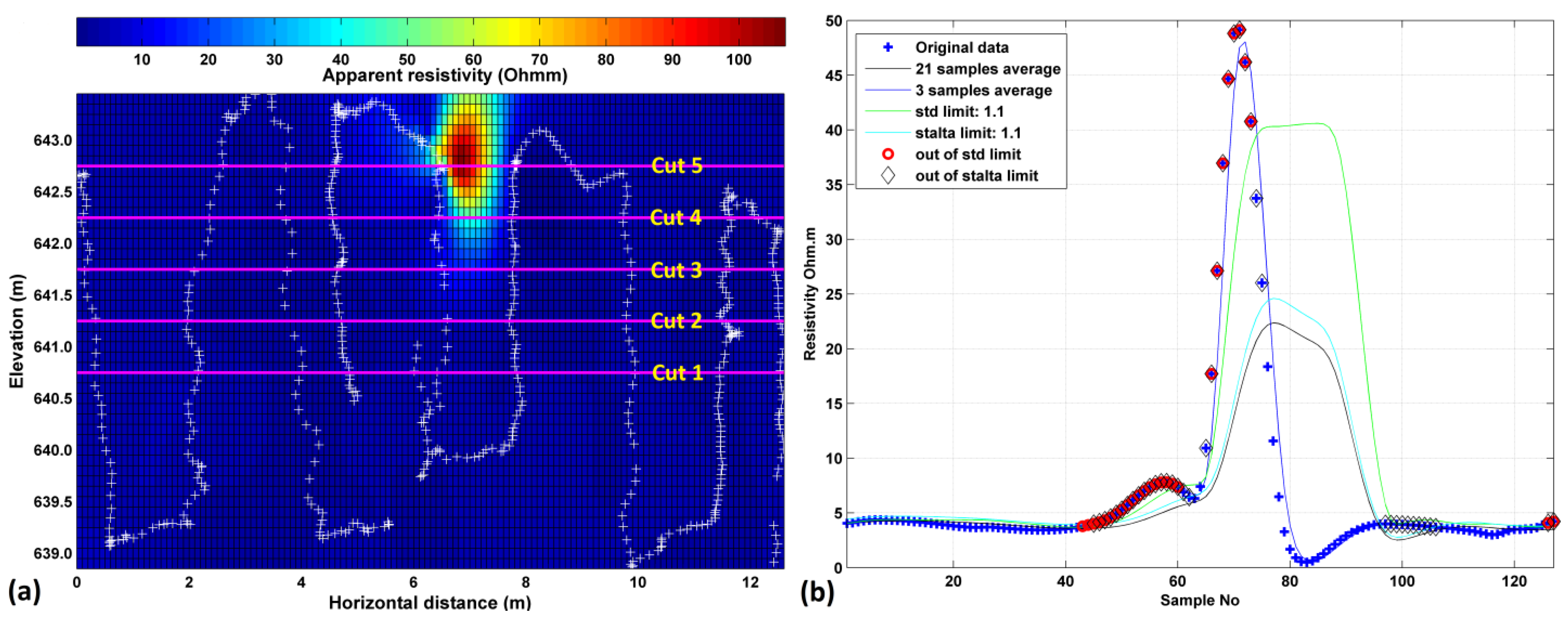
Figure 8a shows a map illustrating the experimental apparent resistivity values obtained in June 2017 from the South Field open pit mine in Ptolemaida, Greece. The data was collected by moving the CMD2 instrument mounted on a bucket truck along a slope (Figure 1). Within the clays, there were hard rock inclusions in the form of layers or thin lenses. The map in Figure 8a was generated through interpolation of the apparent resistivity values collected from the CMD2 instrument along the route marked with white crosses. The area with higher resistivity values (>70 Ωm) corresponds to the region where we visually observed hard rock inclusions.

To further analyze the data, separate datasets were extracted from five resistivity profiles spaced 0.5 m apart, representing successive cuts made by the bucket wheel excavator (cut 1–5). Figure 8b presents an example of the SMHRD application specifically for the 4th cut based on the aforementioned experimental data. This cut is considered to be the one immediately preceding the bucket wheel’s encounter with the boulder (which occurs at the 7 m along the fifth cut). In this figure, warning alerts are indicated in regions where the STA value exceeds both the standard deviation and STA/LTA predefined limits, coinciding with a sharp increase in resistivity values.

4.2. Advanced Mode Operation Algorithms

Advanced Mode operation requires the EM data to be organized in apparent resistivity profiles (horizontal distance versus apparent resistivity). As the CMD2 instrument is positioned adjacent to the bucket wheel at a specific distance, its trajectory exhibits a cyclical pattern that aligns with the slewing motion of the bucket wheel. Data collected along a slewing cut are attributed to a resistivity profile. Successive profiles are the input data for Advanced Mode operation. For that reason, accurate positioning of the EM instrument is essential to break down the EM data into resistivity profiles.

4.2.1. Position Prominence Index (PPI)

Apparent resistivity values are anticipated to be gradually increased in the vicinity of hard rock inclusions as the EM sensor approaches them. Thus, gradually increasing local resistivity maxima in successive resistivity profiles should be a very good indicator for detecting and positioning the targets. Based on that assumption, we apply an algorithm for the recognition of the most prominent resistivity peaks in successive apparent resistivity profiles.

The local maxima of a resistivity profile are defined as the positions where their values are higher than the ones of the neighboring positions. The global maximum (the local maximum with the highest resistivity value) is ranked as the first peak. Subsequently, the following peaks are recursively ranked based on their proximity to the previous ones. For each local maximum, the algorithm traces the path back to the previous peak within the data. The prominence of a local maximum is determined by calculating the difference between the maximum and minimum resistivity values along this path. The peak with the highest prominence is designated as the next prominent peak. It should be noted that as the required number of peaks increases, this algorithm will yield maxima with lower prominence values.

The user defines the Number of Local Maxima (NLM), and the algorithm ranks the NLM local maxima of a certain apparent resistivity profile in Prominence Ranks (PR). The Position Prominence Index (PPI) is calculated using the formula.:

$$\mathit{PPT}=\frac{\mathit{NLM}}{\mathit{PR}}$$

(1)

Figure 9a shows the application of the PPI algorithm on the synthetic data deduced from the synthetic model shown in Figure 4b. Ten NLM points (if they existed in the data) were used (PPI-10). The higher resistivity targets (boulders) were initially placed 4 m deeper than the depth shown in Figure 4b and successively moved toward the free surface with steps equal to 0.5 m (simulating a fixed BW advance). The corresponding apparent resistivity values of profiles one to eight were introduced as input in the PPI algorithm. The apparent resistivity values shown in Figure 9a correspond to the last two profiles (pass seven and eight), while PPI corresponds to the last profile. However, its values are the outcome of the successive update of PPI values from profiles one to eight. Further details concerning the way PPI values are upgraded during successive cuts can be found in [37]. The PPI profile in Figure 9a indicates two dominant peaks at approximately 7 and 20 m with values of 18 and 106, respectively. Notice that the SMHRD algorithm, applied on the last profile data (number eight) of the same model, failed to detect the shallower (but smaller) target located approximately at the position of 20 m (see Figure 7). On the other hand, the PPI algorithm not only managed to detect both of the targets but highlights (with higher PPI values) the shallower (and smaller) target as the primary target for issuing a collision alarm. Figure 9b displays the outcome of the application of the PPI algorithm on the real data shown in Figure 8. The corresponding apparent resistivity values of profiles one to five were introduced as input in the PPI algorithm. The apparent resistivity values shown in Figure 9b correspond to the profiles from cut two and three (pass four and five, respectively, in Figure 9b), while PPI corresponds to third profile. There is one dominant at approximately 7 m distance and several others with smaller PPI peaks. The smaller difference in PPI values between the target and the other PPI peaks is attributed to the fact that random and/or coherent noise level is higher in real apparent resistivity data compared to the synthetic ones.

PPI proved an excellent position boulder detector technique and is used as input in the Neural Network-based Pattern Recognition (NNPR) algorithm to increase the success rate of hard rock inclusion detection. Nevertheless, this approach has two primary limitations: (a) it is susceptible to errors in measurement positioning, and (b) establishing a standardized threshold for the Position Prominence Index (PPI) is challenging due to its dependence on the number of data points in the profiles.

4.2.2. Automatic Evaluation of EM Profiles Based on Artificial Neural Networks for Pattern Recognition

The developed neural network model, known as Neural Network for Resistivity Pattern Recognition (NNRPR), is a feedforward neural network with a hidden layer containing 10 neurons. The prediction is based on analyzing local variations in resistivity profiles generated by the EM sensor (CMD2) mounted on the bucket wheel during the excavation process and the distance between the analyzed local resistivity profiles at the position x_o, y_o, z_o. NNRPR utilizes a moving window that includes k resistivity and PPI values, which correspond to the same positions along n successive cuts, to estimate the likelihood of encountering a hard rock formation in the subsequent cut (n + 1) at a specific position x_o, y_o, z_o, as depicted in Figure 10. During terrace cutting (Figure 10a), as the bucket wheel approaches the hard rock formations, the resistivity values exhibit an increase due to the presence of the hard rock formation. These patterns in the resistivity profiles serve as indicators of the existence of a hard rock formation, as depicted in Figure 10b. After training, the NNRPR neural network model is capable of recognizing these patterns (increasing resistivity and PPI values in successive profiles) and associating them with the position of the hard rock formation.

Throughout the training and testing stages of NNRPR, using a large set of synthetic data (178,200 cases) from models with one or two hard rock inclusions of varying sizes, shapes, and positions, multiple combinations of n and k values were assessed, and the optimal values determined to be n = 3 and k = 5. The synthetic data was randomly split into three distinct datasets: the training set, which comprised 70% of the total data; the validation set, consisting of 15%; and the testing set, consisting, as well, of 15%. The validation dataset was used to prevent overfitting through the utilization of the early stopping technique, while the testing dataset was used to assess the network’s ability to generalize.

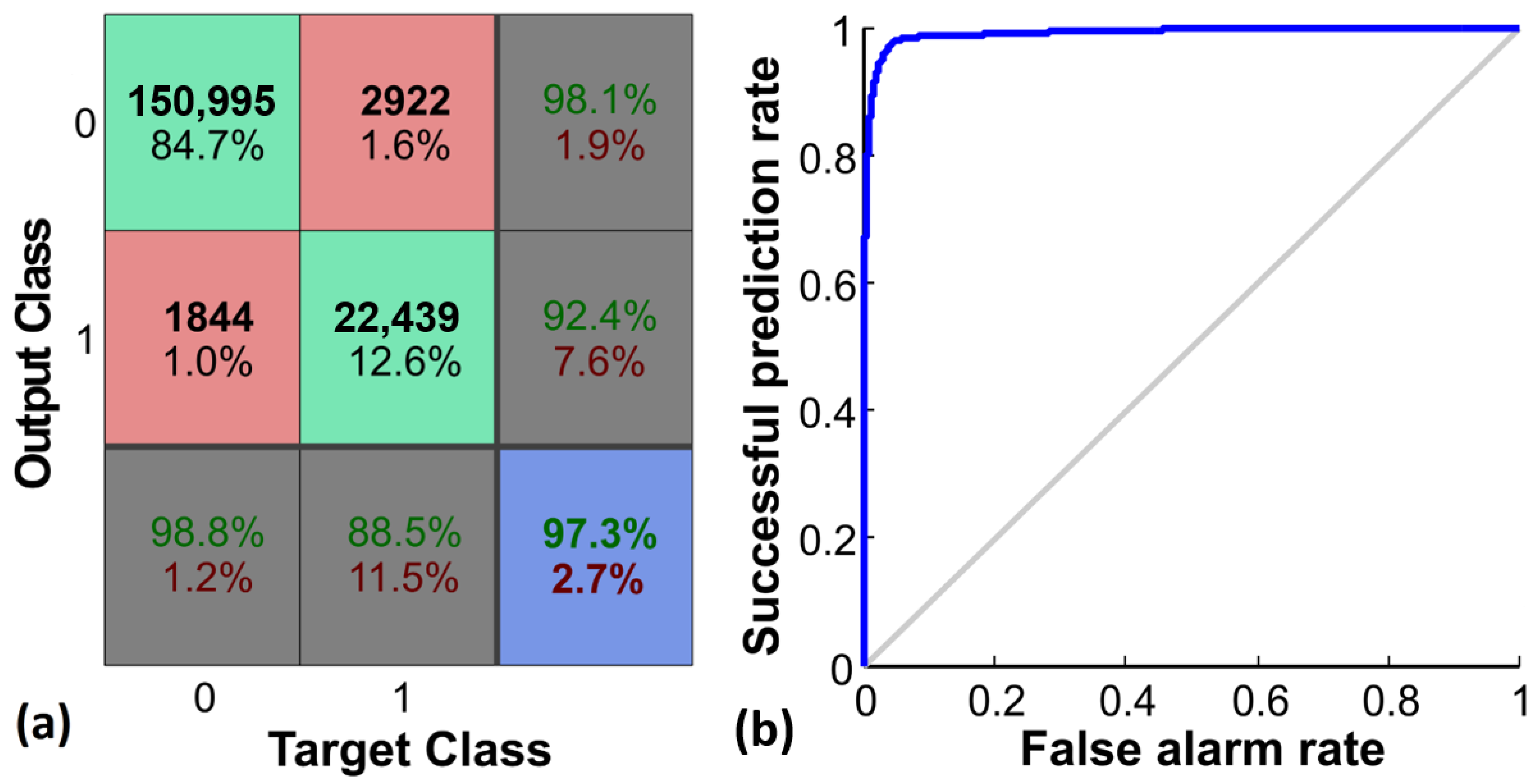
NNRPR was developed, trained, and tested using the MATLAB^TM. The resulting confusion matrix from NNRPR training is displayed in Figure 11a. The matrix presents both the absolute numbers and the percentages of accurate predictions (highlighted in green) and false predictions (highlighted in red). In this matrix, class 1 represents the presence of a hard rock inclusion, while class 0 represents its absence. There are four different conditions: (0-0), (1-1), (0-1), (1-0). The first number in the parentheses corresponds to the fact, while the second corresponds to the NNRPR result. The top-left four colored panels and the bottom right blue one correspond to the true (green) and false (red) predictions for the total input data. Similarly, the predictions for the validation data are given in the right grey column, while the predictions for the testing data are in the bottom grey row.

The percentage of successful hard rock inclusion existence predictions in testing data is 88.5% (11.5% were missed), while the percentage of false alarms is only 1.2%. Taking into consideration the relatively high percentage (24,283 cases out of 178,200) of hard rock inclusion existence in the synthetic data, these percentages are considered acceptable. In Figure 11b, the Receiver-Operator Curve (ROC) is presented, demonstrating the relationship between the false alarm rate and the rate of successful predictions. It is evident from the ROC that achieving a higher rate of successful predictions (e.g., 0.98) may lead to a significant increase in the false alarm rate (0.1). In other words, since the occurrences of boulders in the open pit mines are quite rare, a very low false alarm and a high true alarm rate (i.e., 1.2% and 88.5%) is preferable, rather than a very high true alarm and a relatively low false alarm rate (i.e., 98.0% and 10.0%).

Using the trained NNRPR, predictions were made regarding the presence of hard rock formations in real data, as illustrated in Figure 8. The apparent resistivity values from the five successive cuts (cuts 1–5 in Figure 8) were utilized as input to NNRPR for estimating the probability of encountering a hard rock formation. The calculated probabilities along the resistivity profiles for each cut are displayed in Figure 12. NNRPR predicted a probability of 0.92 for the occurrence of a hard rock formation at 7 m of the 5th cut. Conversely, in previous cuts (1–4), the predicted probabilities were considerably low, almost approaching zero.

5. Fuzzy Inference System

In contrast to the conventional Boolean set that only permits values of 0 or 1, a fuzzy inference system (FIS) employs continuous boundary values that enable partial membership. The extent of membership in a set is represented by a number ranging from 0 to 1, where 0 signifies complete exclusion from the set, 1 denotes full inclusion in the set, while values in between indicate partial participation within the set.

For the development of the FIS, the Fuzzy Logic Toolbox of the Mathworks was implemented [38]. The steps for the development of the FIS were: (1) Definition of the input/output and fuzzification variables, (2) creation of the inference rules (application of the fuzzy operator (AND, OR) in the antecedent and implication from the antecedent to the consequent), (3) Aggregation of the consequents across the rules and (4) Defuzzification.

Based on the assessment of mining operations and expert opinions, the developed Fuzzy Inference System (FIS) incorporates four inputs:

(1)

The probability of encountering a hard rock formation at a specific position S, represented by fuzzy variables such as low, medium, and high.

(2)

The distance between the bucket wheel and position S, categorized into fuzzy variables such as small, medium, and large.

(3)

The slewing speed of the bucket wheel, characterized by fuzzy variables, including low and high.

(4)

The apparent resistivity values of the excavated material, classified as fuzzy variables such as low, medium, and high.

FIS comprises two outputs:

(1)

The risk level of the bucket wheel colliding with a hard rock formation, expressed through fuzzy variables such as low, average, and high.

(2)

The diggability assessment of the excavated formation, categorized into fuzzy variables such as easy, average, and difficult.

Overall, the FIS utilizes these inputs and outputs to analyze and make informed decisions based on the given mining conditions and expert insights. The structure of the FIS, consisting of four inputs, two outputs, and 12 rules, is shown in Figure 13. The rules of the FIS were derived from the collected knowledge and experience of mining engineers and BWE operators. These rules were optimized during the training of the FIS. 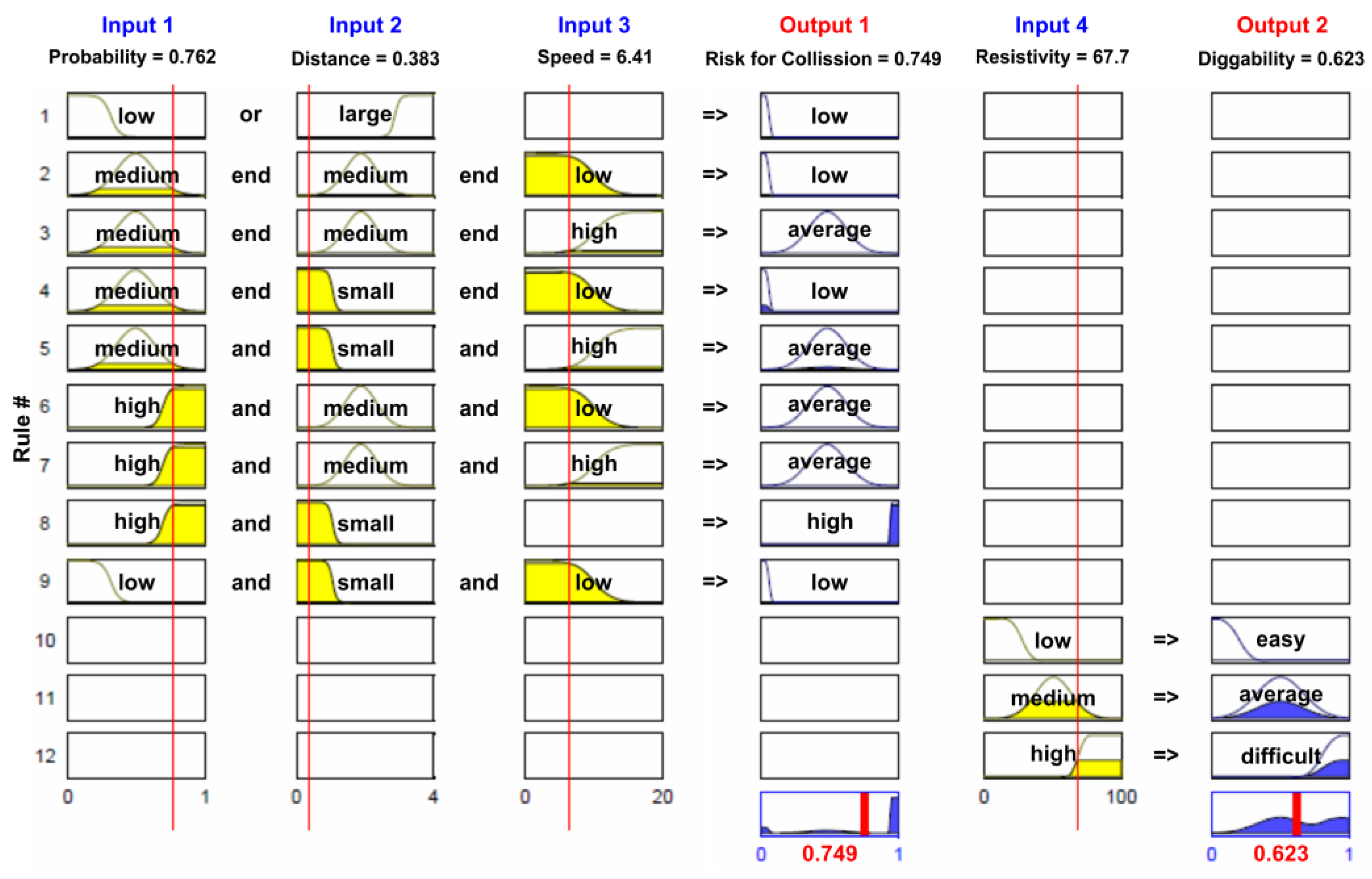Figure 14 provides a schematic depiction of the complete set of rules for the developed FIS. Except for rule 1 (with operator OR) and rules 10–12, which are solely influenced by the resistivity values, the fuzzy operator AND was applied to the other fuzzy antecedents. In the presented example (Figure 14), the probability is high (0.762), the distance is small (0.383 m), and the speed is low (6.41 m/min), resulting in an average to high risk of collision (0.749), while the resistivity is medium to high (67.7 Ωm) resulting in average diggability (0.623).

The Risk of Collision is maximized when the Probability of hard rock occurrence is high, and the Distance between the BWE and the hard rock is low (as seen in rule #8 in Figure 14). Conversely, the estimation of diggability is solely based on the measured apparent resistivity values (as observed in rules #10, 11, and 12 in Figure 14). The implementation of FIS to the proposed real-time unmineable inclusions detection system also involved the development of a graphical user interface (visualization unit in Figure 3) that presents all necessary information for the operator of the BWE.

6. Discussion

The proposed methodology aims at the automatic bucket wheel excavator collision prevention on unmineable inclusions, and thus, it cannot be directly compared to the most relative ones, which are aimed at the delineation of the stratum layer boundaries [25,26]. However, the advantages of this work can be summarized as the efficiency of data processing and interpretation. The reduced collected EM (compared to the corresponding GPR) data and their relative simplicity (one resistivity value versus GPR amplitudes over the recording time) result in the reduction of the processing time and simplify the process of automated interpretation, respectively. However, further work is required for improving the rigidity of the detection system in order to eliminate the heavy torque forces applied on long EM sensor supporting frames during the excavation. In addition, a lack of real data positioning accuracy was detected due to GPS antenna proximity to bench face. An alternative position of the GPS antenna could be on the top of the operation tower, provided that correction of the EM sensors’ positions (based on their relative position to the GPS antenna) are applied too.

In order to evaluate the impact of the proposed methodology on the improvement of the open pit mine operations sustainability, we have to take into consideration different observed parameters. Lazarević et al. [39] examined the Tamnava—West Field Open Cast Mine in Lazarevac (Serbia) system failures in the period from 2003 to 2011 and demonstrated that the BWE material digging subsystem has the most breakdowns after the material transporting subsystem. The same study showed that failure rate, λ(t), is a constant function of time, and the reliability of an SchRs 900.25/6 excavator can be approximated by the exponential distribution. For the year 2011, the mean failure rate function for the material digging subsystem was evaluated as λ(t) = 0.0024 t, with time (t) units in hours. According to Huss [12], 13% of machine breakdowns in Polish open pit mines are a result of extreme geological conditions. As much of this happens because of the maladjustment of mining technology to the above-mentioned circumstances, leading, totally, to above 25% of all breakdowns. During December 2018, in the South Field open-pit mine, Ptolemaida, Greece, the BW excavator of the upper terrace (where the hard rock formations exist) recorded 237.1 hours of breakdown alone, while the corresponding one from the lower terrace recorded only 52.6 h.

Electricity consumption of the BW is strongly related to the bucket load. Between 60 and 90% of the electricity is consumed by BW excavators to cut and remove the material [40]. As a result, it is very important to reduce this component of power consumption, which is attributed to hard rock inclusions. However, this can be traditionally achieved by blasting the hard rock formation prior to the excavation. Kumaraswamy and Mozumbar [41] note that by adding a blasting step to the excavation of hard overburden formations, the productivity of the BWE had a 15.4% increment with a simultaneous 22% reduction of BW load in the Neyveli mine (India).

Sustainable mining is closely connected with the main objectives of mining operations, which are related, among others, to rational exploitation, the optimization of productivity and cost savings, the elimination of deviations from quality specifications, and zero accidents. The proposed methodology is an automated process, which could significantly contribute to the maintenance of the production planning, especially of the upper terraces progress, where the hard rock formations are encountered. This eventually results not only in avoiding coal production delays due to the corresponding overburden exploitation delays but also reduces the operations of blasting and removing the hard rock formations, which require high-cost diesel equipment.

7. Conclusions

Summarizing this work, we have developed a promising methodology for automatic bucket wheel excavator collision prevention on unmineable inclusions, using positioned electromagnetic (EM) inspection and a fuzzy inference system. The proposed operation flowchart consists of the following tasks: (1) continuous EM and GPS data collection, (2) data preprocessing, (3) unmineable inclusion detection, and (4) decision support system and visualization. In this study, a novel system was created as a tool for the operator and the engineer to mitigate the negative effects of hard formation excavation as an emergency tool to immediately alarm the operator, as well as a tool for short to mid-term optimization of mine planning.

Two distinct evaluation approaches were investigated for the automatic detection of hard rock inclusions. The first approach referred to as Simple Mode, relies on statistical process control, while the second approach, known as Advanced Mode, is more sophisticated and utilizes both Position Prominence Index (PPI) and Neural Network-based Pattern Recognition (NNPR). Extensive testing was conducted on both methods using synthetic data to assess their effectiveness. Additionally, real data was gathered from field tests employing a bucket truck and an EM sensor mounted on the boom of the bucket wheel during excavation field tests. Comparing the two approaches, the Advanced Mode exhibited enhanced accuracy in automatically detecting unmineable inclusions when compared to the Simple Mode. However, it should be noted that the Advanced Mode is sensitive to positioning accuracy and necessitates appropriately sorted EM data from a minimum of three successive cuts of the bucket wheel excavator. Thus, it is suitable for hard rock detection in the next cuts and blocks, which is valuable for short to mid-term mine planning. On the other hand, Simple Mode is independent of instrument positioning and more robust. It can be used easily by the operator of the BWE in real time for the early detection of the hard formations encountered in the slice under excavation.

The use of fuzzy logic allowed capturing and incorporating the existing experiential knowledge about excavated material properties and the mining with BWE in a very efficient way in the developed fuzzy expert system used to estimate the risk of collision of the bucket wheel with hard rock formations. The use of fuzzy logic results in the gradual detection of collision, and this was very convenient for BWE operators. Furthermore, the developed fuzzy expert system can be simply adjusted through membership functions to include new factual knowledge, while the fuzzy set of rules can be easily extended to incorporate additional experiential knowledge. This will allow the application of the developed system in different mining environments.

As presented in the discussion part, the proposed methodology can contribute to the optimization of mine operations by improving resource efficiency, safety, cost savings, and environmental sustainability.