Article

Assessing Soil Erosion Susceptibility for Past and Future Scenarios in Semiarid Mediterranean Agroecosystems

by
Gianluigi Busico
1,*,
Eleonora Grilli
1,
Silvia C. P. Carvalho
2,
Micòl Mastrocicco
1 and
Simona Castaldi
1
1
Department of Environmental, Biological and Pharmaceutical Sciences and Technologies, University of Campania “Luigi Vanvitelli”, 81100 Caserta, Italy
2
Faculty of Sciences, CCIAM (CC Impacts Adaptation & Modelling), cE3c, University of Lisbon, 1649-004 Lisbon, Portugal
*
Author to whom correspondence should be addressed.
Sustainability 2023, 15(17), 12992; https://doi.org/10.3390/su151712992
Submission received: 24 June 2023 / Revised: 31 July 2023 / Accepted: 25 August 2023 / Published: 29 August 2023

Abstract

:
The evaluation of soil erosion rate, particularly in agricultural lands, is a crucial tool for long-term land management planning. This research utilized the soil and water assessment tool (SWAT) model to simulate soil erosion in a semiarid watershed located in South Portugal. To understand the evolution of the erosive phenomenon over time, soil erosion susceptibility maps for both historical and future periods were created. The historical period exhibited the highest average soil erosion for each land use, followed by the representative concentration pathways (RCPs) 8.5 and 4.5 scenarios. The differences in soil loss between these two RCPs were influenced by the slightly increasing trend of extreme events, particularly notable in RCP 8.5, leading to a higher maximum value of soil erosion. The research highlighted a tendency towards erosion in the agroforestry system known as “montado”, specifically on Leptosols throughout the entire basin. The study confirmed that Leptosols are most susceptible to sediment loss due to their inherent characteristics. Additionally, both “montado” and farmed systems were found to negatively impact soil erosion rates if appropriate antierosion measures are not adopted. This underscores the importance of identifying all factors responsible for land degradation in Mediterranean watersheds. In conclusion, the study highlighted the significance of assessing soil erosion rates in agricultural areas for effective land management planning in the long run. The utilization of the SWAT model and the creation of susceptibility maps provide valuable insights into the erosive phenomenon’s dynamics, urging the implementation of antierosion strategies to protect the soil and combat land degradation in the region.

1. Introduction

Soil erosion (SE) is a major environmental concern in arid and semiarid regions, especially in agricultural areas, which now have the highest average rate of soil loss worldwide [1]. SE is the main driver of land degradation and desertification, with the consequent loss of ecosystem services [2,3,4]. The rate of SE is generally controlled by many factors and processes, such as wind, water input and balance, vegetation cover, geomorphology, soil type, and anthropogenic activities [5,6]. On a global scale, rainfall frequency and duration are widely recognized as the most important drivers of observed and modelled SE rates [7,8]. Over the past century, the rate of SE has risen sharply, resulting in a global average soil loss rate of around 10.2 t/ha/year, projected to rise by 14% by the end of the 21st century [9], with climate change (CC) playing a major role in determining the extent of SE [10]. In this context, the Mediterranean region has been recognized as highly susceptible to SE, making it a climate change ‘hot-spot’. The region faces significant challenges due to the projected rise in temperature and disruptions in rainfall patterns [11,12,13]. These climate change impacts include more frequent extreme events, intensified storms, prolonged periods of drought, and an elevated risk of fire occurrences [14,15]. In addition, the Mediterranean region is also characterized by centuries of anthropogenic disturbance, mainly in relation to agricultural and silvopastoral activities, which could be a contributory factor to a significant increase in SE rates [16]. SE is a serious environmental and economic problem in several European countries. It has been reported that 12 million hectares of agricultural land suffers from severe erosion, resulting in yield and economic losses.
Here, adverse extreme events, such as long periods of drought followed by heavy rainfall, can exacerbate erosion to the point of irreversibility [17].
SE is also exacerbated by human activities, such as deforestation, overgrazing, poor agricultural practices, and construction [18], becoming unsustainable when the rate of soil loss exceeds the rate of soil formation.
A reliable quantitative assessment of SE is a prerequisite for land management planning and policies for the halting and reversal of land degradation. Among the available tools, the empirical universal soil loss equation (USLE) [19] and its revised version (RUSLE) [20] have been widely applied to determine the mean annual SE rates at regional and local scales [21,22,23]. Panagos et al. [24] estimated the whole set of USLE parameters for Europe, significantly improving the potential applicability of this model. Anyway, despite their wide applicability, both methodologies still limit our ability to simulate soil deposition and to determine the location of sediment sources [25]. To address the limitations of previous approaches, several river basin scale models have been developed to simulate soil erosion mechanisms and dynamics. These models include the water erosion prediction model (WEPP) [26], the Limburg soil erosion model (LISEM) [27], the European soil erosion model (EUROSEM) [28], and the soil and water assessment tool (SWAT) [29,30], which was introduced by the United States Department of Agriculture. Among these models, SWAT has gained widespread popularity due to its effectiveness in assessing hydrological responses, including water, sediment, and nutrient loss, in watersheds with diverse land covers, soil types, and management practices [31,32,33,34,35]. In recent times, SWAT’s applicability has significantly improved with the availability of an increasing number of global and regional datasets [36]. These datasets enable researchers to better calibrate and validate the model, enhancing its accuracy and allowing for a more comprehensive analysis of soil erosion dynamics in various landscapes and environmental conditions. This study aims to assess if and how CC affects SE rates in the Guadiana sub catchment, a dry area in Portugal (Alentejo), under no change in land use (business as usual, BAU) and considering two CC projection scenarios corresponding to different greenhouse gas (GHG) concentrations (RCP4.5 and RCP8.5). To achieve this objective, the operational steps of the study are (i) to produce maps of SE susceptibility for the whole catchment area, (ii) to assess its evolution over time (1980–2000, 2020–2040), and (iii) to identify the more vulnerable areas and their current land use to support local farmers in defining the most appropriate land management strategies to reduce current SE rates.

2. Materials and Methods
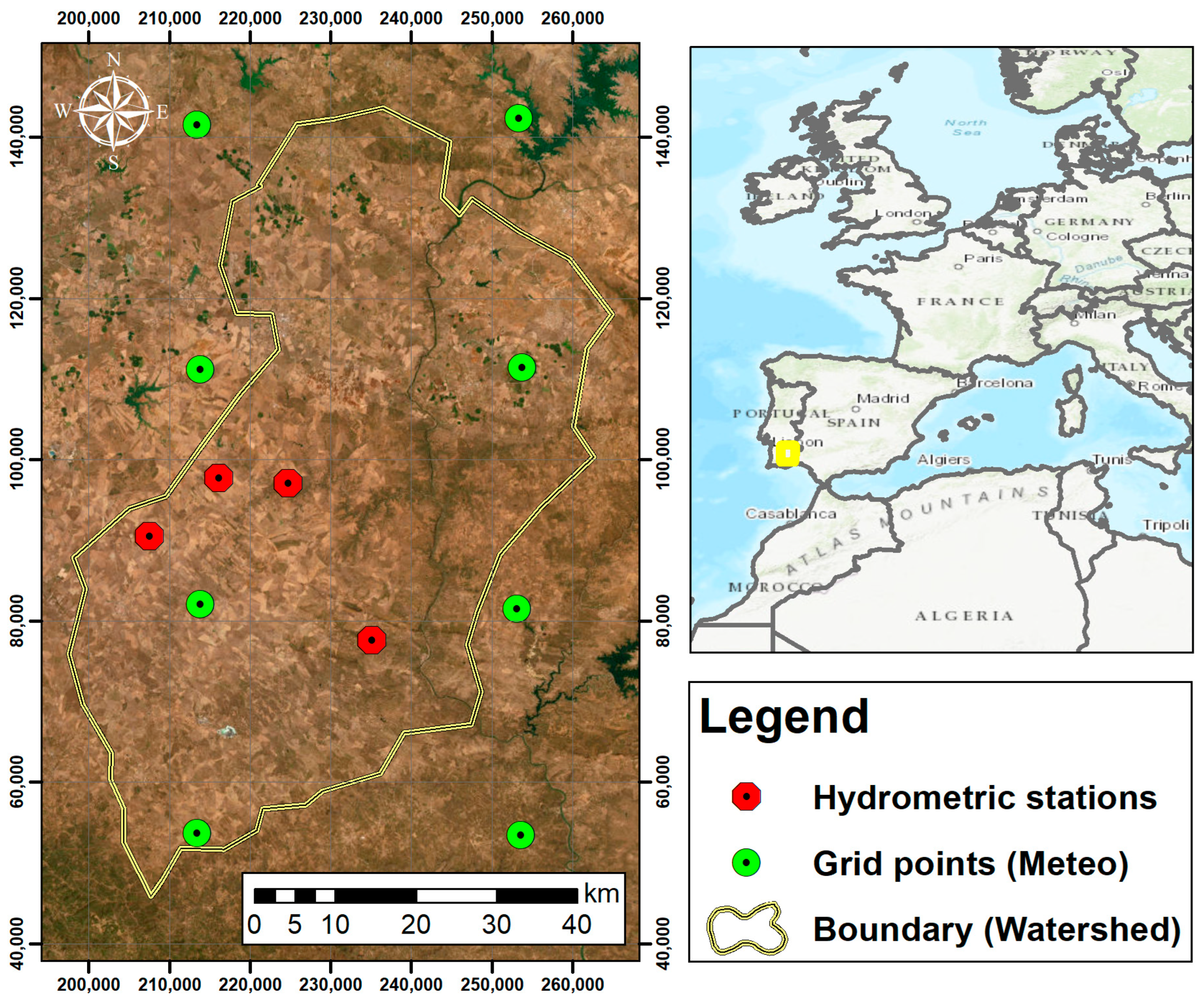
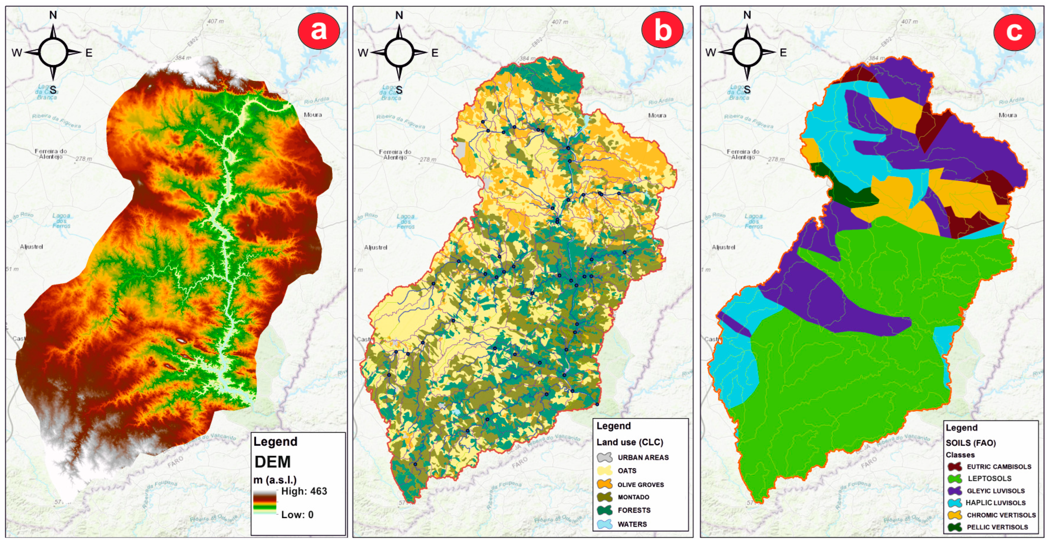
2.1. Study Area

The study area is in the Alentejo region (Figure 1), southeastern Portugal. Alentejo represents the largest region of Portugal, with a total area of about 31,500 km2 hosting 5% of the entire Portugal population. Morphologically, it is an area with relatively low reliefs, where the elevation varies from 0 to 460 m above sea level (a.s.l.) (Figure 2a). From a geological point of view, the basin mainly consists of metamorphic schists, greywackes, and conglomerates, distinguished by skeletal low productive soils [37]. The whole region has a typical Mediterranean—Continental climate, characterized by very hot and dry summers [38], with the highest amount of rain in winter and drought periods (April–September) occurring during the year (Figure S1). The lowland areas experience a mean annual precipitation ranging from 400 to 600 mm, whereas in the mountainous regions, it can reach up to 900 mm. Typically, the majority of the annual rainfall occurs within a short period of 50–75 days, mainly during the winter season [39]. The average temperature ranges from 15.0 to 17.5 °C. Additionally, the potential evapotranspiration (PET) is generally higher than 1000 mm per year, leading to a significant water–soil deficit. Three main soil groups characterize the watershed: Leptosols are the most frequent, followed by Luvisols and Vertisols [40] (Figure 2c). The prevailing land cover (Figure 2b) is represented by annual rainfed crops (wheat and oats), followed by olive groves and cork oak (Quercus suber L.) woodlands alone or in combination with Quercus ilex L. and in some cases with Mediterranean shrubs. The “montado” ecosystems, representing the traditional agroforestry system of the Iberian Peninsula with a savanna-like physiognomy, is characterized by grazing animals and by an open tree canopy woodland, which can vary between 20 and 80 trees per hectare (mainly Quercus suber, Quercus ilex subsp. rotundifolia L.) coexisting with grasses and scattered shrubs [41]. The entire region is currently at high risk of desertification due to the presence of Leptosols (Figure 2c), shallow and extremely gravelly soils that are naturally prone to erosion because of intensive agricultural management and overgrazing in recent decades [42,43]. The geomorphological, soil, and land cover characteristics of the four farms are presented in Table S1.

2.2. Data Collection

For the realization of a complete SWAT model, several datasets are required as input data. The digital elevation model (DEM), needed for the delineation of the main watershed, river network, and sub-basin generation, was provided by the Shuttle Radar Topography Mission (SRTM), with a cell resolution of 30 × 30 m. The land cover was obtained from the Corine Land Cover (CLC) database [44], while the soil classification was extracted from Direção-Geral de Agricultura e Desenvolvimento Rural (DGADR) [45] with a scale of 1:25,000 (12.5 × 12.5 m). The information on soil characteristics, such as saturated hydraulic conductivity (Ks), available water content (AWC), and bulk density (BD), was defined with the Harmonized World Soil Database [40], a vectorial geodatabase obtained from a 30” resolution map and further refined using 3000 soil columns from the World Soil Information Service [46,47,48] and literature data [3], while other missing soil’s parameters were obtained from SWAT’s default dataset (Table S2). Data on streamflow and sediment load for the period 1985–1989, used to calibrate and validate the model, were obtained from four hydrometric stations located inside the basin named Albernoa, Monte da Ponte, Oeiras, and Entradas (Figure 1) [49].

2.3. Climate Dataset

For running the model, time series of climate data, which included daily precipitation and maximum and minimum temperatures, were utilized. These climate data were obtained from the “Iberia01” dataset [50,51], which offers a dense network of weather stations across the Iberian Peninsula. The dataset was extracted from seven grid points strategically positioned inside or near the watershed being analyzed. The high reliability of the spatial pattern of the reported variables is discussed by Herrera et al. [52]. These climate data were utilized to perform model calibration and validation procedures (1985–1989) along with available data for streamflow and sediment transport. Specifically, daily data of precipitation along with minimum and maximum temperature were extracted in 6 grid points located within and outside the watershed and then prepared in a .txt file to be imported in the SWAT 10.2 software. As a reliable representation of precipitation’s intensity and distribution is one of the predominant factors affecting the simulation results of hydrological processes, the choice of a representative climate dataset for the future scenarios is crucial to obtain accurate and reliable SE estimates. The datasets contemplated are based on currently available regional climate models (RCMs), forced by different global climate models (GCMs), which were used in the Fifth Assessment Report (AR5) of the Intergovernmental Panel on Climate Change (IPCC) [10]. The datasets were made available by the World Climate Research Program’s CORDEX initiative (www.euro-cordex.net, accessed on 12 March 2021). In this study, the selected climate model, here called KNMI (i.e., RACMO22E driven by ICHEC-EC-EARTH), agrees with Soares et al. [53], who assessed the performance of EURO-CORDEX historical (HIST) simulations to represent temporal and spatial patterns of precipitation over Portugal. Data were extracted from the RCM within 7 grid points, covering the period from 2020 to 2040.

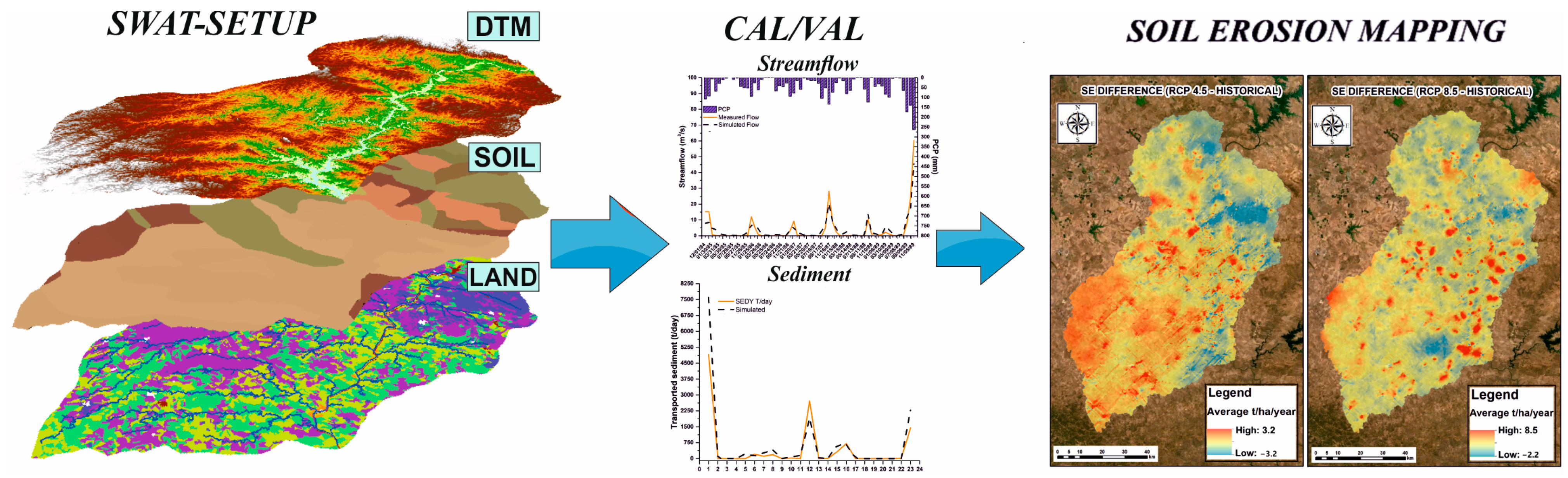
2.4. Modeling Framework

The main step of the SWAT model consists in the creation of hydrological response units (HRUs), which refer to all those parts of an area characterized by a unique combination of land use, morphological, and soil characteristics [54]. All the model’s outputs, such as runoff, evapotranspiration, aquifer recharge, sediment, and nutrient loadings from each HRU, are obtained and further summarized to obtain the sub-basin loading. The SWAT models calculate the outputs of runoff and sediment yield using a modified version of the curve number method [21,55] or the Green–Ampt infiltration method and the modified universal soil loss equation (MUSLE) [56], respectively. The ArcSWAT interface on ArcGIS 10.2 was used to develop the SWAT model for the Guadiana sub-basin.

2.4.1. SWAT Setup

All the physical characteristics, such as morphology, land cover, and soil properties, were evaluated and used as main inputs to build the SWAT model and to define the spatial distribution of the HRUs in the whole basin (Figure 3). An area of 37,233 km2 was divided into 99 sub-basins, which were further discretized into 3000 HRUs, using the automatic watershed delineation tool. Five slope classes (<5, 5–10, 10–15, 15–20, >20), seven land cover categories (Figure 2b), and six soil groups (Figure 2c) were identified and intersected. The CLC classification was reclassified to match with the vegetation cover types representative of the SWAT default database. Specifically, URMD was used to describe artificial settlements; OATS and OLIV for rainfed crops and olive plantations, respectively; FRSE for rainfed forest; and PINE for coniferous and mixed forest, while the “montado” system was represented using the SWAT code WPAS, which usually refers to winter pasture cover, specifically modified to account the characteristics of the montado system (30% OAK and 70% PAST) since the montado cover is not accounted in the SWAT default database. Some parameters characterizing the typical Mediterranean vegetation were updated according to Nùnes et al. [42]. Concerning the soils’ properties, all the information about Ks, AWC, texture, soil organic carbon (SOC), BD, and soil albedo utilized for the simulation is resumed in Table S1. Meteorological data were obtained from the database “Iberia01”, while actual evapotranspiration (AET) was calculated via the Hargreaves formula [57]. Specifically, SWAT uses the value of rain gauges to obtain the rainfall distribution according to the orographic characteristics of the basin and the density and proximity of the available stations.

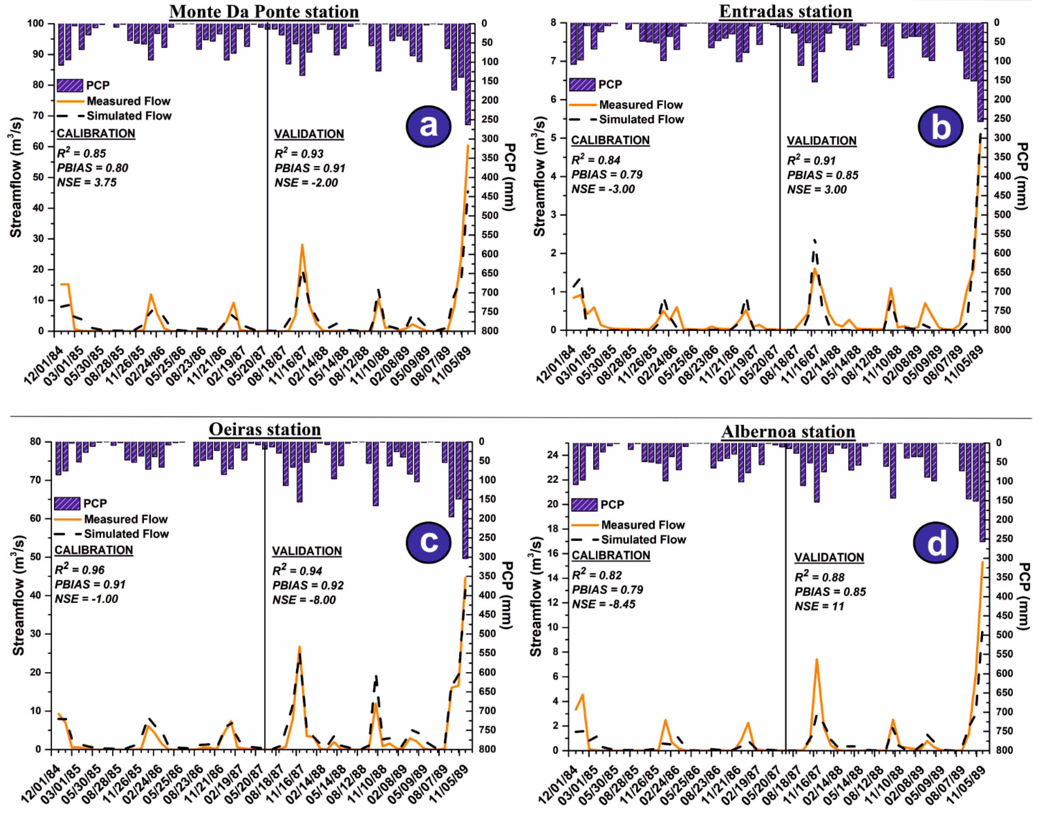
2.4.2. Calibration/Validation

After the setup procedure, the monthly SWAT simulation was divided into three blocks: (i) a warm-up period of 4 years (1980–1984), (ii) a calibration phase from January 1985 to June 1987, and (iii) a validation phase for the period July 1987–December 1989. For SE, only two hydrometric stations (Monte da Ponte and Oeiras) were available with scattered daily data for the period 1984–1989. A total of 38 daily SE datasets were available, which were evenly distributed to carry out the calibration and validation analysis. Finally, the SWAT model was used to simulate the historical period (1980–2000) and the future period (2020–2040) with the selected RCM (KNMI) under two different emission pathways (RCP 4.5 and 8.5). An extensive calibration/validation procedure was used to assess the robustness of the methodology. A preliminary “trial-and-error calibration” and an “automated calibration and validation” were performed. In the trial-and-error calibration, the fitted values of some parameters, such as groundwater “revap” coefficient (GW_REVAP), deep aquifer percolation fraction (RCHGDP), soil evaporation factor (ESCO), and plant uptake compensation (EPCO), were manually adjusted considering the results obtained by Nùnes et al. [58], who performed a SWAT application in a nearby catchment. The standalone software SWAT-CUP via the Sequential Uncertainty Fitting version 2 (SUFI-2) algorithm [59] was used for the auto calibration/validation. A total of three thousand calibration runs, divided in six interactions of five hundred runs each, were performed until a satisfactory calibration was obtained according to the thresholds suggested by Moriasi et al. [60] and calculating three statistical indices (Table 1): (i) the coefficient of determination (R2), (ii) the Nash–Sutcliffe efficiency (NSE), and (iii) the percent of bias (PBIAS), while the P-factor and R-factor values were investigated to account for model fit and uncertainties [61].

2.4.3. Soil Erosion Mapping

The values of SE in t/ha/year were obtained for the whole watershed in each HRU for the three analyzed scenarios. Thereafter, these values were averaged for 20 years and then spatialized using kriging techniques. Finally, the obtained maps were classified to produce three SE susceptibility maps and two spatial differences so as to highlight the main changes over time and to identify those areas where SE will increase/decrease in the future with relative uncertainties (Figure 3).

3. Results

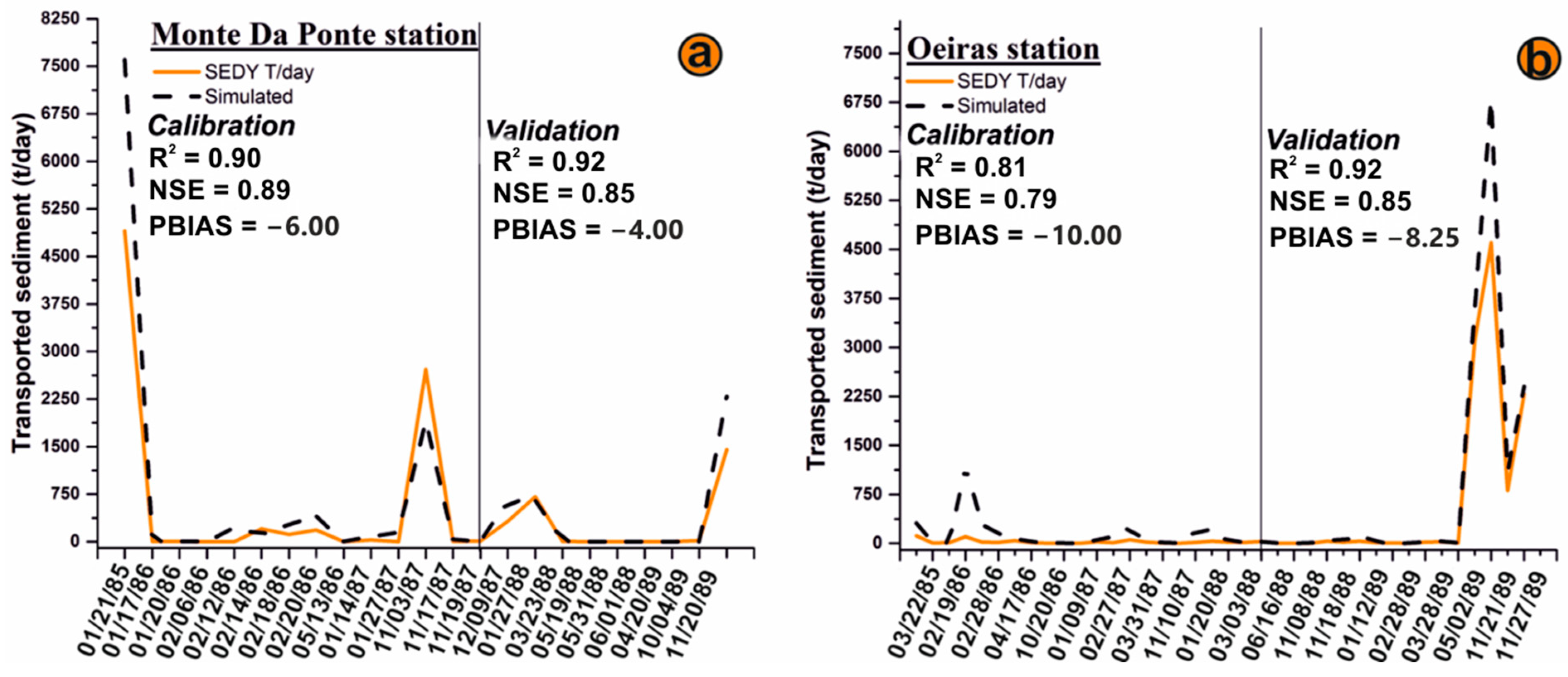
3.1. SWAT Calibration and Validation

The SWAT model successfully simulated both the streamflow and sediment regime of the watershed (Figure 4 and Figure 5). For the streamflow, the calibration results showed a very good agreement between simulated and observed data, with high R2, NSE, and good PBIAS in all available hydrometric stations (Figure 4). Similarly, the statistical indices for the validation procedure were within the range of a “very good” model performance according to the model’s performance criteria established by Moriasi et al. [60] (Table 1). Considering the sediment load calibration, despite using randomly distributed sediment data, simulated and observed data showed a “very good” performance match for calibration and validation in both the Monte Da Ponte (Figure 5a) and Oeiras (Figure 5b) stations. Regarding the streamflow simulation, the calibration/validation phases showed more than 70% of data bracketed by 95PPU (P-factor ≥ 0.70) with R-factors ranging from 0.15 to 0.3. For sediment, both Monte da Ponte and Oeiras reached a P-factor ≥ 0.6 with an R-factor of 0.32 and 0.41, respectively. All parameters responsible for streamflow and sediment loading, used to calibrate the model, were identified through an extensive literature review [62,63,64], and are reported in Table 2.
A global sensitivity analysis was implemented to identify those parameters that strongly influenced the simulated flow and soil losses within those listed in Table 2. The significance of the sensitivity test was evaluated using the statistical index “p-value”, automatically generated through the application of the SUFI-2 algorithm. The results of the sensitivity analysis (Table 2, where the bold parameters represent the sensitive ones) indicated that the streamflow simulation was strongly dependent on DEEP_IMP, GW_DELAY, RCHGR_DP, and ALPHA_BF, while SLSUBBSN, USLE_K, and USCLE_C were the main parameters influencing the sediment loss simulation.

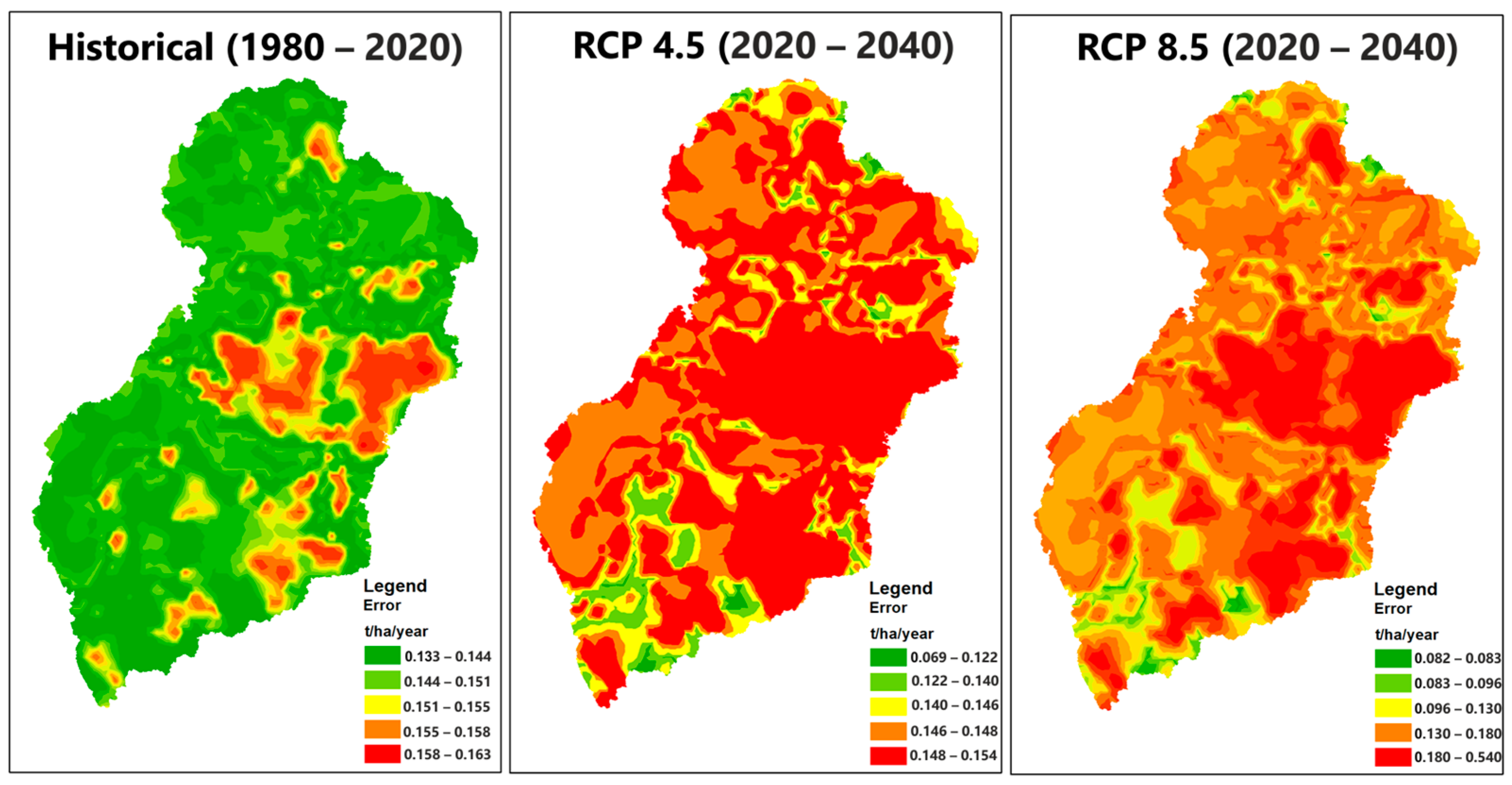
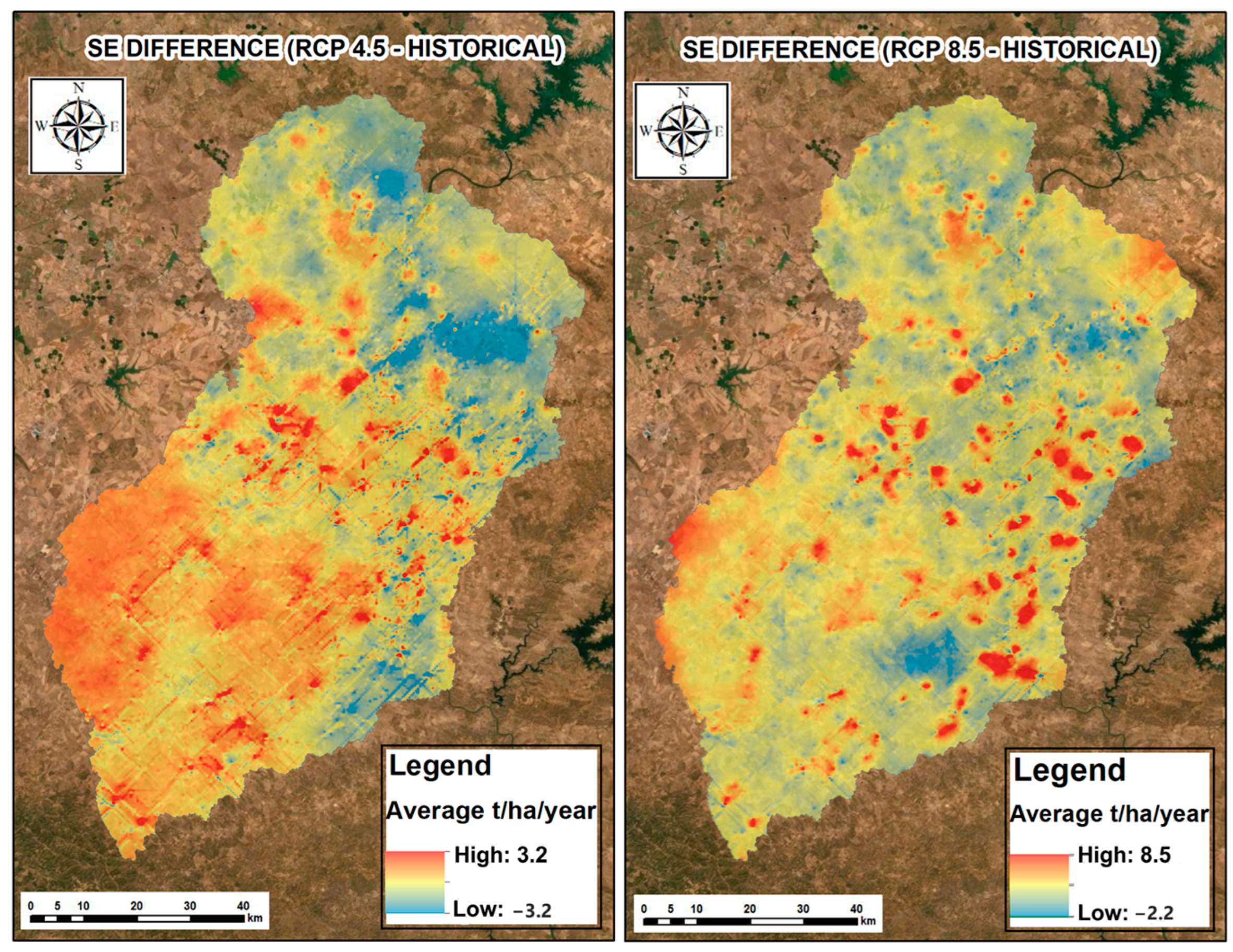
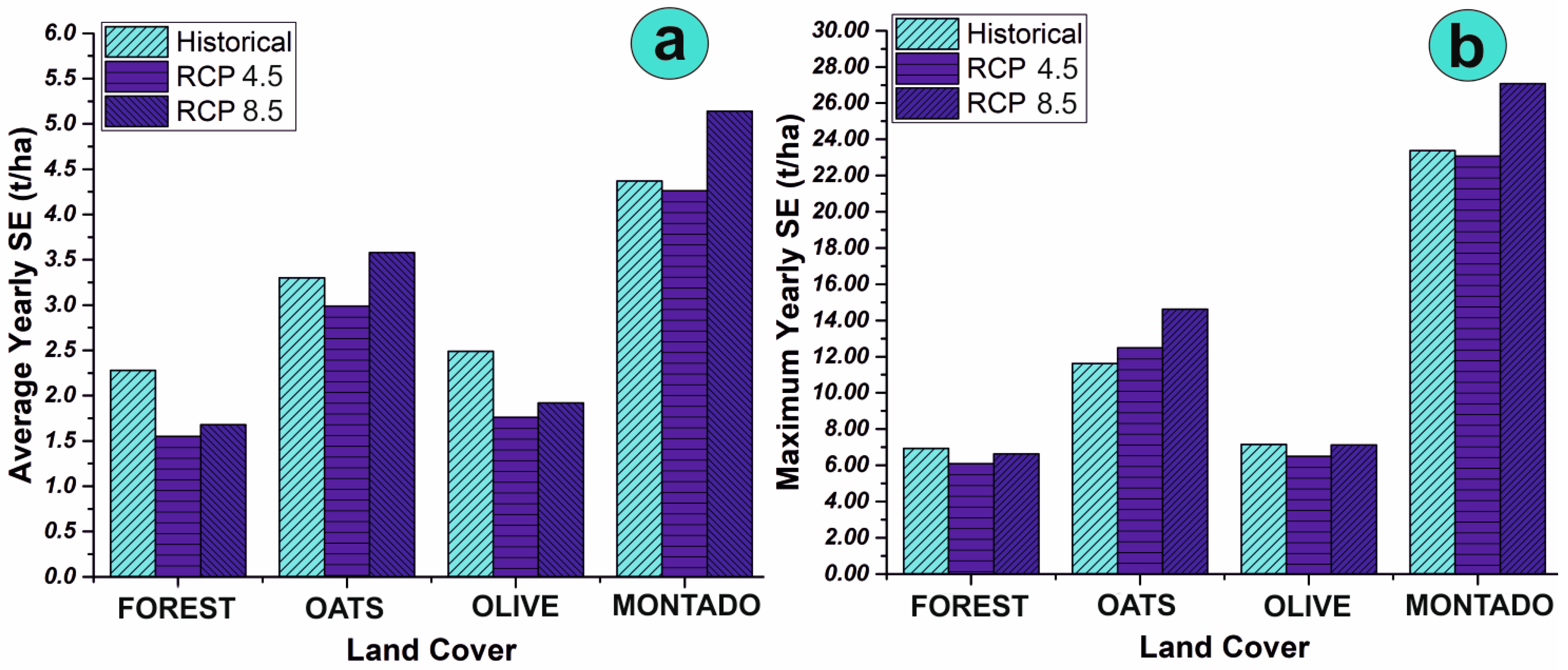
3.2. Estimated Soil Erosion Rates under Climate Scenarios

The simulated SE rates were averaged for the whole watershed over a period of 20 years, providing values of 3.3, 2.9, and 3.0 t/ha/year for the HIST, RCP 4.5, and RCP 8.5 scenarios, respectively. Maximum SE rates were also estimated, providing values of 25.3, 23.1, and 26.1 t/ha/year for the HIST, RCP 4.5, and RCP 8.5 scenarios, respectively. The average value of SE for HIST, RCP 4.5, and RCP 8.5 in each HRU was instead used as a single-point estimate to obtain a spatial distribution of the SE phenomenon over the entire basin, applying the kriging interpolation method. The spatialized data were grouped in five classes of SE susceptibility following the classification proposed by Panagos et al. [65]: very low (SE ≤ 1.0 t/ha/year), low (1.0 < SE ≤ 2.5 t/ha/year), medium (2.5 < SE ≤ 4.0 t/ha/year), high (4.0 < SE ≤ 5.5 t/ha/year), and very high (SE > 5.5 t/ha/year). The susceptibility maps of the basin are showed in Figure 6. The SE susceptibility of the area during the reference period (HIST) shows the highest values in the central and southern parts of the study site, while the lowest values are estimated for the eastern border of the basin and in the northern area (Figure 6a). In future conditions (RCP 4.5 in Figure 6b and RCP 8.5 in Figure 6c), the distribution of the SE susceptibility remains similar to the one of the HIST scenario in terms of spatial distribution of the zones most prone to SE risk (Figure 5a). The uncertainty maps shown in Figure 7 present overall low errors, which increase in an absolute value moving from HIST < RCP 4.5 < RCP 8.5. In all cases, the portions of the basins most susceptible to SE are in correspondence to Leptosols, followed by Vertisols and Luvisols (Figure 2c). The most interesting results were observed by calculating the patterns of SE change between the future projections (RCP 4.5 and 8.5) and the HIST scenario (Figure 8), obtained using a spatial difference through a raster calculator in a GIS environment.
The HIST-RCP 4.5 map shows a wider presence of areas characterized by an increase in absolute value of SE (t/ha/year) compared with HIST-RCP 8.5, especially in the south-west portion of the basin. On the other hand, the HIST-RCP 8.5 map shows that under this extreme climatic scenario, there will be an increase in hotspots with high SE rates, probably because of the concentration of extreme rainfall events, while most of the basin will not experience big changes in SE susceptibility. Using the land cover variables as aggregation criterion, the SE values of the HRUs were averaged to homogenize soil (Vertisols, Luvisols, and Leptosols) and slope characteristics. According to the area characteristics, four main land covers were selected as the most representative of the basin, since together they occupy more than 95% of the entire territory: (i) oats plantation (OATS), (ii) evergreen forest (FRSE), (iii) olive plantation (OLIV), and (iv) the agroforestry system “montado” (WPAS). Figure 9 shows the 20 years’ average (Figure 9a) and 20 years’ maximum SE in t/ha/year (Figure 9b) for each land cover. Results highlight that the SE rate is in the order FRSE < OLIV < OATS < WPAS for both average and maximum values. Table 3 clearly shows that in the projected climatic scenario RCP 4.5, all land covers will slightly decrease their SE rates. Conversely, the extreme scenario RCP 8.5 would not change the SE rates in the areas with FRSE and OLIV but would slightly worsen the SE rates for the soils under OATS and WPAS, reaching SE rates even higher than the ones modeled for HIST.

4. Discussion

4.1. Projected Soil Erosion Rates

The projected changes in SE rates with a BAU scenario under the future climatic conditions provided an average yearly SE rate for the next 20 years in the order of 2.9 and 3.0 t/ha/year for RCPs 4.5 and 8.5, respectively, both slightly lower than the HIST (1980–2000) average of 3.3 t/ha/year. The results agree with the projected climate indices for the area, which depict a future scenario of lowering precipitation and moderate extremes’ increment. HIST and future values of SE were comparable with the SE classification proposed by Panagos et al. [1] for the Alentejo region, which reported SE rates from 2.0 to 5.0 t/ha/year, but they are higher than the estimated average SE rate of 1.2 t/ha/year reported by Cerdan et al. [21] for the whole area of Portugal. In terms of soil stability and sustainability, a tolerable range of SE between 0.3 and 1.4 t/ha/year is recommended to maintain a sustainable equilibrium between soil formation and soil loss for the European countries [66]. Both HIST and future SE rates estimated in our sites are higher than this proposed tolerable range, but they agree with the results reported by Panagos et al. [65], which forecasted an average SE for 2050 equal to 3.7 t/ha/year in agricultural areas across Europe. Moreover, the concomitant occurrence of dry and wet extremes due to CC might exacerbate the susceptibility to desertification of the entire region, increasing SE, decreasing crop yields, and decreasing livestock productivity, with cascading effects on food security and nutrition [67]. Such SE rates represent a serious environmental issue for the driest areas of Europe, such as the Alentejo, under agricultural land use. The SE results obtained in the simulation for the whole basin showed an improving SE trend, under the RCP 4.5 scenario (Table 3), with values that remained below 2 t/ha/year for FRSE and OLIV, which together cover 33% of the studied basin. However, the SE data reported in Table 2 are the average of land units characterized by the same land cover but having different parameters relevant for SE rate magnitude, such as slope, soil type, and other soil physical characteristics [68].

4.2. Soil Erosion Susceptibility Maps

To improve land management, it is more effective to represent the results in terms of SE susceptibility maps, rather than representing them as a simple average of the analyzed SE for the whole basin whose areas might be more susceptible to the further increment of SE risk in the future. These maps showed a comparable pattern of the susceptibility classes for the HIST and the future scenarios (RCP 4.5 and 8.5) (Figure 6). On the other hand, comparing the maps of the SE difference between the HYST and the two future scenarios (Figure 8), a very different average SE pattern is evident, which might be very relevant for management purposes. The yearly SE average will be lower compared with the HIST scenario, with few exceptions mainly located in the central area of the basin.

4.3. Factors Affecting SE

Considering the RCP 4.5 scenario, 95% of the most endangered areas are characterized by Leptosols, slope > 10%, and a predominant land cover of managed ecosystems (WPAS 50%, OAT 25%, OLIV 2%). Such a combination of factors makes these areas particularly in need of a dedicated land management plan to reduce SE impacts. In this study, the SE susceptibility was more strongly influenced by soil and land use rather than morphology. In fact, the concomitant presence of WPAS on Leptosols determined the highest SE susceptibility of the whole central southern part of the basin [41,42]. On the one hand, Leptosols’ peculiarities (i.e., sandy texture, low soil’s depth, and low SOC) [69] negatively impact soil erodibility, (i) hindering vegetation development [70] that affects SOC content that and in turn contributes to soil aggregates formation [71] and (ii) saturating itself faster during rainfall, thus accelerating the beginning of runoff [72]. On the other hand, the presence of the montado system (WAPS) characterized by the exploitation of multiple resources (i.e., livestock, forestry, and crops) causes severe impacts on soil, increasing SE risk despite the presence of forestry and olive plantations. Moreover, grazing activities, common in the montado system, can further reduce the vegetation cover that in turn negatively affects surface runoff under different rainfall intensity events, promoting soil loss. Schnabel et al. [73] showed that for the grazed “dehesa” systems of Extremadura, an environmental system like “montando”, a ground cover of at least 60% was necessary to protect the soil during exceptionally high-intensity storms (I-30 > 40 mm·h−1). Meanwhile, a ground cover lower than 20% represented a threat, because soil loss occurred even in moderately intense storms. Mean SE rates related to sheet wash events were estimated to vary between 0.12 and 1.34 t/ha/year for 60% and 20% of ground cover, respectively. These estimates, corroborated by the studies of Kosmas et al. [74] and Ceballos et al. [75], clearly highlighted the key role of vegetation in land surface processes, which is why vegetation can be considered an ecosystem service provider [76]. Finally, the low SE susceptibility across the northeastern border of the watershed matches the OLIV (medium to low SE) and FRSE (low SE) distribution on soil formations other than Leptosols. Regarding the other two main soil groups, Vertisols exhibited a higher average erosion rate than Luvisols in both RCP 4.5 and 8.5. Vertisol tends to be highly erodible because of its huge clay content that entails a strong aggregation. This means that Vertisols erode largely as aggregated material, resulting in high rates of sediments transported. In addition, Vertisols showed a low infiltration rate when wet, which results in an increase in surface runoff [77]. Considering the results, Vertisols erode less then Leptosols (median of 2.25 t/ha/years compared with 4.03 t/ha/year) but more than Luvisols (1.91 t/ha/year). In all cases, “montado” is the most susceptible land cover to SE, followed by oats and olive plantations, while forests (FRSE) proved to exert a protective action on soil [78], exhibiting the lowest SE rates due to their capacity to intercept the rainfall by the tree canopies, independently of the soil type and morphology that characterize the area.

4.4. Soil Erosion Susceptibility Management

The average SE rate calculated for the whole basin can be considered a relevant reference value for the planning of future management strategies for soil and water conservation [79]. The effectiveness of these strategies may vary, depending on the specific characteristics of the land, climate, and local regulations. Anyway, the combination of proper conservation practices with a concise education and awareness of the local farmer becomes mandatory to achieve a soil erosion mitigation. Likewise, the SE susceptibility maps, by identifying which areas might be more susceptible to further SE increment, can be an important tool for policy makers and farmers for watershed management. This assumption has been proved in several studies across India [6], Italy [80], Morocco [81], and Ethiopia [82]. According to the obtained results, several sustainable land management (SLM) practices could be tested and adopted to counter the increasing SE. Naturalization should be preferred to agricultural management and deforestation, especially on Leptosols, and this would be relevant even at a relatively low slope [83]. Permanent crops with greening management should be preferred to seasonal crops in areas under predominant agricultural management [84]. With special reference to olive farming in Mediterranean regions, SE represents the principal environmental problem [85], and both no-tillage soil management and cover crop development are proposed as adaptation strategies to CC impacts [86]. Overgrazing should be carefully avoided [87], introducing a holistic planned grazing [88] to promote grassland self-regeneration. To make such an assessment effective in the long term, a projection of future SE risk is extremely useful for the protection and management of watersheds. However, although the highest SE values were found for the RCP 8.5 scenario, which is the least likely of the two, in the light of EU policies in support of climate change mitigation and sustainable development (e.g., Green Deal, Farm to Fork strategies, etc.), awareness raising among managers and landowners is suggested. Another relevant issue to consider is the significance of the estimated SE rates in terms of desertification and soil degradation risk, comparing the magnitude of SE rates with soil formation rates. Considering that the average 20-year values obtained from this study in all the time periods are higher than the desirable range of SE, compared with the rate of soil formation [66], the implementation of management plans aimed to improve land use and promote countermeasures to reduce SE becomes mandatory and urgent.

5. Conclusions

In this study, the SWAT model was successfully applied to a Mediterranean watershed in South Portugal, in areas at risk of desertification, to assess the impact of current land management on the rate of SE under current and future climate scenarios. The role of a combination of relevant factors in determining SE rates was assessed using SE susceptibility maps. Overall, our data highlight a very variable spatial distribution of areas at different SE risks under future climate scenarios, ranging from areas where SE will decrease compared with current climate conditions to areas where SE will continue to increase. The fact that most of these areas are currently under land management is a matter of immediate concern, proving the need for appropriate measures. This information could be of great help for awareness raising among farmers, livestock breeders, and landowners. The results also underlined that although climate change may exacerbate conditions in the most vulnerable areas, in several areas of the basin, current conditions are already above the recommended threshold for maintaining a sustainable balance between soil formation and soil loss, fostering the risk of desertification.

Supplementary Materials

The following supporting information can be downloaded at https://www.mdpi.com/article/10.3390/su151712992/s1: Figure S1: Thermo-pluviometric diagram for the Alentejo region; Table S1: Morphology slope and land cover classification (CLC, 2018) for the four study sites; Table S2: SWAT soil parameters for the identified soil groups.

Author Contributions

Conceptualization: G.B., M.M. and S.C.; methodology: G.B.; software: G.B. and S.C.P.C.; validation: G.B., E.G. and M.M.; investigation: G.B. and E.G.; resources: S.C.; data curation: G.B., E.G. and S.C.P.C.; writing—original draft preparation: G.B.; writing—review and editing: M.M. and S.C.; supervision: S.C. All authors have read and agreed to the published version of the manuscript.

Funding

The present study is supported by the EU project LIFE16 CCA/IT/000011.

Institutional Review Board Statement

Not Applicable.

Informed Consent Statement

Not Applicable.

Data Availability Statement

All data used for this work are available at the author’s request.

Acknowledgments

We thank the Associaçao de Defesa do Patrimonio de Mértola for supporting during the field sampling. We also want to thank Joao Pedro Nùnes for assisting in the preliminary model setup.

Conflicts of Interest

The authors declare no conflict of interest.

References

  1. Panagos, P.; Borrelli, P.; Meusburger, K.; Alewell, C.; Lugato, E.; Montanarella, L. Estimating the soil erosion cover-management factor at the European scale. Land Use Policy 2015, 48, 38–50. [Google Scholar] [CrossRef]
  2. Adhikari, K.; Hartemink, A.E. Linking soils to ecosystem services—A global review. Geoderma 2016, 262, 101–111. [Google Scholar] [CrossRef]
  3. Grilli, E.; Carvalho, S.C.P.; Chiti, T.; Coppola, E.; D’Ascoli, R.; La Mantia, T.; Marzaioli, R.; Mastrocicco, M.; Pulido, F.; Rutigliano, F.A.; et al. Critical range of soil organic carbon in southern europe lands under desertification risk. J. Environ. Manag. 2021, 287, 112285. [Google Scholar] [CrossRef] [PubMed]
  4. Zhao, G.; Mu, X.; Wen, Z.; Wang, F.; Gao, P. Soil erosion, conservation, and eco-environment changes in the loess plateau of China. Land Degrad. Dev. 2013, 24, 499–510. [Google Scholar] [CrossRef]
  5. Arabameri, A.; Pradhan, B.; Pourghasemi, H.R.; Rezaei, K. Identification of erosion prone areas using different multi-criteria decision-making techniques and GIS. Geomat. Nat. Hazards Risk 2018, 9, 1129–1155. [Google Scholar] [CrossRef]
  6. Bhattacharya, R.K.; Chatterjee, N.D.; Das, K. Sub-basin prioritization for assessment of soil erosion susceptibility in Kangsabati, a plateau basin: A comparison between MCDM and SWAT models. Sci. Total Environ. 2020, 734, 139474. [Google Scholar] [CrossRef]
  7. Borrelli, P.; Robinson, D.A.; Panagos, P.; Lugato, E.; Yang, J.E.; Alewell, C.; Wupper, D.; Montanarella, L.; Ballabio, C. Land use and CC impacts on global soil erosion by water (2015–2070). Proc. Natl. Acad. Sci. USA 2020, 117, 21994–22001. [Google Scholar] [CrossRef] [PubMed]
  8. Burt, T.; Boardman, J.; Foster, I.; Howden, N. More rain, less soil: Long-term changes in rainfall intensity with climate change. Earth Surf. Process. Landf. 2016, 41, 563–566. [Google Scholar] [CrossRef]
  9. Yang, D.; Kanae, S.; Oki, T.; Koike, T.; Musiake, K. Global potential soil erosion with reference to land use and climate changes. Hydrol. Process. 2003, 17, 2913–2928. [Google Scholar] [CrossRef]
  10. IPCC: Intergovernmental Panel on Climate Change. Climate Change 2014: Synthesis Report. Contribution of Working Groups I, II and II to the Fifth Assessment Report of the Intergovernmental Panel on Climate Change; IPCC: Geneva, Switzerland, 2014; p. 151. [Google Scholar]
  11. Giorgi, F. Climate change hot-spots. Geophys. Res. Lett. 2006, 33, L08707. [Google Scholar] [CrossRef]
  12. Giorgi, F.; Lionello, P. Climate change projections for the Mediterranean region. Glob. Planet Chang. 2008, 63, 90–104. [Google Scholar] [CrossRef]
  13. Zittis, G.; Hadjinicolaou, P.; Klangidou, M.; Proestos, Y.; Lelieveld, J. A multi-model, multi-scenario, and multi-domain analysis of regional climate projections for the Mediterranean. Reg. Environ. Chang. 2019, 19, 192621–192635. [Google Scholar] [CrossRef]
  14. Moriondo, M.; Good, P.; Durao, R.; Bindi, M.; Giannakopoulos, C.; Corte-Real, J. Potential impact of climate change on fire risk in the Mediterranean area. Clim. Res. 2006, 31, 85–95. [Google Scholar] [CrossRef]
  15. Busico, G.; Giuditta, E.; Kazakis, N.; Colombani, N. A hybrid GIS and AHP approach for modelling actual and future forest fire risk under climate change accounting water resources attenuation role. Sustainability 2019, 11, 7166. [Google Scholar] [CrossRef]
  16. Raclot, D.; Le Bissonnais, Y.; Annabi, M.; Sabir, M. Sub-chapter 2.3.3. Challenges for Mitigating Mediterranean Soil Erosion under Global Change. In The Mediterranean Region under Climate Change; IRD Éditions: Marseille, France, 2016; ISBN 9782709922203. [Google Scholar]
  17. Samela, C.; Imbrenda, V.; Coluzzi, R.; Pace, L.; Simoniello, T.; Lanfredi, M. Multi-Decadal Assessment of Soil Loss in a Mediterranean Region Characterized by Contrasting Local Climates. Land 2022, 11, 1010. [Google Scholar] [CrossRef]
  18. Borrelli, P.; Robinson, D.A.; Fleischer, L.R.; Lugato, E.; Ballabio, C.; Alewell, C.; Meusburger, K.; Modugno, S.; Schütt, B.; Ferro, V.; et al. An Assessment of the Global Impact of 21st Century Land Use Change on Soil Erosion. Nat. Commun. 2017, 8, 2013. [Google Scholar] [CrossRef]
  19. Wischmeier, W.H.; Smith, D.D. Predicting Rainfall Erosion Losses—A Guide for Conservation Planning; U.S. Department of Agriculture, Agriculture Handbook: Annapolis, ML, USA, 1978; p. 537.
  20. Renard, K.G.; Foster, G.R.; Weesies, G.A.; McCool, D.K.; Yoder, D.C. Predicting Soil Erosion by Water: A Guide to Conservation Planning with the Revised Universal Soil Loss Equation (RUSLE); United States Department of Agriculture, Agricultural Research Service (USDA-ARS) Handbook 703; United States Government Printing Office: Washington, DC, USA, 1997.
  21. Cerdan, O.; Govers, G.; Le Bissonnais, Y.; Van Oost, K.; Poesen, J.; Saby, N.; Gobin, A.; Vacca, A.; Quinton, J.; Auerswald, K.; et al. Rates and spatial variations of soil erosion in Europe: A study based on erosion plot data. Geomorphology 2010, 122, 167–177. [Google Scholar] [CrossRef]
  22. Maltsev, K.; Yermolaev, O. Assessment of soil loss by water erosion in small river basins in Russia. Catena 2020, 195, 104726. [Google Scholar] [CrossRef]
  23. Brakensiek, D.L.; Rawls, W.J.; Stephenson, G.R. Modifying SCS Hydrologic Soil Groups and Curve Numbers for Rangeland Soils; ASAE Paper No. PNR-84–203; American Society of Agricultural Engineers: St. Joseph, MI, USA, 1934. [Google Scholar]
  24. Panagos, P.; Borrelli, P.; Poesen, J.; Ballabio, C.; Lugato, E.; Meusburger, K.; Montanarella, L.; Alewell, C. The new assessment of soil loss by water erosion in Europe. Environ. Sci. Pol. 2015, 54, 438–447. [Google Scholar] [CrossRef]
  25. Alewell, C.; Borrelli, P.; Meusburger, K.; Panagos, P. Using the USLE: Chances, challenges, and limitations of soil erosion modelling. ISWCR 2019, 7, 203–225. [Google Scholar] [CrossRef]
  26. Laflen, J.M.; Elliot, W.J.; Flanagan, D.C.; Meyer, C.R.; Nearing, M.A. WEPP-predicting water erosion using a process-based model. J. Soil Water Conserv. 1997, 52, 96–102. [Google Scholar]
  27. De Roo, A.P.J.; Wesseling, C.G.; Ritsema, C.J. Lisem: A single-event physically based hydrological and soil erosion model for drainage basins. I: Theory, input and output. Hydrol. Process. 1997, 10, 1107–1117. [Google Scholar] [CrossRef]
  28. Arnold, J.G.; Moriasi, D.N.; Gassman, P.W.; Abbaspour, K.C.; White, M.J.; Srinivasan, R.; Santhi, C.R.; Harmel, D.; van Griensven, A.; Van Liew, M.W.; et al. SWAT: Model Use, Calibration, and Validation. Trans. ASABE 2012, 55, 1491–1508. [Google Scholar] [CrossRef]
  29. Morgan, R.P.C.; Quinton, J.N.; Smith, R.E.; Govers, G.; Poesen, J.W.A.; Auerswald, K.; Chisci, G.; Torri, D.; Styczen, M.E. The European soil erosion model (EUROSEM): A dynamic approach for predicting sediment transport from fields and small catchments. Earth Surf. Process. Landf. 1998, 23, 527–544. [Google Scholar] [CrossRef]
  30. Arnold, J.G.; Srinivasan, R.; Muttiah, R.S.; Williams, J.R. Large-area hydrologic modeling and assessment: Part I. Model development. J. Am. Water Resour. Assoc. 1998, 34, 73–89. [Google Scholar] [CrossRef]
  31. Bhatta, B.; Shrestha, S.; Shrestha, P.K.; Talchabhadel, R. Evaluation and application of a SWAT model to assess the CC impact on the hydrology of the Himalayan River basin. Catena 2019, 181, 104082. [Google Scholar] [CrossRef]
  32. Busico, G.; Colombani, N.; Fronzi, D.; Pellegrini, M.; Tazioli, A.; Mastrocicco, M. Evaluating SWAT model performance, considering different soils data input, to quantify actual and future runoff susceptibility in a highly urbanized basin. J. Environ. Manag. 2020, 266, 110625. [Google Scholar] [CrossRef]
  33. Busico, G.; Ntona, M.M.; Carvalho, S.C.P.; Patrikaki, O.; Voudouris, K.; Kazakis, N. Simulating future groundwater recharge in coastal and inland catchments. Water Resour. Manag. 2021, 35, 3617–3632. [Google Scholar] [CrossRef]
  34. Tasdighi, A.; Arabi, M.; Harmel, D. A probabilistic appraisal of rainfall-runoff modeling approaches within SWAT in mixed land use watersheds. J. Hydrol. 2018, 564, 476–489. [Google Scholar] [CrossRef]
  35. Golmohammadi, G.; Rudra, R.; Dickinson, T.; Goel, P.; Veliz, M. Predicting the temporal variation of flow contributing areas using SWAT. J. Hydrol. 2017, 54, 375–386. [Google Scholar] [CrossRef]
  36. Abbaspour, K.C.; Vaghefi, S.A.; Yang, H.; Srinivasan, R. Global soil, land-use, evapotranspiration, historical and future weather databases for SWAT Applications. Sci. Data 2019, 6, 263. [Google Scholar] [CrossRef]
  37. Chambel, A.; Duque, J.; Nascimento, J. Regional Study of Hard Rock Aquifers in Alentejo, South Portugal: Methodology and Results. In IAH-SP Series; Krásný, J., Sharp, J.M., Eds.; Taylor and Francis: Oxfordshire, UK, 2007; pp. 73–93. [Google Scholar]
  38. Beck, H.E.; Zimmermann, N.E.; McVicar, T.R.; Vergopolan, N.; Berg, A.; Wood, E.F. Present and future köppen-geiger climate classification maps at 1-km resolution. Sci. Data 2018, 5, 180–214. [Google Scholar] [CrossRef] [PubMed]
  39. Ramos, C.; Reis, E. As cheias no sul de Portugal em diferentes tipos de bacias hidrográficas. Finisterra 2001, 36, 61–82. [Google Scholar] [CrossRef]
  40. USS Working Group WRB. World Reference Base for Soil Resources 2014, Update 2015 International Soil Classification System for Naming Soils and Creating Legends for Soil Maps. In World Soil Resources Reports No. 106; FAO: Rome, Italy, 2015. [Google Scholar]
  41. Pinto-Correia, T.; Mascarenhas, J. Contribution to the extensification/intensification debate: New trends in the Portuguese montado. Landsc. Urban Plan 1999, 46, 125–131. [Google Scholar] [CrossRef]
  42. Nùnes, J.P.; Seixas, J.; Pacheco, N.R. Vulnerability of water resources, vegetation productivity and soil erosion to CC in Mediterranean watersheds. Hydrol. Process. 2008, 22, 3115–3134. [Google Scholar] [CrossRef]
  43. Roxo, M.J.; Casimiro, P.C. Long Term Monitoring of Soil Erosion by Water, Vale Formoso Erosion Centre—Portugal’. Soil Conservation and Protection for Europe Project. Available online: http://eusoils.jrc.ec.europa.eu/projects/scape/uploads/97/Roxo_Casimiro.pdf (accessed on 12 April 2022).
  44. FAO: Food and Agriculture Organization of the United Nations. 2007. Available online: https://land.copernicus.eu/pan-european/corine-land-cover (accessed on 14 January 2020).
  45. DGADR: Direcção-Geral de Agricultura e Desenvolvimento Rural. Solos, Cartografiaeinformação Geográfia; DGADR: Lisboa, Portugal, 2013.
  46. Batjes, N.H.; Ribeiro, E.; van Oostrum, A. Standardised soil profile data to support global mapping and modelling (WoSIS snapshot 2019). Earth Syst. Sci. Data 2020, 12, 299–320. [Google Scholar] [CrossRef]
  47. Batjes, N.H.; Ribeiro, E.; van Oostrum, A.; Leenaars, J.; Hengl, T.; Mendes de Jesus, J. WoSIS: Providing standardized soil profile data for the world. Earth Syst. Sci. Data 2017, 9, 1–14. [Google Scholar] [CrossRef]
  48. Ribeiro, E.; Batjes, N.H.; van Oostrum, A.J.M. World Soil Information Service (WoSIS)—Towards the Standardization and Harmonization of World Soil Data: Procedures Manual ISRIC Report 2020/01; ISRIC—World Soil Information: Wageningen, The Netherlands, 2020; p. 166. [Google Scholar]
  49. SNIRH: Sistema Nacional de Informação de Recursos Hídricos. 2006. Available online: https://snirh.apambiente.pt/ (accessed on 23 November 2019).
  50. Herrera, S.; Fernandez, J.; Gutierrez, J.M. Update of the Spain02 Gridded Observational Dataset for Euro-CORDEX evaluation: Assessing the Effect of the Interpolation Methodology. Int. J. Climatol. 2016, 36, 900–908. [Google Scholar] [CrossRef]
  51. Herrera, S.; Gutierrez, J.M.; Ancell, R.; Pons, M.R.; Frias, M.D.; Fernandez, J. Development and analysis of a 50-year high-resolution daily gridded precipitation dataset over Spain (Spain02). Int. J. Climatol. 2012, 32, 74–85. [Google Scholar] [CrossRef]
  52. Herrera, S.; Margarida Cardoso, R.; Matos Soares, P.; Espírito-Santo, F.; Viterbo, P.; Gutiérrez, J.M. Iberia01: A new gridded dataset of daily precipitation and temperatures over Iberia. Earth Syst. Sci. Data 2019, 11, 1947–1956. [Google Scholar] [CrossRef]
  53. Soares, P.M.; Cardoso, R.M.; Lima, D.C.; Miranda, P.M. Future precipitation in Portugal: High-resolution projections using WRF model and EURO-CORDEX multi-model ensembles. Clim. Dynam. 2017, 49, 2503–2530. [Google Scholar] [CrossRef]
  54. Neitsch, S.; Arnold, J.; Kiniry, J.; Williams, J. Soil and Water Assessment Tool Theoretical Documentation 2000; Grassland, Soil and Water Research Laboratory, Agricultural Research Service: Temple, TX, USA, 2000.
  55. USDA: United States Department of Agriculture. National Engineering Handbook, Part 630—Hydrology, Chapter 9: Hydrologic Soil-Cover Complexes 2004; USDA: Washington, DC, USA, 2004.
  56. Williams, J.R. Chapter 25: The EPIC Model. In Computer Models of Watershed Hydrology; Singh, V.P., Ed.; Water Resources Publications: Highlands Ranch, CO, USA, 1995; pp. 909–1000. [Google Scholar]
  57. Aschonitis, V.G.; Papamichail, D.; Demertzi, K.; Colombani, N.; Mastrocicco, M.; Ghirardini, A.; Castaldelli, G.; Fano, E.A. High-resolution global grids of revised Priestley–Taylor and Hargreaves–Samani coefficients for assessing ASCE standardized reference crop evapotranspiration and solar radiation. Earth Syst. Sci. Data 2017, 9, 615–638. [Google Scholar] [CrossRef]
  58. Nùnes, J.P.; Jacinto, R.; Keizer, J.J. Combined impacts of climate and socio-economic scenarios on irrigation water availability for a dry Mediterranean reservoir. Sci. Tot. Environ. 2017, 584–585, 219–233. [Google Scholar] [CrossRef]
  59. Abbaspour, K.C. SWAT-Calibration and Uncertainty Programs—A User Manual; Eawag—Swiss Federal Institute of Aquatic Science and Technology: Dübendorf, Switzerland, 2015; p. 103. [Google Scholar]
  60. Moriasi, D.; Arnold, J.; Van Liew, M.; Bingner, R.; Harmel, R.; Veith, T. Model evaluation guidelines for systematic quantification of accuracy in watershed simulations. Trans. ASABE 2007, 50, 885–900. [Google Scholar] [CrossRef]
  61. Abbaspour, K.C.; Johnson, A.; Van Genuchten, M.T. Estimating uncertain flow and transport parameters using a sequential uncertainty fitting procedure. Vadose Zone J. 2004, 3, 1340–1352. [Google Scholar] [CrossRef]
  62. Chen, Y.; Xu, C.-Y.; Chen, X.; Xu, Y.; Yin, Y.; Gao, L.; Liu, M. Uncertainty in simulation of land-use change impacts on catchment runoff with multi-timescales based on the comparison of the HSPF and SWAT models. J. Hydrol. 2019, 573, 486–500. [Google Scholar] [CrossRef]
  63. Khelifa, W.B.; Hermassi, T.; Strohmeier, S.; Zucca, C.; Ziadat, F.; Boufaroua, M.; Habaieb, H. Parameterization of the effect of bench terraces on runoff and sediment yield by swat modeling in a small semi-arid watershed in northern Tunisia. Land Degrad. Dev. 2017, 28, 1568–1578. [Google Scholar] [CrossRef]
  64. Serpa, D.; Nùnes, J.P.; Santos, J.; Sampaio, E.; Jacinto, R.; Veiga, S.; Lima, J.C.; Moreira, M.; Corte-Real, J.; Keizer, J.J.; et al. Impacts of climate and land use changes on the hydrological and erosion processes of two contrasting Mediterranean catchments. Sci. Total Environ. 2015, 538, 64–77. [Google Scholar] [CrossRef] [PubMed]
  65. Panagos, P.; Ballabio, C.; Himics, M.; Scarpa, S.; Matthews, F.; Bogonos, M.; Poesen, J.; Borrelli, P. Projections of soil loss by water erosion in Europe by 2050. Environ. Sci. Policy 2021, 124, 380–392. [Google Scholar] [CrossRef]
  66. Verheijen, F.G.A.; Jones, R.J.A.; Rickson, R.J.; Smith, C.J. Tolerable versus actual soil erosion rates in Europe. Earth Sci. Rev. 2019, 94, 23–38. [Google Scholar] [CrossRef]
  67. EEA—European Environment Agency. Climate Change Adaptation in the Agriculture Sector in Europe; EEA: Copenhagen, Denmark, 2019; p. 108.
  68. Dissanayake, D.; Morimoto, T.; Ranagalage, M. Accessing the soil erosion rate based on RUSLE model for sustainable land use management: A case study of the Kotmale watershed, Sri Lanka. Model Earth Syst. Environ. 2019, 5, 291–306. [Google Scholar] [CrossRef]
  69. Kosmas, C.; Gerontidis, S.; Marathianou, M. The effect of land use change on soils and vegetation over various lithological formations on Lesvos (Greece). Catena 2000, 40, 51–68. [Google Scholar] [CrossRef]
  70. Gabarrón-Galeote, M.A.; Martínez-Murillo, J.F.; Quesada, M.A.; Ruiz-Sinoga, J.D. Seasonal changes in the soil hydrological and erosive response depending on aspect, vegetation type and soil water repellency in different Mediterranean microenvironments. Solid Earth 2013, 4, 497–509. [Google Scholar] [CrossRef]
  71. Pedron, F.D.A.; Fink, J.R.; Rodrigues, M.F.; De Azevedo, A.C. Hydraulic conductivity and water retention in leptosols-regosols and saprolite derived from sandstone, Brazil. Rev. Bras. De Ciência Do Solo 2011, 35, 1253–1262. (In Portuguese) [Google Scholar] [CrossRef]
  72. Ebelhar, S.; Chesworth, W.; Paris, Q.; Spaargaren, O. Leptosols. In Encyclopedia of Soil Science; Encyclopedia of Earth Sciences Series; Chesworth, W., Ed.; Springer: Dordrecht, The Netherlands, 2008. [Google Scholar]
  73. Schnabel, S.; Dahlgren, R.A.; Moreno-Marcos, G. Soil and Water Dynamics. In Mediterranean Oak Woodland Working Landscapes; Cmpos, P., Huntsinger, L., Oviedo Pro, J.L., Starrs, P.F., Díaz, M., Standiford, R.B., Montero, G., Eds.; Springer: Dordrecht, The Netherland, 2013; pp. 91–121. [Google Scholar]
  74. Kosmas, C.; Danalatos, N.; Cammeraat, L.H.; Chabart, M.; Diamantopoulos, J.; Farand, R.; Gutierrez, L.; Jacob, A.; Marques, H.; Martinez-Fernandez, J.; et al. The effect of land use on runoff and soil erosion rates under Mediterranean conditions. Catena 1997, 29, 45–59. [Google Scholar] [CrossRef]
  75. Ceballos, A.; Cerdà, A.; Schnabel, S. Runoff production and erosion processes on a dehesa in western Spain. Geogr. Rev. 2002, 92, 333–353. [Google Scholar] [CrossRef]
  76. Guerra, C.A.; Maes, J.; Geijzendorffer, I.; Metzger, M.J. An assessment of soil erosion prevention by vegetation in Mediterranean Europe: Current trends of ecosystem service provision. Ecol. Indic. 2016, 60, 213–222. [Google Scholar] [CrossRef]
  77. Freebairn, D.M.; Loch, R.J.; Silburn, D.M. Chapter 9 Soil Erosion and Soil Conservation for Vertisols; Ahmad, N., Mermut, A., Eds.; Elsevier: Amsterdam, The Netherlands, 1996; pp. 303–362. [Google Scholar]
  78. Borrelli, P.; Panagos, P.; Märker, M.; Modugno, S.; Schütt, B. Assessment of the impacts of clear-cutting on soil loss by water erosion in Italian forests: First comprehensive monitoring and modelling approach. Catena 2018, 149, 770–781. [Google Scholar] [CrossRef]
  79. Yassoglou, N.J.; Kosmas, C. Desertification in the Mediterranean Europe: A case in Greece. Rala Rep. 2020, 200, 27–33. [Google Scholar]
  80. Maruffi, L.; Stucchi, L.; Casale, F.; Bocchiola, D. Soil erosion and sediment transport under climate change for Mera River, in Italian alps of Valchiavenna. Sci. Total Environ. 2022, 806, 150651. [Google Scholar] [CrossRef]
  81. Markhi, A.; Laftouhi, N.; Grusson, Y.; Soulaimani, A. Assessment of potential soil erosion and sediment yield in the semi-arid N′fis basin (High Atlas, Morocco) using the SWAT model. Acta Geophys. 2019, 67, 263–272. [Google Scholar] [CrossRef]
  82. Aga, A.O.; Chane, B.; Melesse, A.M. Soil erosion modelling and risk assessment in data scarce rift valley lake regions, Ethiopia. Water 2018, 10, 1684. [Google Scholar] [CrossRef]
  83. Englund, O.; Börjesson, P.; Berndes, G.; Scarlat, N.; Dallemand, J.F.; Grizzetti, B.; Dimitriou, I.; Mola-Yudego, B.; Fahl, F. Beneficial land use change: Strategic expansion of new biomass plantations can reduce environmental impacts from EU agriculture. Global Environ. Chang. 2020, 60, 101990. [Google Scholar] [CrossRef]
  84. Pompeu, J.; Ruiz, I.; Ruano, A.L.; Sanz., M.J. Sustainable land management for addressing soil conservation under climate change in Mediterranean landscapes: Perspectives from the Mijares watershed. Euro-Mediterrarean J. Environ. Integr. 2023, 8, 41–54. [Google Scholar] [CrossRef]
  85. Vanwalleghem, T.; Amate, J.I.; de Molina, M.G.; Fernández, D.S.; Gómez, J.A. Quantifying the effect of historical soil management on soil erosion rates in Mediterranean olive orchards. Agric. Ecosyst. Environ. 2011, 142, 341–351. [Google Scholar] [CrossRef]
  86. Fraga, H.; Moriondo, M.; Leolini, L.; Santos, J.A. Mediterranean Olive Orchards under Climate Change: A Review of Future Impacts and Adaptation Strategies. Agronomy 2021, 11, 56. [Google Scholar] [CrossRef]
  87. Palm, C.; Blanco-Canqui, H.; DeClerck, F.; Gatere, L.; Grace, P. Conservation agriculture and ecosystem services: An overview. Agric. Ecosyst. Environ. 2014, 187, 87–105. [Google Scholar] [CrossRef]
  88. Savory, A.; Butterfield, J. Holistic Managment: A New Framwork for Decision Making; Island Press: Washington, DC, USA, 1999. [Google Scholar]
Figure 1. Geographical localization of the studied watershed: the purple dots indicate the meteorological stations used for the simulation; the yellow dots indicate the position of the hydrometric station used for calibration/validation purposes.
Sustainability 15 12992 g001
Figure 2. General characteristics of the analyzed watershed: (a) morphology, (b) land use classification (CLC, 2018), and (c) soil types (DGADR, 2013).
Sustainability 15 12992 g002
Figure 3. Flowchart of proposed elaboration divided in three main steps: SWAT-SETUP, CAL/VAL, SOIL EORISON MAPPING.
Sustainability 15 12992 g003
Figure 4. Monthly calibration and validation for the streamflow simulation in the four hydrometric stations of the watershed: (a) Monte da Ponte station performances, (b) Entradas performances, (c) Oeiras performances, (d) Albernoa performance.
Sustainability 15 12992 g004
Figure 5. Daily calibration and validation for the sediment load simulation in the two hydrometric stations of the watershed: (a) Monte da Ponte performances, (b) Oeiras performances.
Sustainability 15 12992 g005
Figure 6. SE susceptibility maps for the Guadiana watershed: (a) historical, (b) future considering RCP 4.5, and (c) future considering RCP 8.5. Specifically, very low (SE ≤ 1.0 t/ha/year), low (1.0 < SE ≤ 2.5 t/ha/year), medium (2.5 < SE ≤ 4.0 t/ha/year), high (4.0 < SE ≤ 5.5 t/ha/year), and very high (SE > 5.5 t/ha/year).
Sustainability 15 12992 g006
Figure 7. Uncertainty map for the historical and the two predicted future scenarios (RCP 4.5, RCP 8.5).
Sustainability 15 12992 g007
Figure 8. SE susceptibility maps’ net variation between future climate scenarios based on RCP 4.5 or RCP 8.5 and HIST with a BAU land management and cover in the studied Guadiana watershed.
Sustainability 15 12992 g008
Figure 9. (a) Average and (b) maximum SE rate for each climate scenario.
Sustainability 15 12992 g009
Table 1. Recommended performance ratings for monthly time steps [60].
Performance RatingNSEPBIASR2
Very good0.75 < NSE ≤ 1.0PBIAS < ±10R2 ≥ 0.85
Good0.65 < NSE ≤ 0.75±10 ≤ PBIAS < ±150.75 < R2 ≤ 0.85
Satisfactory0.50 < NSE ≤ 0.65±15 ≤ PBIAS < ±200.50 < R2 ≤ 0.75
UnsatisfactoryNSE ≤ 0.50PBIAS ≥ ±20R2 ≤ 0.50
Table 2. Parameter’s description, sensitivity analysis results, and calibrated values for the SWAT simulation.
ParameterCal. ValueSensitivityDescription
SLSUBBSN −0.0830.01Average slope length (m)
USLE_K0.00820.00USLE equation soil erodibility (K)
USLE_P0.20.00USLE equation support practice factor
LAT_SED4837.50.45Sediment concentration in lateral and groundwater flow (mg/L)
CH_COV10.68750.32Channel erodibility factor
CH_BED_D505188.750.49Particle size of channel bed sediment
DEEP_IMP30000.00Distance to the impervious layer
GW_DELAY10.02Groundwater delay time (days)
ALPHA_BF0.130.00Baseflow alpha factor (days)
GW_REVAP0.20.03Groundwater “revap” coefficient
REVAP_MN10.20Threshold depth of water in the shallow aquifer for “revap” or percolation to the deep aquifer to occur (mm H2O)
RCHGR_DP0.50.05Deep aquifer percolation fraction
Table 3. Average SE for each land use and SE susceptibility classification.
Average SE (t/ha/Year) t/ha/YearClasses
Land CoverHistorical RCP 4.5RCP 8.5All periods<1.0Very low
FOREST2.441.841.862.051.0–2.5Low
OATS3.453.123.603.402.5–4.0Medium
OLIVE2.541.982.062.094.0–5.5High
MONTADO4.424.125.194.53>5.5Very high
Disclaimer/Publisher’s Note: The statements, opinions and data contained in all publications are solely those of the individual author(s) and contributor(s) and not of MDPI and/or the editor(s). MDPI and/or the editor(s) disclaim responsibility for any injury to people or property resulting from any ideas, methods, instructions or products referred to in the content.

