Less Is More: Seagrass Restoration Success Using Less Vegetation per Area

Abstract

Seagrass restoration in open coast environments presents unique challenges. Traditional sod transplant designs, though relatively successful in these environments, are impractical for large-scale restoration due to high biomass requirements. Here, we develop the checkers design, which aims to optimise the usage of biomass by transplanting fewer sods in a checkerboard pattern. We established six plots (9 m² each) for each species (Zostera marina and Zostera noltei), with 25 sods in each plot. The area, percent cover, density, and leaf length were measured at 1, 6, and 12 months. The plots located on the seaward end of the transplant design vanished over the winter, suggesting location-dependent survival influenced by winter storms. Nevertheless, both species exhibited increased percentages of cover, density, and vegetated area after one year, with variations between species. Z. noltei showed a slower expansion but greater resilience to winter, while Z. marina displayed a higher density and cover over the first 6 months but experienced area loss during the winter. Despite these differences, both species survived and increased vegetated areas after one year, indicating the viability and promise of the checkers method for large-scale restoration. However, careful consideration of location or storm-mitigating measures is essential for the successful implementation of this method.

1. Introduction

Seagrasses are present worldwide in coastal areas (except Antarctica) [1,2] and are amongst the most productive ecosystems, providing a wide variety of ecological functions and ecosystem services [3,4,5,6]. However, seagrass meadows are very vulnerable to destruction due to natural occurrences and human impact, causing them to decrease globally [1,3,7,8]. Indeed, due to their importance in coastal areas worldwide, seagrass meadows are the subject of several protection directives (e.g., the RAMSAR convention and European Union Habitats Directive, amongst others) and were included in the UN Decade on Ecosystem Restoration (2021–2030).

There have been several attempts to recover seagrass meadows in recent decades with various species, methodologies, and degrees of success [9,10,11,12]. While most studies occurred in relatively sheltered locations, in recent years there have been more restoration attempts on open coasts [10,13,14,15], which pose different logistic and environmental challenges [13,16]. Some of the main reported difficulties relate to how high-energy-wave environments can limit operations, uproot plants, erode planted areas, and mobilize sediments that bury the seagrasses [10,17,18]. Many trials concluded that the success of the restoration is site specific, and even under sheltered conditions, the choices of site, species, and methodology need to be well planned [11,12,19,20]. Also, considering the alternative stable-state theory, performing transplants where a seagrass meadow is heavily impacted or was completely lost motivates a shift in the state from an unvegetated seafloor to a vegetated seafloor; thus, a critical threshold must be overcome for the restoration to be successful [21]. The key challenge lies in creating a resilient seagrass habitat that can withstand disturbances, especially in dynamic environments [14].

Previous attempts with seeds concluded that it can be a successful restoration methodology under stable sediment conditions [22,23,24,25]. In contrast, several transplant methods which achieved success in high-energy environments used sods [9,16,26]. Some of these methods had previously been applied at the study site with proven success, using large initial areas (>6 m²) of contiguous seagrass sods (i.e., 100% coverage) called mega plots [14]. However, this requires large amounts of available biomass from donor populations [27]. Donor population recovery has been confirmed in diverse environments [16,26,28,29]; yet still, the selection of a sod-related method may not always be preferred despite its potential advantages (e.g., due to limited available biomass in the donor population) [30].

To minimize the amount of donor biomass required per transplant area, we present a novel transplantation approach optimising the use of available donor plant material and reducing ecological impacts. The objective of this study is to establish long-term habitat restoration through the growth and merging (i.e., coalescence) of transplanted seagrass sods. By implementing optimised transplantation techniques, this approach seeks to enhance the growth and resilience of the transplanted seagrass population, contributing to the overall functioning and sustainability of the ecosystem.

2. Materials and Methods

We tested our hypothesis using six replicates (plots) per treatment (Zostera marina and Zostera noltei) adjacent to an area that was previously successfully transplanted. Each plot consisted of 25 sods arranged in a chessboard pattern, herein referred to as “checkers”.

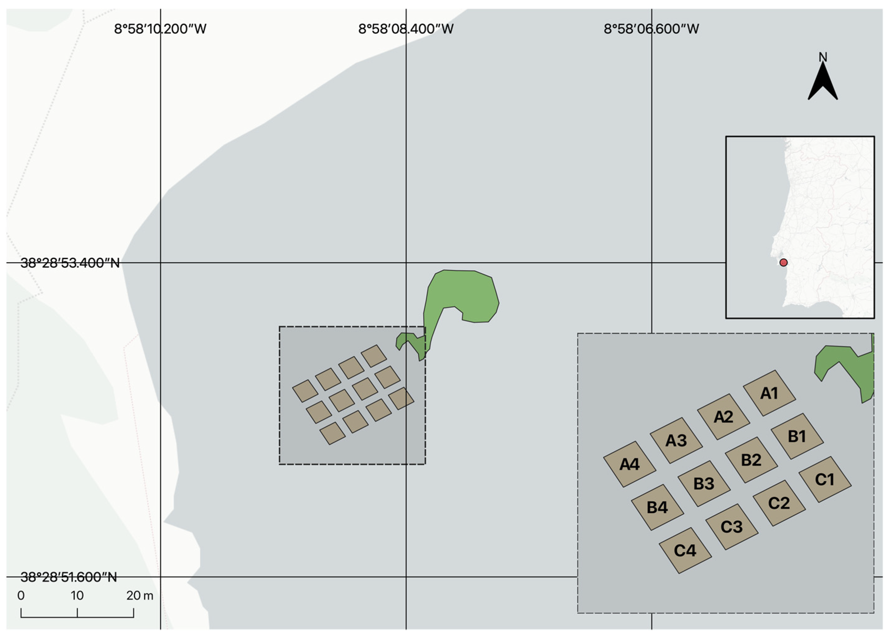
2.1. Site Description

The transplantation efforts were undertaken at the Professor Luiz Saldanha Marine Park, a designated Marine Protected Area (MPA) that is an integral part of the larger Arrábida Natural Park in Portugal. Encompassing an area of 52 km² and spanning a 38 km coastline, the park features an impressive rocky terrain with towering cliffs interspersed with sandy coves. It is within these sandy coves, which are characterized by a sandy substrate, that a seagrass habitat existed previously [30] and successful transplantation endeavours were undertaken in 2010 [14]. Specifically, the transplantation area is situated in Praia dos Coelhos, between the previously restored seagrass meadow (2010) and the rocky cliff that delineates the sandy cove.

2.2. Donor Population

The selection of the donor population for the transplantation operation was conducted with meticulous care, adhering to general guidelines for seagrass restoration [11,12,19,20] and considering the recommendations from the previous study [14]. Various factors, including species composition, seagrass abundance, and overall population health, were thoroughly assessed during the selection process. Among the potential donor populations, the Sado Estuary was identified as the most suitable choice. Located approximately 5–10 km east of the transplant areas, it met all the necessary criteria for Z. marina; however, due to seasonal variations, the Z. noltei populations exhibited low densities. Therefore, the only viable option for Z. noltei was Ria Formosa, a coastal lagoon located 250 km south of the transplant area. While it is extensively covered by seagrass species, including Z. marina and Z. noltei [31], the presence of the invasive species Caulerpa prolifera compromised the suitability of the subtidal populations for transplantation therefore Z. noltei was sourced only from the intertidal population.

2.3. Harvest Method and Transportation

The harvesting technique employed during the project followed the methods described in the 2010 trials [14]. Segments of seagrass sods, including seagrasses and their original sediment, were collected in sections measuring approximately 35 × 35 × 5 cm (sediment depth). Skilled SCUBA divers utilised shovels to carefully extract the sods from the existing meadows. Once collected, the sods were promptly placed in non-buoyant plastic trays measuring 1 m by 0.5 m. To ensure the seagrasses remained in optimal condition, the trays were lifted onto the boat and transported to the designated transplant site (in under 30 min). Throughout the journey, the seagrass was consistently kept wet to prevent drying or any potential damage to the plants. The plants experienced a brief period of air exposure, lasting less than 15–20 min. This brief timeframe was solely required for the relocation process from the harvesting site to the designated transplant site. In addition to the boat, Z. noltei sods also undertook a 3 h car drive from Ria Formosa in a shaded tank.

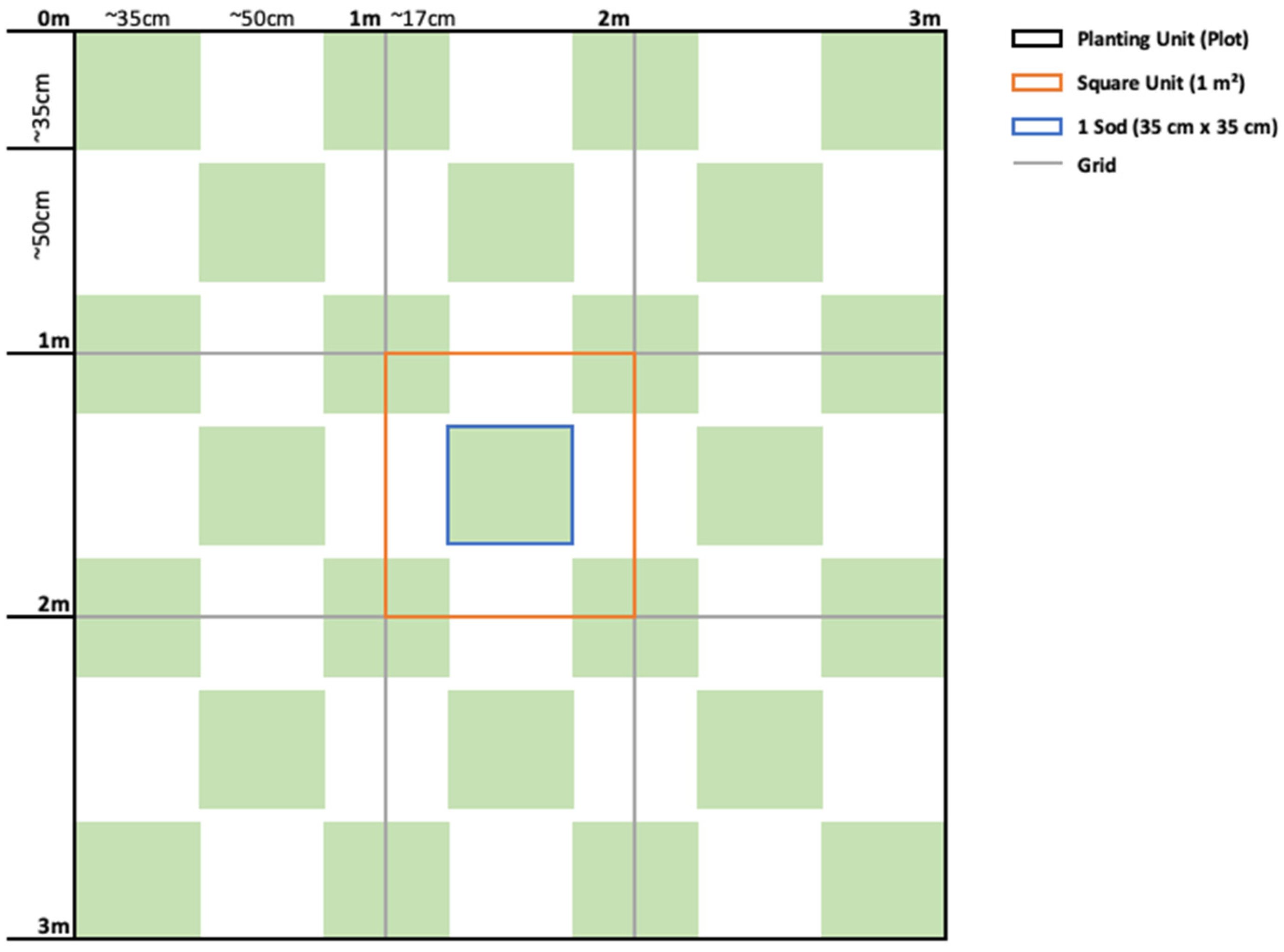
2.4. Transplant Methodology

Within the designated transplant area, a total of twelve 3 × 3 m plots were established for transplantation. These plots were divided into three rows of four, with a one-meter distance separating each (Figure 1). Within each plot, the transplant method involved the placement of 25 seagrass sods measuring 35 × 35 × 5 cm (sediment depth). The sods were arranged in a chessboard pattern, with the corners of each sod positioned near one another (Figure 2). To ensure proper integration with the surrounding seabed, the area where each sod was to be placed was carefully excavated using a shovel until it reached a depth of 5 cm below the surface. This crucial step facilitated the alignment of the sods with the substrate surface. Subsequently, the sods were gently positioned within the excavated holes, and sand was gently pushed to cover the rhizomes, ensuring no roots were left exposed. Once the transplantation process was completed, the entire area was meticulously levelled to achieve a flush surface. Half of the plots were transplanted with Z. marina, and the other half with Z. noltei. The assignment of species to each plot was randomized to ensure unbiased distribution.

2.5. Monitoring and Statistics

The monitoring schedule consisted of multiple monitoring events at specific time intervals. The first monitoring event took place on the day following the transplantation effort, allowing for an initial assessment of the newly transplanted plots. The subsequent monitoring events were conducted approximately one month later and then at intervals of six months.

Due to the size of the transplant operation and logistical considerations, the first monitoring event for each plot occurred at different time points. Specifically, on 1 May 2022, Plots A1, A2, C1, and C2 were transplanted and subsequently monitored. The second monitoring campaign occurred on 25 May, when plots A3, B1, B2, and B3 were transplanted. Lastly, Plots A4, B4, C3, and C4 were transplanted on 24 June and monitored a month after.

During each monitoring event, the plot area was determined by measuring and multiplying the plot sides to obtain the total area in square meters. The assessment of percentage cover was conducted in situ using a 1 m² quadrat divided into 100 squares. All squares within the quadrat where plants were visible were counted. This sampling method was applied to the entire extent of each plot, providing an estimation of the percentage cover of plants within the plot.

To determine shoot density, a systematic sampling approach was implemented. Splitting the 3 × 3 m grid into nine 1 m² areas within each plot, a random selection of 3 m² was chosen for analysis. The entire 3 m² area was sampled using 100 × 100 cm quadrats for Z. marina. For Z. noltei, a smaller quadrat measuring 10 × 10 cm was employed; as such, within each of the randomly selected 3 m² areas, three quadrats were sampled, resulting in a total of nine quadrats per plot. This sampling methodology ensured an accurate assessment of shoot density for both seagrass species in the respective plots, considering that empty spaces were expected between sods and counting Z. noltei shoots in a full square meter would be impractical due to the time requirements while SCUBA diving.

In addition, leaf length (in centimetres) was measured in all plots. The length of each shoot was measured from the sediment to the end of the longest leaf within the quadrats used for density sampling. A minimum of 10 shoots within the quadrats were recorded, resulting in a total of at least 30 shoot length measurements per plot.

To assess the progress of the transplants, we examined changes in absolute area, percent cover, vegetated area (calculated as total area multiplied by percent cover), shoot density, and leaf length across monitoring events for each plot. The plots were then grouped by species to analyze species-specific trends and compare the effectiveness of the methodology between them. All statistical analysis and generation of graphical output were conducted using R Studio (version 2023.3.0.386) [32]. Comparisons of density and leaf length were performed with Linear Mixed-effects Models (LMM), using the “lme” function from the “nlme” package (version 3.1-162) [33,34]. Fixed factors encompassed time, species, and their interactions, while plot position served as the random factor [33,34]. Maps were created using QGIS software (version 3.10) [35].

3. Results

Both species exhibited a seasonal cycle of decline and recuperation, yet the peripheral plots within the transplantation region demonstrated limited or non-existent recovery after one year. This phenomenon was consistent for both species. During monitoring events, some sods were observed to be slightly buried by sand ripples. Consequently, we deduce that the spatial positioning of the plots played a pivotal role in their survival, likely attributable to hydrodynamic factors and direct vulnerability to storms originating from the south (Figure 3). Such storms are part of the factors that can disturb seagrass meadows behind the stable state threshold leading the area to bare sediment, as observed in a natural seagrass meadow nearby [36].

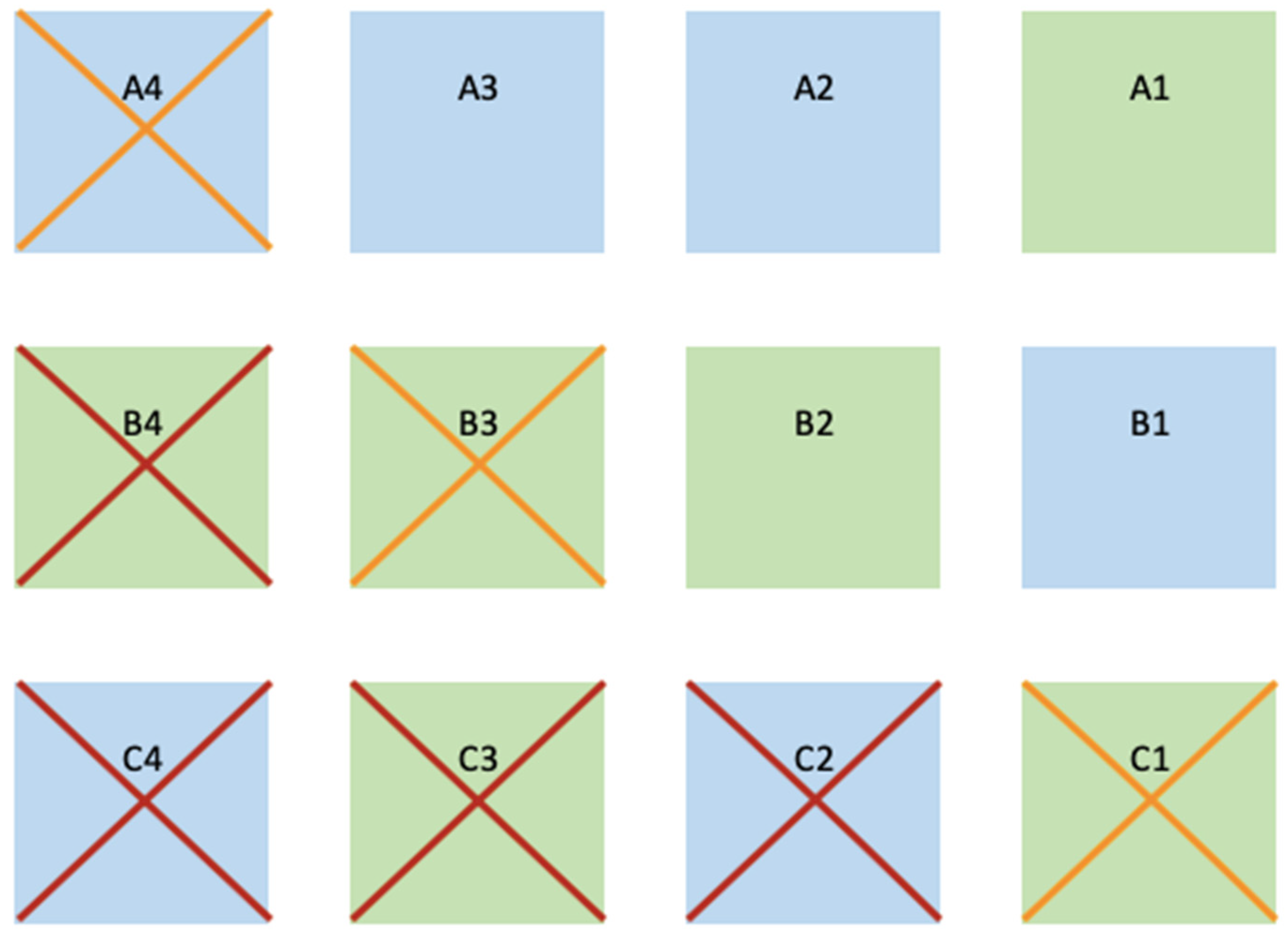
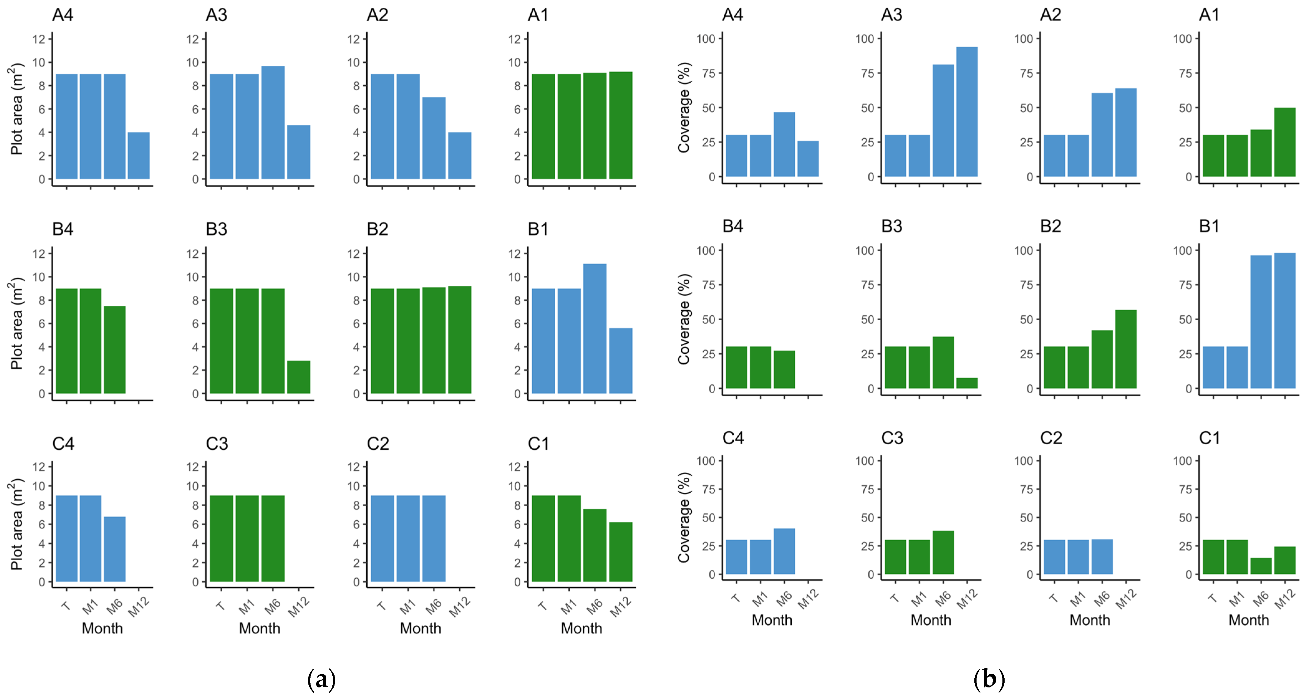
3.1. Plot Survival and Outcome

3.1.1. Z. marina

At the end of the trial, plots A2, A3, and B1 persisted (inner plots) while plots C2 and C4 disappeared and plot A4 was in poor condition (outer plots).

Upon examining the inner plots, until the M6 monitoring event (end of Autumn), plots A3 and B1 increased in absolute area to 9.7 m² and 11.1 m², while plot A2 decreased to 7 m² (Figure 4a). When considering only the vegetated area, at M6, all plots increased from 3.06 m² to 4.23 m² (plot A2), 7.86 m² (plot A3), and 10.68 m² (plot B1). Nevertheless, it is worth noting that the absolute plot areas suffered a substantial reduction during the winter period, with plot A2 shrinking from 9 m² to 4 m², plot A3 decreasing to 4.6 m², and plot B1 diminishing to 5.6 m² (Figure 4a). Accompanying the loss in absolute area there were losses in vegetated area. Despite these losses, and when comparing to the transplant event, the surviving plots A3 and B1 increased from 3.06 m² to 4.31 m² and 5.5 m², respectively, and plot A2 decreased to 2.56 m². From transplant to M12 (Spring 2023), there was an increase in percent cover (Figure 4b). Specifically, the percent cover increased from 35.39% to 64% in plot A2, 93.75% in plot A3, and 98.22% in plot B1. Shoot density increased in the three plots by M6 and decreased to M12. Still, from transplant to M12, plot B1 (p = 0.00) increased density from 99.33 ± 14.52 shoots·m⁻² to 313.33 ± 61.33 shoots·m⁻². In plots A2 and A3, the differences in shoot density were not significant after one year (p > 0.05), although there was a slight increase (Figure 5). Regarding leaf length, all plots decreased (p < 0.01) (Figure 6). These results provide evidence for the dynamic changes occurring within the plots, with variations in percent cover, shoot density, and leaf length over the course of one year.

Examining the outer plots, plots C2 and C4 disappeared after the winter season. Plot A4 exhibited a decrease in all measured parameters (area, percent cover, density, and leaf length), decreasing to an area of 4 m² with a percent cover of 25.8% and a density of 15.67 ± 1.20 shoots·m⁻² at the M12 event (Figure 4, Figure 5 and Figure 6). Concerning vegetated area, it decreased from 3.06 m² to 1.03 m². Density and leaf length also decreased from transplant to M12 (p < 0.05).

Notably, until the M6 event, density increased in plots A4 (p = 0.04) and C2 (p < 0.01) and decreased in plot C4 (p < 0.01), which is a similar pattern to the inner plots (Figure 5). However, the absolute area was constant at 9 m² in plots A4 and C2, decreasing to 6.8 m² in C4; with only a slight increase in percent cover (46.72%, 30.78%, and 40.33%, respectively) (Figure 4). Furthermore, the vegetated area only grew in plot A4 to 4.2 m² with the other two very close to the original vegetated area. These findings suggest that the outer plots were likely subject to stronger environmental conditions and were unable to adapt as effectively as the inner plots. The reduced percent cover and lower density in plot A4 after winter indicate the challenges faced by the outer plots in sustaining vegetation and highlight their lesser ability to cope with the prevailing environmental conditions.

3.1.2. Z. noltei

The inner plots of Z. noltei consist of plots A1, B2, and B3. Plot B3, albeit not technically located in the periphery, was also impacted, and found to be mostly buried in sand. Likewise, the outer plots B4 and C3 disappeared completely, while plot C1 displayed a gradual regression.

In the inner plots A1 and B2 there was an increase in area and percent cover over time (Figure 4), achieving 9.1 m² by M6 and with a slight increase in percent cover, converting to a slight increase in vegetated area to 3.1 m² (A1) and 3.83 m² (B2). By the end of the trial, both plots had expanded from 9 m² to 9.2 m², with plot A1 presenting a coverage of 49.89% and plot B2 a coverage of 56.78%. This translates to 4.59 m² and 5.22 m² of vegetated area, respectively. Both plots had an increase in shoot density, from 1441.92 ± 86.15 shoots·m⁻² to 2145.27 ± 137.64 shoots·m⁻² in plot A1 (p < 0.01), and from 1441.92 ± 139.35 shoots·m⁻² to 1854.81 ± 73.30 shoots·m⁻² in plot B2 (p = 0.02) (Figure 5). Mean leaf length was lower compared to the initial measurements in both plots (p < 0.01) (Figure 6). Overall, the inner plots experienced an increase in size, coverage, and shoot density. However, there was a noticeable decrease in leaf length for both plots after one year of transplant.

Among the outer plots, plots B4 and C3 disappeared during the winter. Plot B3 and C1 persisted, but with less vegetated area than at the transplant event. Plot B3 was observed to be nearly buried during the one-year monitoring event. It exhibited a reduced area of 2.8 m² and coverage of 7.5%, i.e., 0.21 m² of vegetated area (Figure 4). Shoot density (26.25 ± 1.31 shoots·m⁻²) and leaf length (8.43 ± 0.52 cm) also decreased (p < 0.01) (Figure 5 and Figure 6). Like B3, plot C1 experienced a decrease in all measured parameters, being reduced to 6.2 m², a coverage of 24.33% (1.51 m² of vegetated area), a decrease in shoot density (656.91 ± 9.93 shoots·m⁻²), and leaf length (9.63 ± 0.63 cm) (p < 0.01). These observations indicate that plot B3 suffered from burial by sediment, resulting in a lower coverage and shoot density. In contrast with B4 and C3, plot C1 resisted and showed a slight recovery from M6 to M12, but also experienced a decrease in all parameters.

3.2. Species Comparison on Methodology Success

The three inner plots of Z. marina were grouped together, resulting in a transplanted absolute area of 27 m² with a cover of 30.35% (9.19 m² of vegetated area). The average shoot density was 80 ± 13.57 shoots·m⁻², and the leaves measured 26.38 ± 0.65 cm. In the first six months (M6) the area increased to 27.8 m² and 81.87% cover, meaning 22.77 m² of vegetated area (an increase of 147.73%) (Figure 4). Density increased to 330.78 ± 60.38 shoots·m⁻² (313.47%) (p < 0.01) (Figure 5) and leaf length decreased to 17.22 ± 0.47 cm (34.75%) (p < 0.01) (Figure 6). From transplant to M12, the absolute area decreased to 14.2 m², but the percent cover increased to 87%, meaning the vegetated area increased by 34.5% to 12.36 m² (Figure 4). Density showed a tendency to increase, with 164.6 ± 39.41 shoots·m⁻² (p > 0.05) (Figure 5), while leaf length decreased to 21.29 ± 0.52 cm (p < 0.01) (Figure 6). In other words, over winter occurred a decrease in vegetated area (45.7%) and density (50.21%) (p < 0.05), but an increase in leaf length (23.65%) (p < 0.01).

Grouping the two inner plots of Z. noltei, we observed a steady increase in various parameters over a year. At transplant, we had an area of 18 m² and 30.35% coverage (6.13 m² of vegetated area), a density of 1441.92 ± 79.47 shoots·m⁻², and a leaf length of 14.14 ± 0.39 cm. At the M6 event, the absolute area went to 18.2 m² and 38.05% coverage (6.93 m² of vegetated area) (Figure 4). Density increased (1566.16 ± 118.56 shoots·m⁻²) (p < 0.01) (Figure 5) and leaf length decreased (9.81 ± 0.59 cm) (p < 0.01) (Figure 6). From transplant to M12 there was an increase in absolute area (to 18.4 m²), percentage cover (53.31%), vegetated area (9.81 m²), and density (2000.04 ± 83.44 shoots·m⁻²) (p < 0.01), accompanied by a decrease in leaf length (8.91 ± 0.37 cm) (p < 0.01) (Figure 4, Figure 5 and Figure 6). From M6 to M12, there was a slight increase in area (1.10%) but was more pronounced in percent cover (40.11%) and vegetated area (41.60%). Density also increased (27.70%) while leaf length decreased (9.81%).

Both species exhibited an increase in percent cover and density, which varied over time between species (Figure 4 and Figure 5). But while there were small changes in the relative density difference between the species from month to month, the impact of each month on the overall density is small. Leaf length was influenced by month, with negative coefficients indicating a decrease as time progressed, a more pronounced decrease by M6 and a slight recovery by M12 (Figure 4, Figure 5 and Figure 6). The relationship between leaf length and the passage of time differed across species with Z. noltei exhibiting greater variations. Overall, Z. marina exhibited the highest increase during the first 6 months, lost area during winter but still showed a substantial increase in percent cover (187.4%), shoot density (105.8%) and vegetated area (34.5%) a year after transplant. In contrast, Z. noltei demonstrated a more modest increase in the first six months, which seemed to continue over winter—all parameters but leaf length increased. A year after transplant Z. noltei showed a smaller but considerable increase in percent cover (76.1%) and density (38.7%) but greater vegetated area (60.22%) than Z. marina. It should be noted that this success was not consistently observed in plots located on the south periphery of the grid-like transplant design (Figure 3).

4. Discussion

This study provides evidence of the efficacy of the checkers methodology, which uses less vegetation per area at the transplant event, in comparison to the mega plot method described by Paulo et al. [14] that transplanted areas of 100% cover larger than 6 m². Checkers is therefore 66.68% more efficient in plant usage than the mega plot.

The growth outcomes in our method look more promising than in a planting units (PUs) method that used corers of 24 cm diameter to harvest sods, as described in Curiel et al. [16] with Z. marina. In our study, sods were observed to coalesce two months earlier (month 6) than in Curiel et al., and there was higher survival of sods (called PUs). Unfortunately, we cannot compare the end of both studies as the reported data is for month 17 (September) and our data ends in month 12 (May). This would imply that the comparison made with our study would not consider the periods of peak growth reported for the species [37]. Nevertheless, the results look promising as we observed increased percentage coverage, density, and vegetated area for both Z. marina and Z. noltei after one year.

Despite the positive fitness indicators for both species, differences between species were observed. Z. noltei demonstrated a slower sod expansion but an increase in absolute area as it resisted loss during winter storms. In comparison, Z. marina grew faster, exhibiting a more substantial increase in density and cover, despite losing some area during winter.

Survivability seemed to not be related to the methodology or be species specific. Plot disappearance was most prevalent in the south-facing plots, where the coast is exposed. As the area is defined by strong tidal currents and prevalent south winter storms [30], it suggests survival was location dependent. In 2017 [14], transplant trials were lost over winter and as the sampling design was smaller (six plots), this spatial trend of outer seaward marginal biomass loss was not apparent. Our study has doubled their plot numbers (12 plots), facilitating a spatial analysis contrasting survival between plots closer or more distal from the coastline. In the previous study, the loss of these plots coincided with the Sado estuary population as a donor. However, in this study, we have used that donor population with success, suggesting the loss was location-dependent and not caused by using a specific species or donor population.

In comparing the success of each species over the course of a year, both showed good survival and growth, but at different degrees. The sods of Z. marina expanded rapidly in the first semester, in some plots close to or more than tripling its vegetated area. By analyzing each individual parameter, we can conclude each sod expanded and coalesced, creating a dense meadow with high cover, and attaining the basic concept of the checkers method. Each sod comprised several ramets that will expand into unvegetated areas, and as the number of ramets increases, so does its cumulative growth, in turn increasing its expansion rate [38]. Even so, these results were still surprising for such a short time span (6 months), demonstrating that Z. marina can be a fast colonizer once transplanted. Despite this, the winter season had a big impact on the surviving plots, and of them, all lost areas during this season. This outcome was expected, since during winter seasons the limitation of light and harsh hydrodynamics caused by storms affect seagrasses [2,39]. But, contrary to our expectations that Z. noltei plots would be the species where plants would merge faster [38,40], Z. noltei plots demonstrated a slower and steadier growth, and, contrary to Z. marina, a notable resistance to the winter season as there was no loss of area or density. This resistance may be explained by the flexibility of its leaves which can stay horizontal at high current speeds, reducing canopy drag [41]. It is important to note that the resilience in Z. marina plots appears to have been achieved as density and leaf length were comparable with established meadows. Still, our focus was on testing a new methodology and the data collected mirrors that objective. Reflecting on the unexpected expansion rates observed in this study, we suggest a new study focusing on the adaptability of the species after a transplant event.

Our results indicate that the most critical factor to consider at the site is the presence of strong currents and storms. We note that not all replicates could be used to assess the success of the methodology, but the available data shows promising results in the surviving plots. This confirms the site is undoubtedly suitable for seagrass and that the transplantation methodology is effective. Still, to minimize the loss of transplants, measures must be taken to enhance their protection, or enough biomass should be planted simultaneously to counteract the destructive power of storms.

Based on the comprehensive results and inherent limitations, this study provides a significant indication of the success of the new checkers methodology. It also raises three interconnected questions that require attention for a large-scale restoration effort: (1) the placement of sods, (2) the selection of donor populations, and (3) the associated costs. These questions are critical for further research and implementation of the methodology.

Successful seagrass restoration requires considering a combination of individual factors [10]. While previous research has focused on broader-scale assessments, this study highlights the spatial heterogeneity within small areas, emphasizing the need for a comprehensive understanding of the site. To maximize restoration success at a local scale, it is crucial to strategically select transplant sites that offer the highest ecological benefits and potential for long-term survival. This may involve transplanting in favorable locations and implementing measures to mitigate potential impacts until the desired ecological state is achieved.

By selecting and preparing the most suitable site, we also maximize donor biomass, particularly for large-scale efforts. While small-scale trials often utilise local meadows with no apparent impact [16,22,26,28], sourcing sufficient biomass for large-scale trials becomes challenging and may be unadvised [31]. Relying solely on plant collection from natural populations is intrusive, risks ecological impacts and, as previously stated, restoration through seeds takes commitment and needs time [22,23,24,25]. One possible solution to source plants other than from existing meadows could be the growth of biomass in aquaculture facilities. These facilities offer controlled environments for optimal seagrass cultivation, enabling extensive and efficient transplantation.

Despite this, the success of restoration projects is heavily influenced by funding availability. Although the potential for habitat and biodiversity improvement exists, financial constraints pose significant challenges [42]. Limited funding can restrict the scale, frequency, and extent of seagrass transplantation, as well as monitoring events and maintenance efforts [43]. In this study, with a team of three technicians, the transplants were done in four work-intensive campaigns of three days each (material collection, travel, and transplant). Considering the actual average costs in Portugal (technician salary, boat fuel, and van expenses), the transplant cost an estimated EUR 25 per m².

While knowledge of large-scale restoration is growing, large-scale trials are still limited [19]. Collaboration between government agencies, research institutions, non-profit organisations, and the private sector can help pool resources and expertise. Increasing awareness about the ecological value of seagrass ecosystems and their services can also attract diverse funding sources [43]. Strategic planning and prioritization are crucial for optimising limited funds. By addressing these issues, large-scale habitat restoration is feasible, and our methodology maximizes the use of available biomass to expand restoration areas and transform unvegetated systems into vegetated systems, providing all the ecosystem services seagrasses can offer.

References

1. Cullen-Unsworth, L.C.; Unsworth, R.K.F. Strategies to Enhance the Resilience of the World’s Seagrass Meadows. J. Appl. Ecol. 2016, 53, 967–972. [Google Scholar] [CrossRef]
2. Green, E.P.; Short, F.T. World Atlas of Seagrasses, 1st ed.; University of California Press: Berkeley, CA, USA, 2003; p. 21. [Google Scholar]
3. Cullen-Unsworth, L.C.; Nordlund, L.M.; Paddock, J.; Baker, S.; McKenzie, L.J.; Unsworth, R.K.F. Seagrass Meadows Globally as a Coupled Social-Ecological System: Implications for Human Wellbeing. Mar. Pollut. Bull. 2014, 83, 387–397. [Google Scholar] [CrossRef] [PubMed]
4. Nordlund, L.M.; Koch, E.W.; Barbier, E.B.; Creed, J.C. Seagrass Ecosystem Services and Their Variability across Genera and Geographical Regions. PLoS ONE 2016, 11, e0163091. [Google Scholar] [CrossRef]
5. Duarte, C.M.; Losada, I.J.; Hendriks, I.E.; Mazarrasa, I.; Marbà, N. The Role of Coastal Plant Communities for Climate Change Mitigation and Adaptation. Nat. Clim. Chang. 2013, 3, 961–968. [Google Scholar] [CrossRef]
6. Fourqurean, J.W.; Duarte, C.M.; Kennedy, H.; Marbà, N.; Holmer, M.; Mateo, M.A.; Apostolaki, E.T.; Kendrick, G.A.; Krause-Jensen, D.; McGlathery, K.J.; et al. Seagrass Ecosystems as a Globally Significant Carbon Stock. Nat. Geosci. 2012, 5, 505–509. [Google Scholar] [CrossRef]
7. Short, F.T.; Polidoro, B.; Livingstone, S.R.; Carpenter, K.E.; Bandeira, S.; Bujang, J.S.; Calumpong, H.P.; Carruthers, T.J.B.; Coles, R.G.; Dennison, W.C.; et al. Extinction Risk Assessment of the World’s Seagrass Species. Biol. Conserv. 2011, 144, 1961–1971. [Google Scholar] [CrossRef]
8. Waycott, M.; Duarte, C.M.; Carruthers, T.J.B.; Orth, R.J.; Dennison, W.C.; Olyarnik, S.; Calladine, A.; Fourqurean, J.W.; Heck, K.L.; Hughes, A.R.; et al. Accelerating Loss of Seagrasses across the Globe Threatens Coastal Ecosystems. Proc. Natl. Acad. Sci. USA 2009, 106, 12377–12381. [Google Scholar] [CrossRef]
9. Curiel, D.; Pavelić, S.K.; Kovačev, A.; Miotti, C.; Rismondo, A. Marine Seagrasses Transplantation in Confined and Coastal Adriatic Environments: Methods and Results. Water 2021, 13, 2289. [Google Scholar] [CrossRef]
10. Tan, Y.M.; Dalby, O.; Kendrick, G.A.; Statton, J.; Sinclair, E.A.; Fraser, M.W.; Macreadie, P.I.; Gillies, C.L.; Coleman, R.A.; Waycott, M.; et al. Seagrass Restoration Is Possible: Insights and Lessons from Australia and New Zealand. Front. Mar. Sci. 2020, 7, 617. [Google Scholar] [CrossRef]
11. Calumpong, H.P.; Fonseca, M.S. Seagrass transplantation and other seagrass restoration methods. In Global Seagrass Research Methods, 1st ed.; Short, F.T., Coles, R.G., Eds.; Elsevier Science B.V.: Amsterdam, The Netherlands, 2001; Volume 1, pp. 425–443. [Google Scholar]
12. Paling, E.I.; Fonseca, M.; van Katwijk, M.M.; van Keulen, M. Seagrass Restoration. In Coastal Wetlands: An Integrated Ecosystem Approach, 1st ed.; Perillo, G., Wolanski, E., Cahoon, D., Brinson, M., Eds.; Elsevier Science: Amsterdam, The Netherlands, 2009; pp. 687–713. ISBN 978-008-093-213-2. [Google Scholar]
13. Paling, E.I.; van Keulen, M.; Wheeler, K.D.; Phillips, J.; Dyhrberg, R. Influence of Spacing on Mechanically Transplanted Seagrass Survival in a High Wave Energy Regime. Restor. Ecol. 2003, 11, 56–61. [Google Scholar] [CrossRef]
14. Paulo, D.; Cunha, A.H.; Boavida, J.; Serrão, E.A.; Gonçalves, E.J.; Fonseca, M. Open Coast Seagrass Restoration. Can We Do It? Large Scale Seagrass Transplants. Front. Mar. Sci. 2019, 6, 52. [Google Scholar] [CrossRef]
15. Wegoro, J.; Pamba, S.; George, R.; Shaghude, Y.; Hollander, J.; Lugendo, B. Seagrass Restoration in a High-Energy Environment in the Western Indian Ocean. Estuar. Coast. Shelf Sci. 2022, 278, 108119. [Google Scholar] [CrossRef]
16. Curiel, D.; Scarton, F.; Rismondo, A.; Marzocchi, M. Pilot transplanting project of Cymodocea nodosa and Zostera marina in the lagoon of Venice: Results and perspectives. Boll. Mus. Civ. St. Nat. Venezia 2005, 56, 25–40. [Google Scholar]
17. Turner, S.J.; Hewitt, J.E.; Wilkinson, M.R.; Morrisey, D.J.; Thrush, S.F.; Cummings, V.J.; Funnell, G. Seagrass Patches and Landscapes: The Influence of Wind-Wave Dynamics and Hierarchical Arrangements of Spatial Structure on Macrofaunal Seagrass Communities. Estuaries 1999, 22, 1016–1032. [Google Scholar] [CrossRef]
18. Fonseca, M.S.; Bell, S.S. Influence of Physical Setting on Seagrass Landscapes. Mar. Ecol. Prog. Ser. 1998, 171, 109–121. [Google Scholar] [CrossRef]
19. Katwijk, M.M.; Thorhaug, A.; Marbà, N.; Orth, R.J.; Duarte, C.M.; Kendrick, G.A.; Althuizen, I.H.J.; Balestri, E.; Bernard, G.; Cambridge, M.L.; et al. Global Analysis of Seagrass Restoration: The Importance of Large-scale Planting. J. Appl. Ecol. 2016, 53, 567–578. [Google Scholar] [CrossRef]
20. Campbell, M.L. Getting the Foundation Right: A Scientifically Based Management Framework to Aid in the Planning and Implementation of Seagrass Transplant Efforts. Bull. Mar. Sci. 2002, 71, 1405–1414. [Google Scholar]
21. Holling, C.S. Resilience and Stability of Ecological Systems. Annu. Rev. Ecol. Syst. 1973, 4, 1–23. [Google Scholar] [CrossRef]
22. Govers, L.L.; Heusinkveld, J.H.T.; Gräfnings, M.L.E.; Smeele, Q.; van der Heide, T. Adaptive Intertidal Seed-Based Seagrass Restoration in the Dutch Wadden Sea. PLoS ONE 2022, 17, e0262845. [Google Scholar] [CrossRef]
23. Marion, S.R.; Orth, R.J. Factors Influencing Seedling Establishment Rates in Zostera Marina and Their Implications for Seagrass Restoration. Restor. Ecol. 2010, 18, 549–559. [Google Scholar] [CrossRef]
24. Orth, R.; McGlathery, K.; Cole, L. Eelgrass Recovery Induces State Changes in a Coastal Bay System. Mar. Ecol. Prog. Ser. 2012, 448, 173–176. [Google Scholar] [CrossRef]
25. Sinclair, E.A.; Sherman, C.D.H.; Statton, J.; Copeland, C.; Matthews, A.; Waycott, M.; van Dijk, K.J.; Vergés, A.; Kajlich, L.; McLeod, I.M.; et al. Advances in Approaches to Seagrass Restoration in Australia. Ecol. Manag. Restor. 2021, 22, 10–21. [Google Scholar] [CrossRef]
26. Matheson, F.E.; Reed, J.; Dos Santos, V.M.; Mackay, G.; Cummings, V.J. Seagrass Rehabilitation: Successful Transplants and Evaluation of Methods at Different Spatial Scales. N. Z. J. Mar. Freshwater. Res. 2017, 51, 96–109. [Google Scholar] [CrossRef]
27. Mokumo, M.F.; Adams, J.B.; von der Heyden, S. Investigating Transplantation as a Mechanism for Seagrass Restoration in South Africa. Restor. Ecol. 2023. [Google Scholar] [CrossRef]
28. Ranwell, D.S.; Wyer, D.W.; Boorman, L.A.; Pizzey, J.M.; Waters, R.J. Zostera Transplants in Norfolk and Suffolk, Great Britain. Aquaculture 1974, 4, 185–198. [Google Scholar] [CrossRef]
29. Fonseca, M.S. A Guide to Planting Sea Grasses in the Gulf of Mexico, 1st ed.; Sea Grant College Program, Texas A&M University: College Station, TX, USA, 1993; pp. 1–25. [Google Scholar]
30. Cunha, A.H.; Assis, J.F.; Serrão, E.A. Seagrasses in Portugal: A Most Endangered Marine Habitat. Aquat. Bot. 2013, 104, 193–203. [Google Scholar] [CrossRef]
31. Cunha, A.H.; Assis, J.; Serrão, E.A. Estimation of Available Seagrass Meadow Area in Portugal for Transplanting Purposes. J. Coast. Res. 2009, 56, 1100–1104. [Google Scholar]
32. R Core Team. 2023. R: A Language and Environment for Statistical Computing (2023.3.0.386). MacOS. Austria: R Foundation for Statistical Computing. Available online: https://www.R-project.org/ (accessed on 28 June 2023).
33. Pinheiro, J.C.; Bates, D.M.; R Core Team. Nlme: Linear and Nonlinear Mixed Effects Models (3.1-162); MacOS: New York, NY, USA, 2003. [Google Scholar]
34. Pinheiro, J.C.; Bates, D.M. Mixed-Effects Models in S and S-PLUS, 1st ed.; Statistics and Computing; Springer-Verlag: New York, NY, USA, 2000; pp. 1–113. [Google Scholar]
35. QGIS Department Team. QGIS Geographic Information System (3.10). 2020. Available online: https://qgis.org/en/site/ (accessed on 20 May 2023).
36. Paulo, D.; Diekmann, O.; Ramos, A.A.; Alberto, F.; Serrão, E.A. Sexual Reproduction vs. Clonal Propagation in the Recovery of a Seagrass Meadow after an Extreme Weather Event. Sci. Mar. 2019, 83, 357–363. [Google Scholar] [CrossRef]
37. Zimmerman, R.C.; Reguzzoni, J.L.; Alberte, R.S. Eelgrass (Zostera marina L.) Transplants in San Francisco Bay: Role of Light Availability on Metabolism, Growth and Survival. Aquat. Bot. 1995, 51, 67–86. [Google Scholar] [CrossRef]
38. Borum, J. European Seagrasses: An Introduction to Monitoring and Management; Monitoring and Managing of European Seagrasses [EU Project]; The M&MS Project: Copenhagen, Denmark, 2004; ISBN 8789143213. [Google Scholar]
39. Van Der Heide, T.; Van Nes, E.H.; Geerling, G.W.; Smolders, A.J.P.; Bouma, T.J.; Van Katwijk, M.M. Positive Feedbacks in Seagrass Ecosystems: Implications for Success in Conservatiooutln and Restoration. Ecosystems 2007, 10, 1311–1322. [Google Scholar] [CrossRef]
40. Cunha, A.H.; Santos, R.P.; Gaspar, A.P.; Bairros, M.F. Seagrass Landscape-Scale Changes in Response to Disturbance Created by the Dynamics of Barrier-Islands: A Case Study from Ria Formosa (Southern Portugal). Estuar. Coast. Shelf. Sci. 2005, 64, 636–644. [Google Scholar] [CrossRef]
41. Widdows, J.; Pope, N.D.; Brinsley, M.D.; Asmus, H.; Asmus, R.M. Effects of Seagrass Beds (Zostera noltii and Z. marina) on near-Bed Hydrodynamics and Sediment Resuspension. Mar. Ecol. Prog. Ser. 2008, 358, 125–136. [Google Scholar] [CrossRef]
42. Bayraktarov, E.; Saunders, M.I.; Abdullah, S.; Mills, M.; Beher, J.; Possingham, H.P.; Mumby, P.J.; Lovelock, C.E. The Cost and Feasibility of Marine Coastal Restoration. Ecol. Appl. 2015, 26, 1055–1074. [Google Scholar] [CrossRef] [PubMed]
43. Danovaro, R.; Aronson, J.; Cimino, R.; Gambi, C.; Snelgrove, P.V.R.; Van Dover, C. Marine Ecosystem Restoration in a Changing Ocean. Restor Ecol 2021, 29, e13432. [Google Scholar] [CrossRef]
Figure 1. Map of the transplant area in Praia dos Coelhos, Arrábida, Portugal. In green, the established meadow transplanted in 2010. In brown, the 12 plots (9 m2 each) displayed in a grid pattern and separated by a meter between themselves. From north to south, the rows are defined as “A”, “B”, and “C”. From east to west plots are numbered 1 to 4.
Sustainability 15 12937 g001
Figure 2. Representation of the checkers methodology. A grid was mounted at every meter (grey lines), creating nine square units (orange outline) within each planting unit of 3 × 3 m (black outline). The sods (in green) were transplanted in a checkerboard pattern, separated by approximately 50 cm and with the corners in proximity.
Sustainability 15 12937 g002
Figure 3. Representation of the outcome of the plots considering its spatial design. In blue background are the plots of Z. marina and in green background of Z. noltei. The red crosses represent the plots that disappeared over winter and in orange the plots left in poor conditions (<2 m2 of vegetated area and low densities). From top to bottom, the rows are defined as “A”, “B”, and “C”. From right to left plots are numbered 1 to 4.
Sustainability 15 12937 g003
Figure 4. Barplot depicting the position of the plots in the field, representing the observed values of (a) plot area (m2) by plot and monitor event; (b) respective percentage cover by plot and monitor event. Green—Z. noltei (plots A1, B2, B3, B4, C1, and C3); blue—Z. marina (plots A2, A3, A4, B2, C2, and C4). T—transplant date; M1—1 month after transplant; M6—6 months after transplant; M12—12 months after transplant.
Sustainability 15 12937 g004
Figure 5. Boxplot on the distribution of density (shoots·m–2) per plot and monitor event. The position of the plots is as in the field. Species are coded by colour, where in blue is Z. marina (plots A2, A3, A4, B1, C2, and C4) and in green is Z. noltei (plots A1, B2, B3, B4, C1, and C3). On the x axis are the monitoring events where T—transplant date, M1—month 1, M6—month 6, and M12—month 12.
Sustainability 15 12937 g005
Figure 6. Boxplot on the distribution of leaf lengths (cm) per plot and monitor event. The position of the plots is as in the field. Species are coded by colour, where in blue is Z. marina (plots A2, A3, A4, B1, C2, and C4) and in green is Z. noltei (plots A1, B2, B3, B4, C1, and C3). On the x axis are the monitoring events where T—transplant date, M1—month 1, M6—month 6, and M12—month 12.
Sustainability 15 12937 g006
Disclaimer/Publisher’s Note: The statements, opinions and data contained in all publications are solely those of the individual author(s) and contributor(s) and not of MDPI and/or the editor(s). MDPI and/or the editor(s) disclaim responsibility for any injury to people or property resulting from any ideas, methods, instructions or products referred to in the content.