Structural Equation Modeling of the Marine Ecological System in Nanwan Bay Using SPSS Amos

Abstract

To ensure the sustainability of the marine environment, it is crucial to understand the intricate relationship between environmental factors and marine biota. Human activities have been recognized as significant contributors to profound changes in marine ecology. However, these observable alterations often represent a cumulative effect that intertwines with less apparent natural influences. This research delved into the relationships between environmental factors and marine life in the waters adjacent to Nanwan Bay, Kenting, Taiwan. Specifically, it examined the linear relationships and the degree of changes between environmental factors and marine life. To achieve these objectives, factor analysis was employed to uncover potential latent variables that could impact marine organisms, with these variables named based on previous studies and related literature. The findings led to the development of a structural equation model (SEM) to represent the marine ecology of Nanwan Bay. The results accentuated the significant influence of primary productivity and nutrient levels on the assemblage of marine life. The application of SEM methodology sheds more light on the degree of impact natural and anthropogenic interference have on marine ecosystems.

1. Introduction

In marine ecosystems, changes in the water temperature reflect the heat balance of seawater and its temporal variation and are also important factors affecting the survival of marine organisms [1]. To support national economic development and industrial growth, many countries, including the United States, China, and Japan, have chosen to build nuclear power plants in coastal areas to supply electricity for daily life and industry. The large amount of heated water discharged from nuclear power plants elevates the sea water temperature, potentially affecting marine organisms. However, the extent of this impact on the local region can also be influenced by site characteristics and environmental background [1]. Previous studies have shown that environmental factors can affect the abundance of marine organisms [2,3]. For instance, the water temperature, light, and nutrient concentration often affect the aggregation structure of phytoplankton, the primary producer in marine ecosystems, in specific times and spaces [4]. Hence, the increase in water temperature caused by discharged heated water may affect the photosynthetic efficiency and species composition of phytoplankton, and may also affect the metabolism of zooplankton, reducing their abundance [5,6,7]. Moreover, changes in prey species and water temperature may cause differences in the distribution of fish [8].

This study was conducted in the semi-enclosed Nanwan Bay, Taiwan, where about ten million tons of cooling seawater have been drawn and discharged every day since May 1984 for the operation of a nuclear power plant. Notably, Kenting National Park was established in 1982, shortly after construction began on the power plant in 1981. The operation of the nuclear plant has since raised significant environmental concerns, leading to active research in the area. Long-term water quality monitoring data indicate that the water temperature changes in the Bay are mainly affected by weather, seasonality, and large-scale ocean events, and are not directly related to the discharge of heated water [9,10]. In an attempt to gain a deeper understanding of how these complex natural phenomena can impact marine ecosystems, it is necessary to investigate the unique influence of strongly interrelated factors. Consequently, this research aims to ascertain the extent of influences wielded by these elusive environmental factors, specifically nutrients and upwelling current, on marine life.

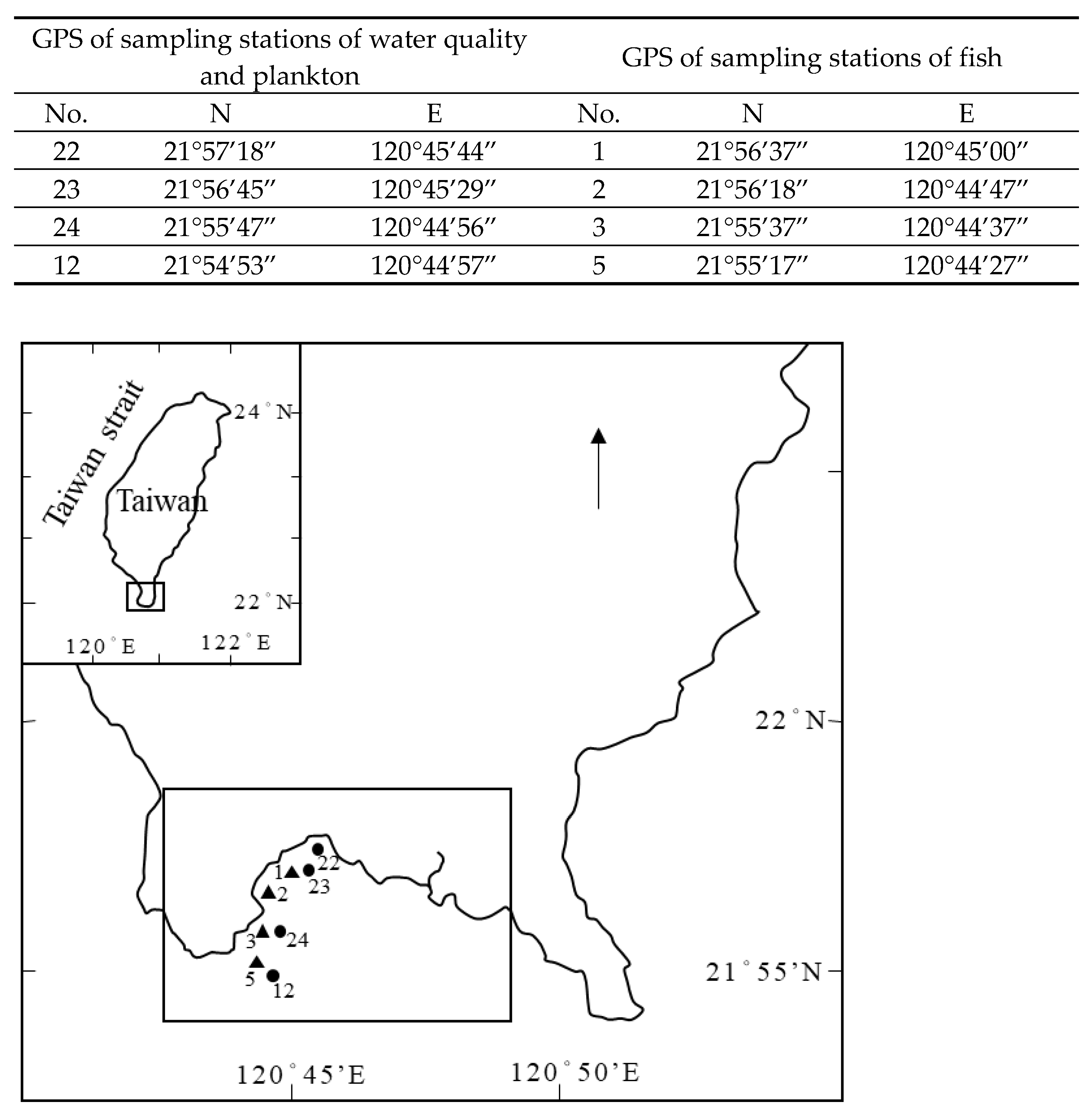
2. Materials and Methods

In this study, we analyzed a total of 223 items of valid water quality and marine biological data surveyed at 4 stations in Nanwan Bay, Kenting, Taiwan, in the same seasons and months, specifically February, May, August, and November from 2000 to 2016 (Figure 1). We employed a multi-stage approach to examine the interrelationships among various factors in the marine environment, with the aim of constructing a structural equation model (SEM), a model which integrates factor analysis and path analysis to analyze data [11,12]. This methodology can not only serve as an approach for theoretical verification, but also incorporates multiple environmental and biological factors into one model. In the first stage, Pearson correlation analysis was used to evaluate the linear association between the variables. Then, factor analysis was conducted to identify common factors among the variables, with these factors subsequently serving as measurement models in SEM.

One issue that can compromise the validity of factor analysis is excessively high or low correlations between variables. To address this, the Kaiser–Meyer–Olkin (KMO) measure, a statistic that compares the magnitude of observed correlation coefficients to the magnitude of partial correlation coefficients, was utilized [13]. In conjunction, Bartlett’s test of sphericity, which checks the overall significance of all the correlations within the correlation matrix, was used. The tests helped to ensure adequate sampling (

Table 1. KMO measurement sampling adequacy criteria (Kaiser, 1974) [12].

KMO Value	Applicability of Factor Analysis
0.9 ≤ KMO	Marvelous
0.8 ≤ KMO ≤ 0.9	Meritorious
0.7 ≤ KMO ≤ 0.8	Middling
0.6 ≤ KMO ≤ 0.7	Mediocre
0.5 ≤ KMO ≤ 0.6	Miserable
KMO ≤ 0.5	Unacceptable

) and sufficient correlation matrices, respectively.

To ensure the validity of the measurement models, we assessed the construct validity. Construct validity encompasses convergent validity, which confirms whether or not measures that should theoretically be related are indeed correlated with corresponding factors, and discriminant validity, which measures how much a construct is distinct from other constructs. We adopted factor loadings of 0.5 and above as a benchmark for convergent validity and specified cross-loadings of below 0.5 to ensure discriminant validity, as suggested by Chen (2005) [14]. Furthermore, we employed communality to quantify the extent to which a variable contributes to a latent factor. The value ranges from 0 to 1, with higher values indicating that the variable is more closely related to the common factor and has lower uniqueness. Thus, variables with high communality are deemed to be more appropriate measurement variables. Consequently, variables with a communality score exceeding 0.5 can be identified as ideal measurement variables, following Chen’s (2005) [14] guideline. After validating these measurements, environment-related literature and ecological knowledge were incorporated to assign meanings to each extracted factor.

Finally, potential SEMs were created based on previous studies and the results of our factor analysis (Figure 2). Relationships between marine ecological factors were determined using analytical findings from Ramdani et al. (2009) [4]. Each factor was assigned a composite score, representing the intensity of the variables it represented.

We assessed the performance of the model using absolute fit indices, incremental fit indices, and parsimonious fit indices. The absolute fit indices, such as Chi-square index and goodness of fit index, measure the degree to which the observed covariance or correlation matrix matches the predicted theoretical model. Incremental fit indices, such as the non-normed fit index, compare the fit of the theoretical model to a baseline or null model. Parsimonious fit indices, such as the parsimonious normed fit index and Hoelter’s critical N, favor models that achieve a good fit with fewer parameters.

Table 2. The indices’ thresholds for SEM evaluation.

Key Metrics			Guidelines	Reference
Preliminary Fit Criteria		Factor Loading	0.50~0.95	Chen, 2005 [14]
Overall Model Fit	Absolute Fit Indices	χ2	The lower the better	Hwang, 2004,2009 [15,16]
		χ2/df	<5 (<3 better fit)	Hair et al., 1998 [17] Carmines et al., 1981 [18]
		GFI	>0.9	Joreskog & Sorbom, 1996 [19]
		AGFI	>0.9 (>0.8 acceptable fit)	Hair et al., 1998 [17] Joreskog & Sorbom, 1996 [19]
		RMSEA	<0.05, good fit	Hair et al., 2006 [20] Browne & Cudeck, 1993 [21]
			0.05~0.08, reasonable fit
			0.08~0.10, medium fit
			>0.10, poor fit
		SRMR	≤0.08	Hu & Bentler, 1999 [22]
	Incremental Fit Indices	NNFI	>0.9	Tucker & Lewis, 1973 [23]
	Parsimonious Fit Indices	PNFI	≥0.5	Tucker & Lewis, 1973 [24]
		PGFI	≥0.5	Mulaik et al., 1989 [25]
		CN	≥200	Mulaik et al., 1989 [26]

provides a summary of the model’s adequacy evaluation.

3. Results and Discussions

3.1. Pearson Correlation Coefficient

The statistics of each measurement variable are shown in

Table 3. Statistical summary of environmental variables.

Environment Variable N = 223	Unit	Minimum	Maximum	Mean	Standard Deviation	Variance
Temperature	℃	17.200	31.100	26.744	2.078	4.316
Salinity	psu	32.111	35.741	34.114	0.498	0.248
pH	-	7.953	8.195	8.077	0.036	0.001
Dissolved oxygen	mg/L	5.168	7.560	6.521	0.281	0.079
Transparency	m	0.000	20.000	11.486	3.129	9.792
Chlorophyll a	μg/L	0.005	1.223	0.212	0.200	0.040
Nitrate	μM	0.000	2.957	0.616	0.518	0.268
Nitrite	μM	0.000	0.244	0.066	0.041	0.002
Phosphate	μM	0.006	0.780	0.093	0.067	0.005
Silicate	μM	0.913	5.630	2.258	0.756	0.571

and

Table 4. Statistical summary of biological variables.

Biological Variable N = 223	Unit	Minimum	Maximum	Mean	Standard Deviation	Variance
Fish species	Species	15	67	39.776	8.699	75.670
Fish abundance	ind./station	51	3082	299.170	275.870	76,104.016
Zooplankton	ind./1000 m3	22,590	2,329,724	410,051.466	380,477.250	1.45 × 1011
Phytoplankton	ind./1000 m3	10	120,600	2390.063	13,069.235	1.71 × 108
Crab larvae	ind./1000 m3	0	111,962	2496.565	7862.203	6.18 × 107
Shrimp larvae	ind./1000 m3	19	51,510	5938.323	8541.610	7.30 × 107
Fish eggs	ind./1000 m3	0	81,596	10,418.305	14,776.330	2.18 × 108
Fish larvae	ind./1000 m3	0	3551	318.350	457.812	209,591.670

. The initial investigation relied on simple correlation analysis (

Table 5. Correlation analysis results of measurement variables.

	Temperature	Salinity	pH	Dissolved oxygen	Transparency	Chlorophyll a	Nitrate	Nitrite	Phosphate	Silicate	Zooplankton Abundance	Phytoplankton Abundance	Crab Larvae Abundance	Shrimp Larvae Abundance	Fish Egg Abundance	Fish Larvae Abundance	Fish Species	Fish Abundance
Temperature	1.000
Salinity	−0.586 **	1.000
pH	0.444 **	−0.128	1.000
Dissolved oxygen	−0.550 **	0.239 **	−0.014	1.000
Transparency	0.074	0.088	−0.074	−0.325 **	1.000
Chlorophyll a	−0.126	−0.273 **	0.051	0.233 **	−0.395 **	1.000
Nitrate	−0.432 **	0.268 **	−0.384**	0.064	−0.030	0.109	1.000
Nitrite	−0.307 **	0.321 **	−0.163 *	0.170 *	−0.122	0.065	0.285 **	1.000
Phosphate	−0.396 **	0.264 **	−0.280 **	0.208 **	−0.209 **	0.199 **	0.547 **	0.376 **	1.000
Silicate	−0.190 **	−0.101	−0.248 **	0.086	−0.029	0.104	0.438 **	0.215 **	0.351 **	1.000
Zooplankton abundance	0.124	−0.191 **	−0.236 **	0.016	0.041	0.047	−0.245 **	−0.164 *	−0.177 **	−0.183 **	1.000
Phytoplankton abundance	0.237 **	−0.143 *	0.093	−0.010	−0.107	−0.060	−0.216 **	−0.038	−0.139 *	−0.029	0.079	1.000
Crab larvae abundance	0.285 **	−0.314 **	0.044	−0.126	−0.184 **	0.099	−0.192 **	−0.157 *	−0.093	−0.090	0.385 **	0.066	1.000
Shrimp larvae abundance	−0.041	−0.109	−0.180 **	0.140 *	−0.123	0.083	−0.138 *	−0.132 *	−0.067	−0.203 **	0.634 **	0.111	0.474 **	1.000
Fish egg abundance	0.550 **	−0.346 **	−0.020	−0.392 **	0.176 **	−0.076	−0.172 *	−0.141 *	−0.113	0.045	0.301 **	0.228 **	0.375 **	0.107	1.000
Fish larvae abundance	0.254 **	−0.091	0.019	−0.093	0.020	−0.047	−0.137 *	−0.130	−0.148 *	−0.213 **	0.476 **	0.143 *	0.396 **	0.501 **	0.347 **	1.000
Fish species	0.084	−0.175 **	−0.077	0.078	−0.085	−0.081	−0.212 **	−0.061	−0.172 *	−0.050	0.120	0.176 **	0.133 *	0.167 *	0.004	0.118	1.000
Fish abundance	0.049	0.006	0.173 **	0.032	−0.021	0.018	−0.201 **	−0.071	−0.103	−0.026	−0.017	0.039	0.017	0.016	−0.029	0.069	0.460 **	1.000

statistical significance *. p ≤ 0.05; **. p ≤ 0.01.

) due to the variance in measurement units between water quality parameters and biometric parameters. The standardized correlation coefficient (r) was utilized to evaluate the level of linear correlation between each measurement variable and was employed as a benchmark for the development and refinement of subsequent models.

The standardized correlation coefficient (r) ranges between −1 and +1, with a value closer to −1 or +1 indicating a stronger correlation between the two random variables, and a value closer to 0 indicating a weaker correlation. In Table 5, it is evident that a majority of the measurement variables under investigation exhibited a substantial degree of linear relationship, while the remaining variables could not be determined as having a linear relationship (potentially due to a non-linear relationship or lack of correlation).

As correlation analysis only reveals the existence of linear relationships between variables, it does not imply the establishment of a causal relationship. Thus, in order to identify any potential variables and investigate the common variance between each variable, further factor analysis must be conducted.

3.2. Factor Analysis of Environmental Variables

Before conducting factor analysis, it is necessary to determine the suitability of each measurement variable by checking whether the Kaiser–Meyer–Olkin (KMO) value is greater than 0.6 and if the result of Bartlett’s sphericity test is significant (p ≤ 0.05) [13]. This study postulates that environmental factors influence marine life. However, measurable environmental and biological variables (such as nitrate, silicate, phosphate, nitrite, temperature, salinity, pH, dissolved oxygen, transparency, and chlorophyll a, along with the quantity of zooplankton, crab larvae, shrimp larvae, fish eggs, larvae, fish species, and fish abundance) are closely intertwined. Therefore, potential factors were first extracted from all the environmental and biological variables. Among the observed variables related to phytoplankton, only the “number of phytoplankton” was included in the analysis of biological variables, as it can explain the variation in phytoplankton community structure; hence, it was reserved in the SEM but excluded from factor analysis of the biological variables.

3.2.1. First Factor Analysis

The result of the first factor analysis of the environmental variables indicated a KMO value of 0.642. As per Kaiser’s suggested criteria, a value between 0.6 and 0.7 was considered to have “normal” applicability. Furthermore, the result of Bartlett’s sphericity test was significant (p < 0.001), implying that the water quality measurement variables investigated in this study are appropriate for factor analysis.

In this study, the principal component method of extraction was employed to extract factors. Following Kaiser’s criterion, only factors with eigenvalues greater than or equal to 1 were retained. The scree plot was also used to observe the slope of the cumulative explanatory power. When the slope is significantly flattened, the extraction process can be stopped. The results indicated that three factors had eigenvalues greater than 1 and could explain 61.075% of the total variation. Factor rotation was then conducted with the determined principal components.

The purpose of factor rotation is to align the data with the assumptions of the statistical model and to convert the data appropriately. It is undertaken by rotating the axis to cover the “maximum space range”, which is associated with different factor loadings, thereby amplifying the differences. In other words, it aims to achieve the greatest amount of variation. Through rotation, both positive and negative correlations between each factor (axis) and the variables are strengthened, and thus variables that were initially relevant will maintain a high factor loading, which is conducive to naming and interpreting the factors (latent variable).

In this study, we utilized the Varimax method of orthogonal rotation, which enables each variable to have only one latent factor, yielding a large factor loading while avoiding duplication. Orthogonal rotations preserve a 90-degree angle. The Varimax method facilitates a distinct partition of variables, leading some to achieve high factor loadings and others to have low factor loadings, thereby making the factors easier to interpret.

After rotation, factor 1 (nitrate, silicate, phosphate, nitrite) explained 24.528% of the variance; factor 2 (temperature, dissolved oxygen, salinity) explained 18.505% of the variance; and factor 3 (transparency, chlorophyll a) explained 18.042% of the variance. This result indicated that the pH environmental variable did not demonstrate adequate convergence validity, as none of the three different rotations produced factor loading values above 0.5.

Furthermore, the communality score of the pH value was 0.359, the lowest value among all measurement variables, and did not exceed 0.5. Therefore, since pH did not have convergent validity and yielded low communality, it was removed and a second factor analysis was conducted. Note that when deleting variables, it is essential to remove only one at a time and consider the importance of each variable to the research.

3.2.2. Second Factor Analysis

The second attempt resulted in a KMO value of 0.632, indicating normal applicability. Additionally, Bartlett’s sphericity test was significant, with p < 0.001. The results showed that after removing pH, the remaining environmental variables were still suitable for factor analysis.

In the second step, the scree plot diagram revealed that three factors had eigenvalues greater than 1, resulting in a cumulative total variation of 65.360%. These factors were further processed in factor rotation.

After the rotation, factor 1 (nitrate, silicate, phosphate, nitrite) could explain 25.860% of the variance; factor 2 (temperature, dissolved oxygen, salinity) could explain 20.347% of the variance; and factor 3 (chlorophyll a, transparency) could explain 19.153% of the variance. It was evident that the “salinity” environmental variables could be observed in both factor composition axes 2 and 3, with both exceeding a factor loading of 0.5. This indicated that salinity lacks discriminant validity. However, none of the other environmental variables from factors 1 to 3 exhibited factor loadings of 0.5 and above simultaneously, implying that these variables possessed discriminant validity. Moreover, none of the environmental variables in factors 1 to 3 had all factor loadings below 0.5, indicating that variables from factor 1 to 3 possessed convergent validity. Lastly, it is essential to examine whether the communality of the environmental variables is greater than or equal to 0.5. As illustrated in

Table 6. The communality of environmental variables (pH excluded).

Environmental Variables	Total Variance Extracted %
Temperature	0.789
Salinity	0.765
Dissolved oxygen	0.733
Transparency	0.606
Chlorophyll a	0.637
Nitrate	0.722
Nitrite	0.427
Phosphate	0.525
Silicate	0.678

, “nitrite” exhibited a communality of 0.427, which is lower than 0.5, rendering it the smallest of the other environmental variables. Therefore, it was eliminated, and the third factor analysis was executed.

3.2.3. Third Factor Analysis

The third factor analysis yielded a KMO value of 0.579, which is deemed “not a good fit”. However, Bartlett’s sphericity test was significant (p < 0.001), indicating the presence of sufficient correlation among the variables. Nonetheless, given the low effect of extracting common factors, as revealed by KMO, it is not advisable to proceed with further analysis of the remaining environmental variables if nitrite is eliminated.

The sea area of the present study contains interrelationships among various water quality environmental measurement variables. Specifically, the study examined the relationship between phosphate and nitrate, which serve as raw materials for the synthesis of organic matter via the photosynthesis of marine plants, and silicates, which are the primary constituent materials of the phytoplankton cell wall. These interrelationships arise from the interaction between environmental and biological variables. However, given the dynamic nature of marine environments, it was challenging to identify the precise nature of these relationships. Furthermore, deleting any variable may result in interpretational errors. Hence, the researchers chose to exclude only the pH variable. The remaining environmental variables were retained and named based on the outcomes of the second factor analysis, as shown in Table 6 and

Table 7. The component matrix of environmental variables in each factor after rotation (pH excluded).

Measured Variable	Factor Loading (N = 223)
	1	2	3
Nitrate	0.828	0.191	−0.019
Silicate	0.811	−0.113	0.084
Phosphate	0.693	0.090	0.193
Nitrite	0.584	0.290	−0.053
Temperature	−0.297	−0.836	0.051
Dissolved oxygen	−0.082	0.737	0.428
Salinity	0.198	0.639	−0.563
Chlorophyll a	0.158	−0.088	0.777
Transparency	−0.066	−0.180	−0.754
Eigenvalue	2.237	1.831	1.724
Variance %	25.860	20.347	19.153
Cumulated variance %	25.860	46.207	65.360

.

3.2.4. Factor Naming

In the field of factor analysis, each variable possesses a distinct meaning, and the extracted factors themselves hold unique significance. Typically, factors are labeled after variables that display high factor loading, and their collective meaning is synthesized to name the factor. In the present study, water quality samples were obtained from the adjacent sea area of Nanwan Bay, Kenting, Taiwan. Previous research has indicated that the hydrological environment in the nearby waters is intricate, and the occurrence of upwelling in the bay has been established. As a result, the factors were named after Nanwan Bay’s ocean environmental variations.

Based on the accumulated findings from various studies conducted in the sea area over the years, and the factor analysis outcomes displayed in Table 6, three component axes were extracted from the component matrix following rotation. These axes are described below.

The first component axis in the present study encompassed nitrate (0.828), silicate (0.811), phosphate (0.693), and nitrite (0.584), which accounted for 25.860% of the variation. The factor loading was positive, indicating a positive correlation among the variables. It is noteworthy that in this study, the majority of the water quality measurement parameters were collected from the water surface. The occurrence of sea surges elevates the nutrient salt from the deep ocean to the surface, leading to a concurrent increase in nutrients. Therefore, this component axis was aptly named “nutrients.”

The second component axis in the current study was comprised of temperature (−0.836), dissolved oxygen (0.737), and salinity (0.639), which accounted for 20.347% of the variation. The results showed a negative factor loading for temperature, while dissolved oxygen and salinity exhibited positive factor loading, indicating a negative correlation between temperature and dissolved oxygen, and temperature and salinity, but a positive correlation between dissolved oxygen and salinity.

Taiwan has a subtropical location, and the surface of the seawater is influenced by solar radiation and is typically warmer. Additionally, the evaporation rate exceeds the rainfall rate, leading to an increase in seawater salinity. The waters near Nanwan Bay are impacted by surges, which transport colder water from deep mid-levels to the surface. Deep mid-level waters are characterized by the absence of light, inhibiting photosynthesis, and, therefore, are not saturated with dissolved oxygen. This leads to an overall reduction in both dissolved oxygen and temperature when such waters surface. However, according to other studies, Nanwan Bay is also affected by internal ocean waves. These waves induce intense water accumulation at the seabed, which subsequently elevates the level of dissolved oxygen at the surface [9]. Given that the location of this study is within an inland bay and considering the highest correlation coefficient between temperature drop in the component axis and factor 2 (−0.836), the component axis was named “upwelling current.”

The third component axis included chlorophyll a (0.777), transparency (−0.754), and salinity (−0.563), explaining 19.153% of the variance. Chlorophyll a exhibited a positive factor load, while transparency and salinity had negative factor loads. This indicated a negative correlation between chlorophyll a and both transparency and salinity, while salinity and transparency showed a positive correlation. Since chlorophyll a serves as the primary photosynthetic pigment in marine phytoplankton, an increase in measured chlorophyll a concentration implies the growth of phytoplankton, consequently leading to a reduction in underwater transparency. Moreover, the possibility of decreased salinity was associated with the proliferation of phytoplankton covering the sea surface, which, under severe circumstances, could trigger an algal bloom phenomenon, reducing the intensity of sunlight penetrating below the water surface and resulting in decreased evaporation from the surface water. Hence, based on our findings, the component axis was named “primary production”.

3.3. Factor Analysis of Biological Variables

After the factor analysis of environmental variables, the next step was to factor analyze biological variables.

3.3.1. First Factor Analysis

A KMO value of 0.73 was found, which was considered a “fairly acceptable” fit. Furthermore, Bartlett’s sphericity test was significant at p < 0.001, indicating the appropriateness of performing factor analysis on the biological variables of interest. The results of factor extraction revealed two eigenvalues greater than 1, which together explained 54.507% of the total variance.

The second step involved performing a factor rotation using the Varimax method of orthogonal rotation. After the rotation, factor 1 (shrimp, number of zooplankton, larvae, crabs) explained 36.064% of the variance and factor 2 (number of fish, number of fish species, fish eggs) explained 18.444% of the variation. Based on the findings, it appears that the biological variables related to the “fish eggs” exhibited factor loadings of less than 0.5 in both component axes 1 and 2, indicating a lack of convergent validity. To determine the adequacy of the remaining variables, the communality values of factors 1 and 2 were examined, with a threshold of 0.5 or greater. The communality value for “fish eggs” was only 0.162, the lowest among all the biological variables. Therefore, “fish eggs” was removed for the second round of factor analysis.

3.3.2. Second Factor Analysis

The results of the second factor analysis presented a KMO value of 0.749, indicating a “fair” fit. Moreover, Bartlett’s sphericity test was significant (p < 0.001), suggesting that the biological variables were appropriate for factor analysis after the removal of the “fish eggs” variable.

After the factor extraction, only two components were reserved for the factor rotation process. Rotation factor 1 (shrimp, number of zooplankton, juvenile larvae, crabs) explained 42.180% variation and factor 2 (number of fish, number of fish species) explained 20.377% of the variation, while none of the factor loadings in factors 1 and 2 were greater than 0.5 simultaneously, which suggested that factors 1 and 2 had discriminant validity. Hence, the results from the second factor analysis were preserved for further analysis, as shown in

Table 8. The component matrix of biological variables in each factor after rotation (fish eggs excluded).

Measured Variable	Factor Loading (N = 223)
	1	2
Shrimp larvae abundance	0.886	0.073
Zooplankton abundance	0.855	−0.004
Fish larvae abundance	0.773	0.174
Crab larvae abundance	0.634	−0.053
Fish abundance	−0.039	0.779
Fish species	0.114	0.759
Eigenvalue	2.531	1.223
Variance %	42.180	20.377
Cumulated variance %	42.180	62.557

.

3.3.3. Factor Naming

Based on the results of the previous studies in the sea area and the analysis of the factor extraction in Table 8, the two factors were named as described below.

The first principal component axis was comprised of four biological variables, namely shrimp larvae (0.886), the number of zooplankton (0.855), fish larvae (0.773), and juvenile crabs (0.634), which collectively accounted for 42.180% of the total variation. The factor loading for each variable was positive, implying a positive correlation between them. Zooplankton, in particular, was widely distributed and had a larger number of species, including copepods. Fish larvae and juvenile crabs were also ecologically significant in terms of fishery resources. Previous studies have shown that the intersection of Kuroshio and upwelling currents support diverse flora and fauna [25,26]. The number of juvenile shrimp (0.886) and zooplankton (0.855) in the first component axis exhibited a higher correlation coefficient with factor 1, indicating that the sea during the previous sampling period had a higher abundance of zooplankton, especially crustaceans, which are the main food source for fish larvae. Consequently, this component axis was termed “zooplankton cluster”.

The second component axis was composed of two variables, namely the number of fish (0.779) and the number of fish species (0.759), which explained 42.180% of the variation. The factor loadings of both variables were positive, suggesting a positive correlation between them. The phenomenon of fish migration in groups during the foraging season and the formation of fisheries in areas with abundant zooplankton can lead to a higher number of fish [27]. Thus, the name “fish cluster” was given to this component axis.

3.4. Structural Equation

Given the different units of measurements among the variables in the proposed structure, factor analysis was utilized to extract potential factors, namely nutrients, upwelling current, primary productivity, zooplankton cluster, and fish cluster, to investigate the interplay between water quality and plankton assemblage, as well as plankton clustering and fish clustering. To test the hypothesis model, we employed the sampling data, assuming a normal distribution. The estimation model assumed that the measured variables of the latent factors were consistent with those presented in Table 6 and Table 8. Notably, the sign of coefficients of the latent factor “upwelling current” differed from the factor loading in Table 6, where the negative values were denoted by the [-] symbol in the model.

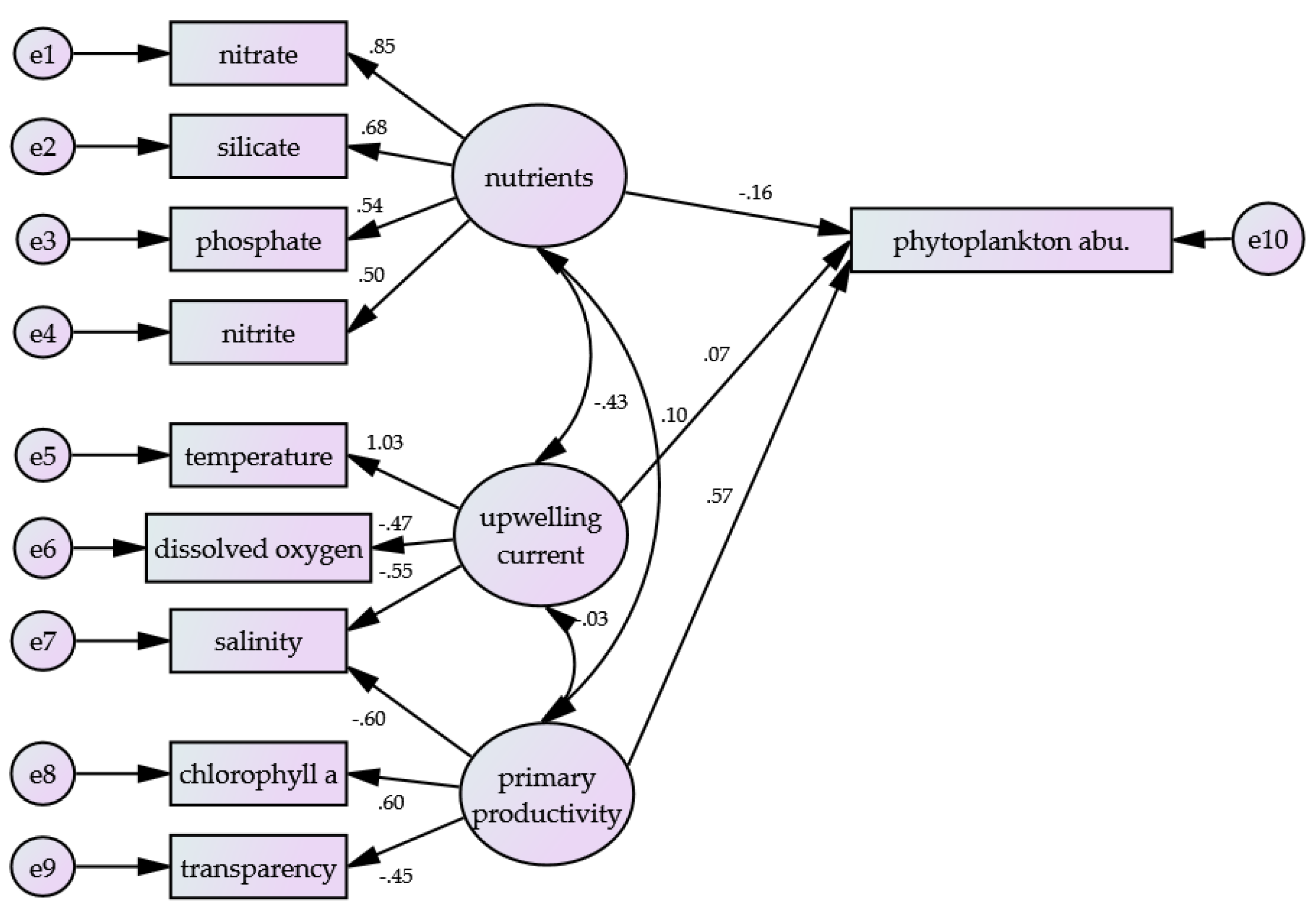
3.4.1. Water Quality Environmental Factors and Phytoplankton Cluster

Figure 3 shows the structural pattern between water quality environments and phytoplankton cluster. The RMSEA (0.113) fell within the “bad fit” range, indicating that the setting of the study model was not effectively matched with the sampling data. Additionally, the rest of the indicators did not meet the reference criteria. Hence, the overall model did not pass the test.

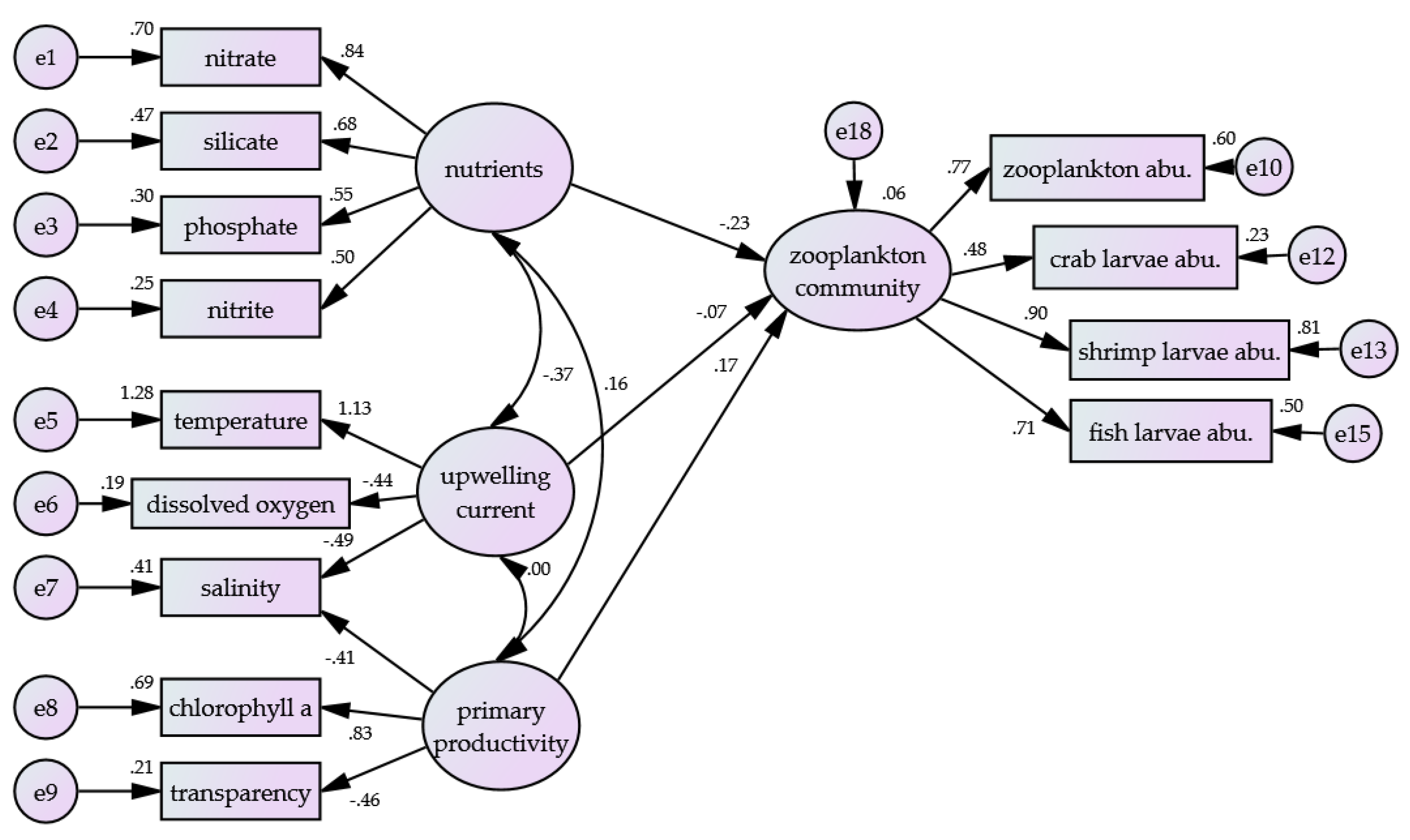
3.4.2. Water Quality Environmental Factors and Zooplankton Cluster

Figure 4 shows the structural pattern between water quality environments and the zooplankton cluster. The RMSEA (0.085) value obtained from the model fit analysis (0.085) fell within the range of “moderately fit”, albeit falling short of the optimal reference value of less than 0.05. However, the obtained value was still considered acceptable, suggesting that the conceptual model proposed was in line with the empirical data obtained. Meanwhile, the non-normed fit index (NNFI) value (0.842) did not meet the reference criteria, which was used to assess the degree of association between the research model and the observed variables, and to identify areas for model improvement. Hence, adjustment is needed for covariate relationships.

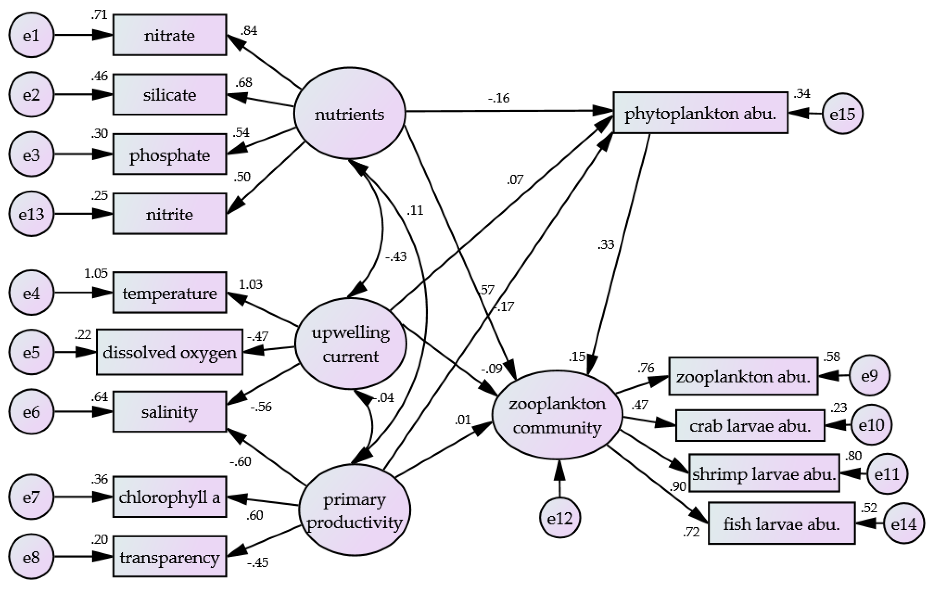
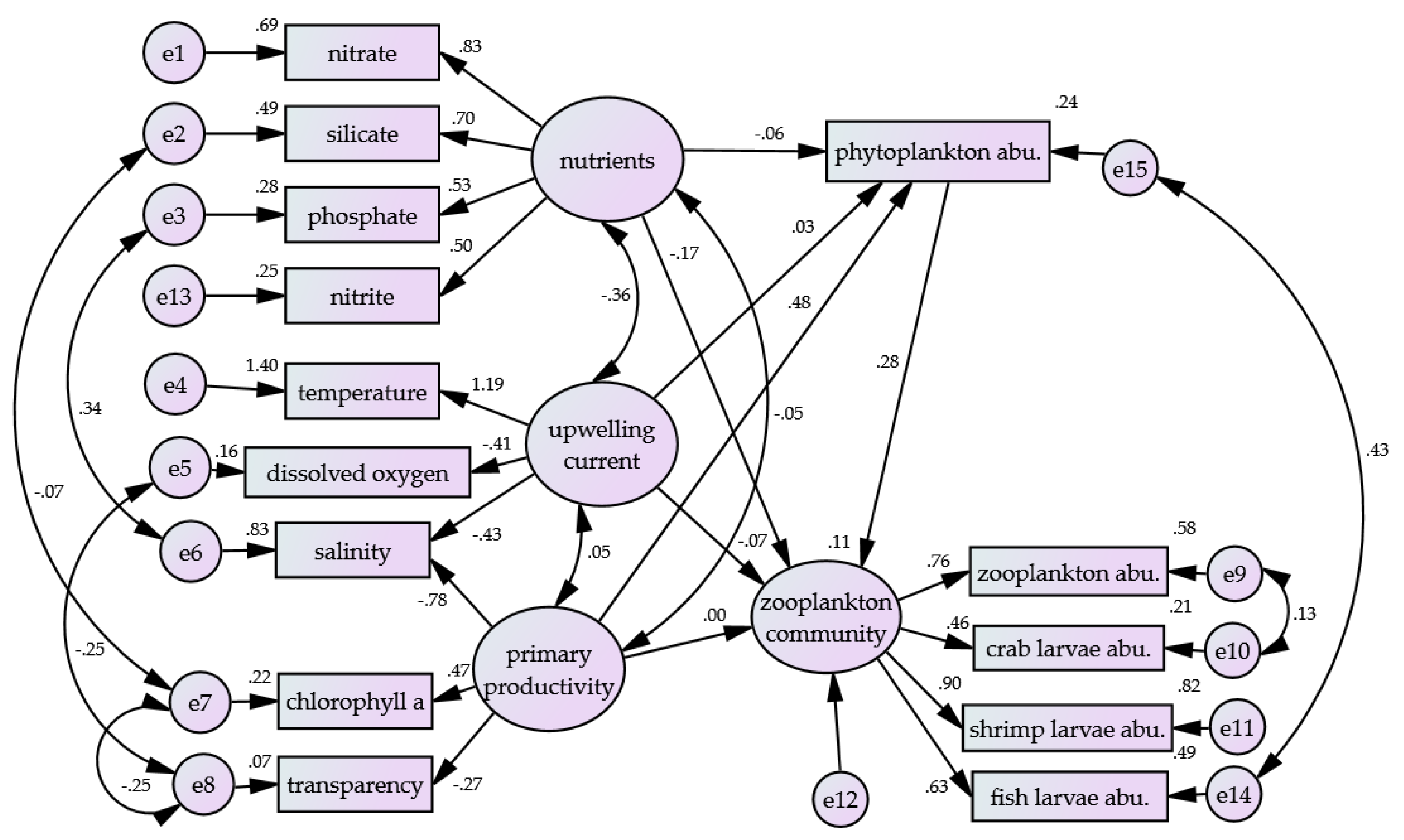
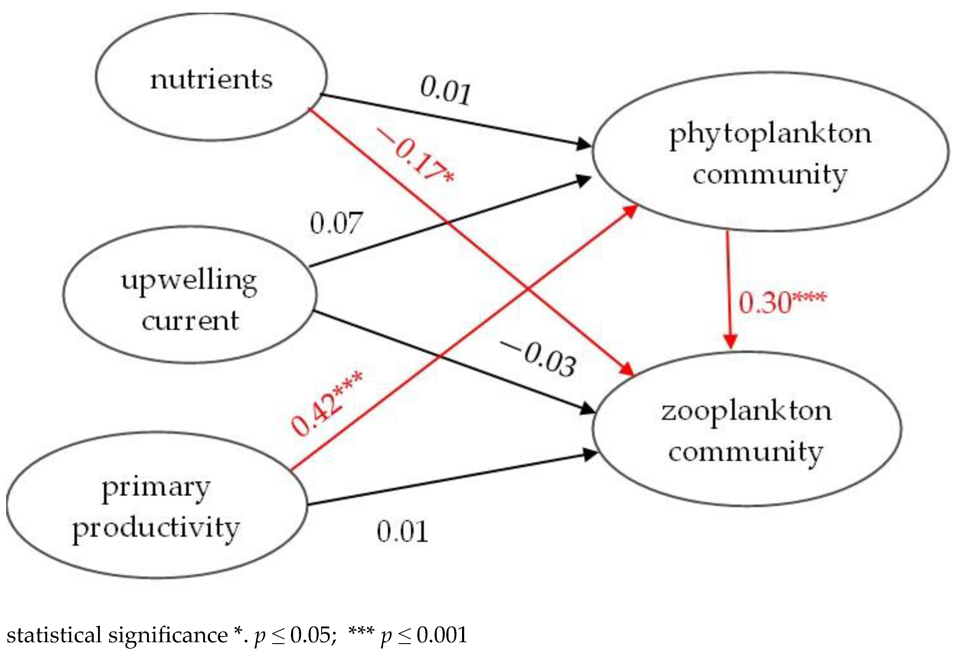
3.4.3. Water Quality Environmental Factors and Plankton Cluster

Figure 5 presents the structural pattern between water quality environments and both phytoplankton and zooplankton clusters. The RMSEA index displayed a value of 0.097, which indicates a “moderate” fit; however, it was close to the threshold of a poor fit. This suggested that the model and the sampling data had only a low probability of effectively explaining the results. Furthermore, the NNFI value (0.787) did not meet the reference criteria. The GFI value (0.892) also failed to meet the reference criteria. GFI is primarily used to test the proportion between the variance of the explainable observed variables before model adjustment and covariance. On the other hand, AGFI (0.831) met the criteria, suggesting the need for more observational data to enhance the interpretation of the observed and potential variables in the model.

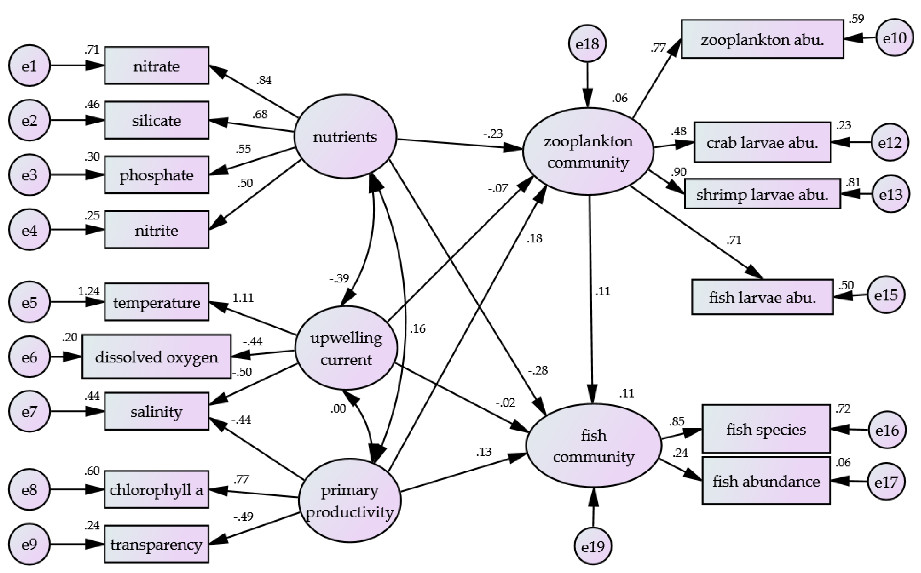
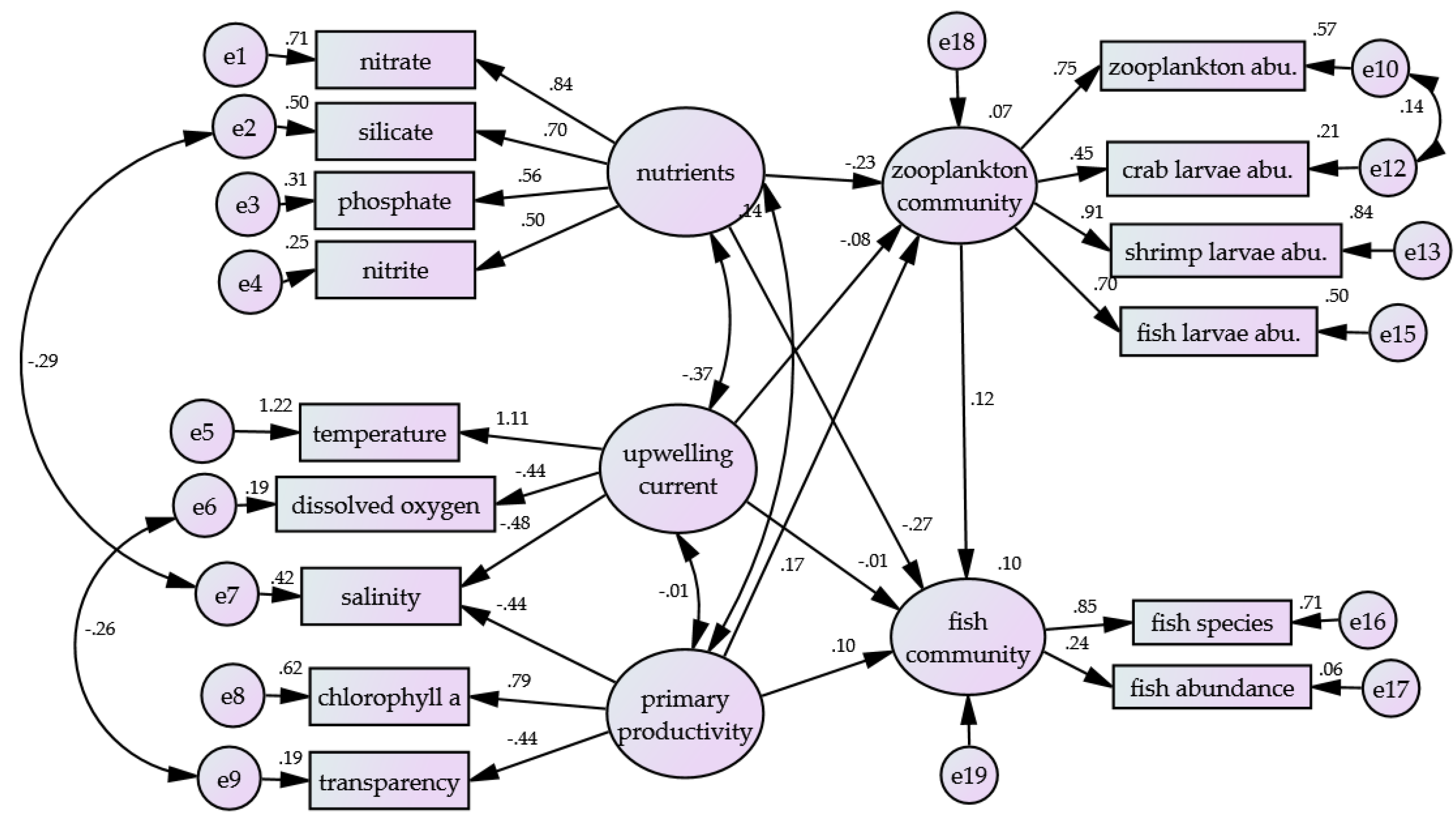
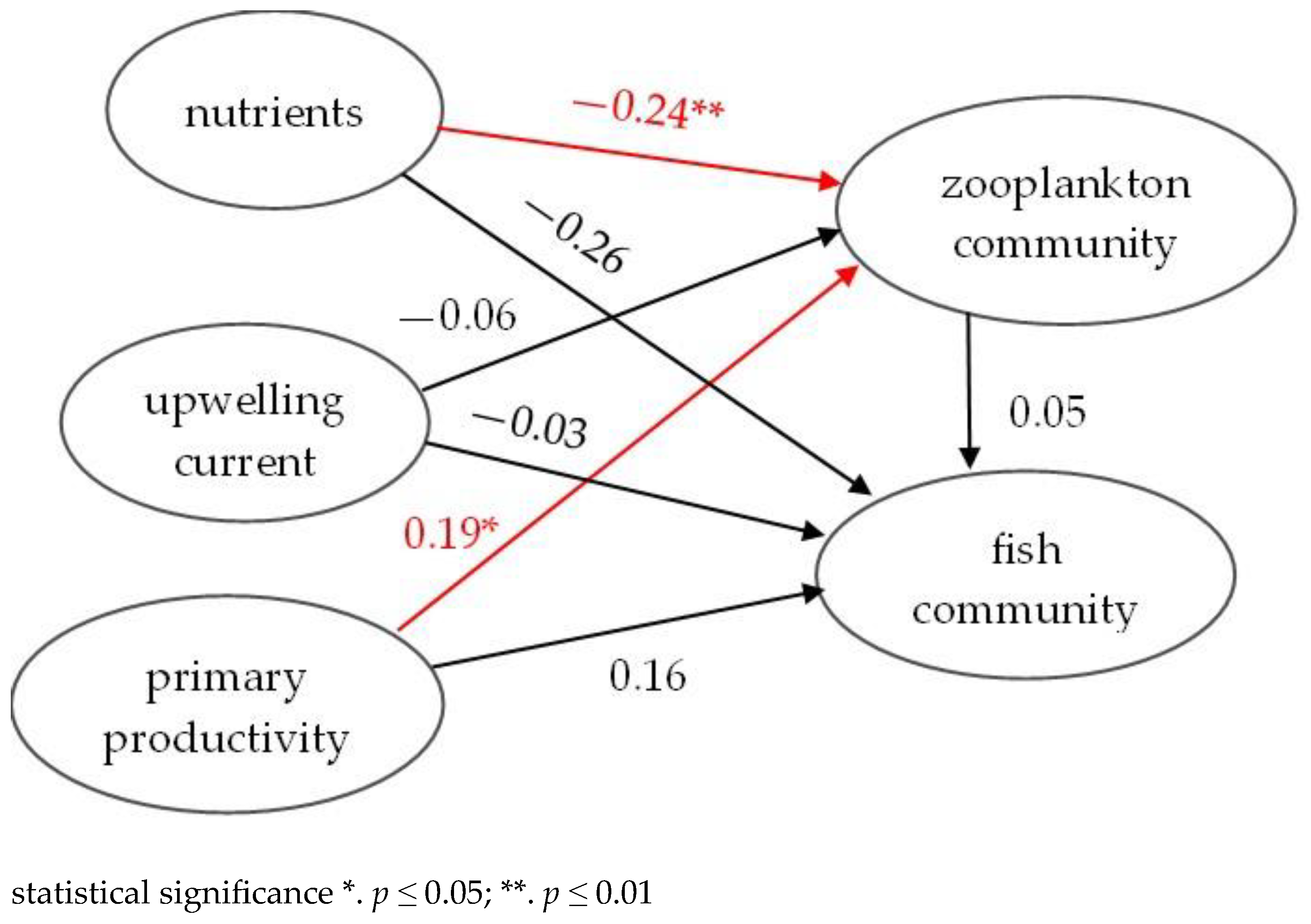
3.4.4. Water Quality Environmental Factors and Marine Life Cluster

The structure that included all three clusters was also considered. However, due to the high correlation between chlorophyll a and the phytoplankton cluster, we reserved chlorophyll a to represent the primary productivity and dropped the phytoplankton cluster.

Figure 6 shows the comprehensive structure pattern between water quality environments and both zooplankton and fish clusters. Of all the indices utilized, only NNFI (0.840) fell short of meeting the reference value, therefore, requiring the further refinement of the model. The remaining indices successfully passed the test, with RMSEA (0.074) reaching a level of good fit. This suggested that the model has the potential to effectively explicate marine ecological phenomena to a significant extent.

This model which examined the relationship between environmental factors and marine life clusters failed to meet the NNFI criteria. This outcome may be attributed to several factors, including the nature of the sample itself; environmental changes, such as seasonal and weekly–daily fluctuations; and the accuracy and stability of the measuring instrument. These factors may result in a higher probability of standard errors (non-normal distribution) in the measurement variables. Furthermore, various potential environmental factors in Nanway Bay, such as sea tides and internal wave phenomena, were not included in the statistical analysis. Consequently, the proposed model may be limited in its ability to explain ecological phenomena solely within the sampled waters and may not be applicable to other water bodies.

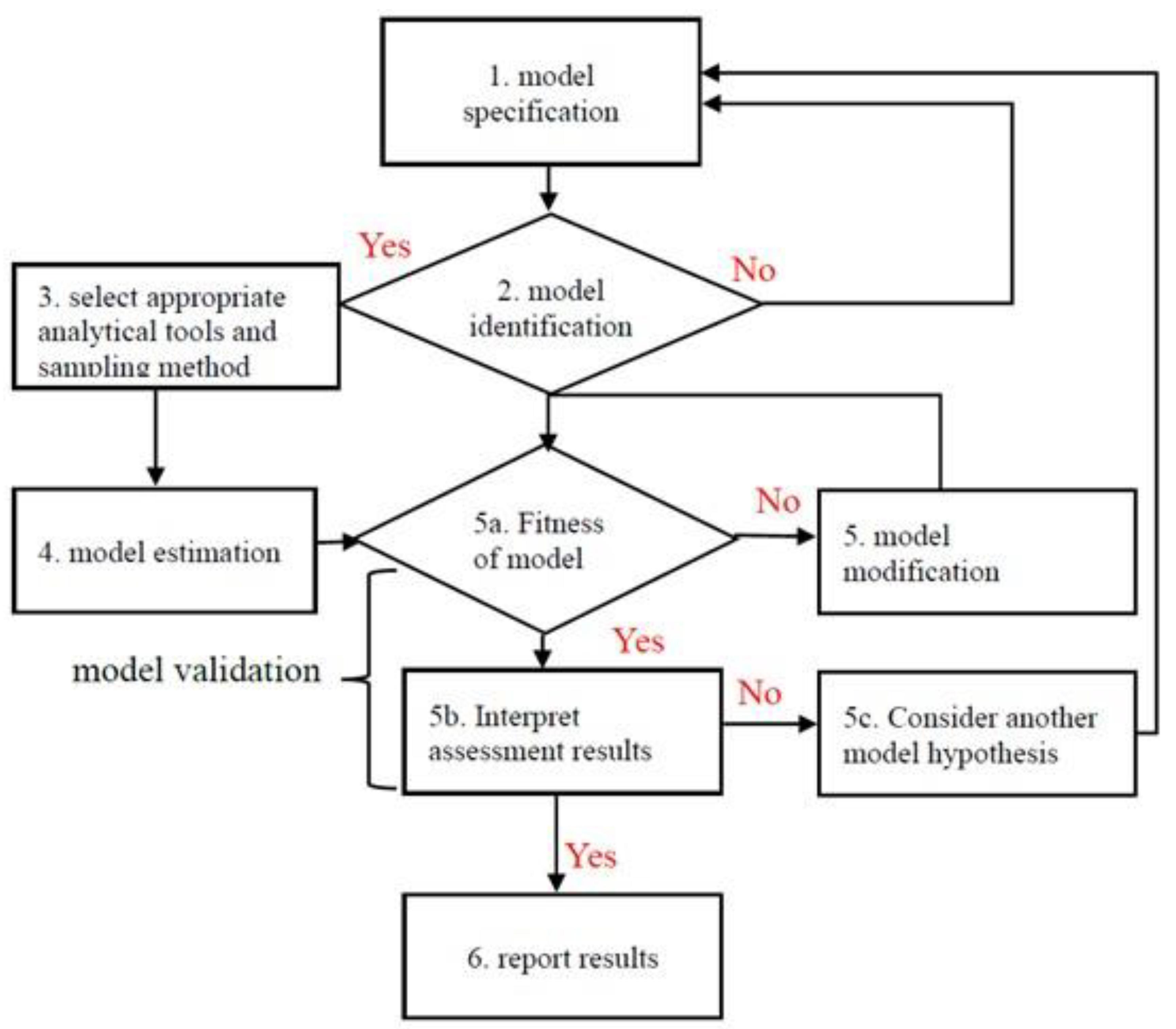
3.5. Model Modification

Continuing with the results of the model verification, the next step involved model modification. Due to the covariant relationship between the observed variables in the model, parameters in the modification index (MI) provided in the Amos Graphics software could be used to modify the model. The main objectives of model modification were to improve its simplicity, model fit, explanatory power, and reduce measurement error and structural residuals. However, there was a risk of losing the characteristic of verification and converting the model into an exploratory tool. In the context of the measurement model, one way to modify the model is to allow correlation between measurement variables when supported by theory or the literature.

The objective of this study was to explore the correlation between the variables presented in Figure 5 and Figure 6. During the model verification phase, the root mean square error of approximation (RMSEA) of the models, shown in Figure 4, Figure 5 and Figure 6, were all in the moderate fit range (0.08 to 0.10). Notably, the model depicted in Figure 6 achieved a better fit range (0.05 to 0.08). As the correlation of the variables in the model of Figure 4 was included in the model of Figure 5, only the models in Figure 5 and Figure 6 were considered for revision.

The model in Figure 5 was modified based on the MI value provided in the Amos report by establishing the correlation between the residuals of measured variables. Specifically, the correlation between measured variable residuals was increased to reduce the Chi-square value, following the principle of modifying one parameter at a time. The revised model is shown in Figure 7. After the revision, the NNFI (0.939) was in accordance with the reference criteria, and the rest of the indices also provided validation for the model; RMSEA (0.052), especially, reached the well-fit range, indicating that the model and observed data achieved the desired fit (

Table 9. The model evaluation results of the modified SEM of environmental variables and the plankton clusters.

Key Metrics	Reference Guidelines	Model Validation	Test Results
χ2	The lower the better	97.663
χ2/df	<5(<3 better fit)	1.601	Compliant
GFI	>0.9	0.941	Compliant
AGFI	>0.9(>0.8 acceptable fit)	0.898	Compliant
RMSEA	<0.05, good fit	0.052	Reasonable fit
	0.05~0.08, reasonable fit
	0.08~0.10, medium fit
	>0.10, poor fit
SRMR	≤0.08	0.0634	Compliant
NNFI	>0.9	0.939	Compliant
PNFI	≥0.5	0.604	Compliant
PGFI	≥0.5	0.547	Compliant
GN	≥200	223	Compliant

).

Figure 8 is the revision of Figure 6, and the results are shown in

Table 10. The model evaluation results of the modified SEM of environmental variables and marine life.

Key Metrics	Reference Guidelines	Model Validation	Test Result
χ2	The lower the better	127.053
χ2/df	<5(<3 better fit)	1.672	Compliant
GFI	>0.9	0.931	Compliant
AGFI	>0.9(>0.8 acceptable fit)	0.891	Compliant
RMSEA	<0.05, good fit	0.055	Reasonable fit
	0.05~0.08, reasonable fit
	0.08~0.10, medium fit
	>0.10, poor fit
SRMR	≤0.08	0.0621	Compliant
NNFI	>0.9	0.912	Compliant
PNFI	≥0.5	0.623	Compliant
PGFI	≥0.5	0.589	Compliant
GN	≥200	223	Compliant

. Notice that the normalized fit index (NNFI) attained a value of 0.912, satisfying the established reference criteria. Furthermore, the other indices also provided validation of the model, with particular emphasis on RMSEA, which fell within the well-fit range at 0.055. This indicated that the model and the observed data achieved the desired level of fit.

Upon completion of the model revision, a subsequent path analysis and the effect between variables were conducted to verify the assumptions made in this study.

3.6. Path Analysis

In addition to evaluating the overall fitness of the model modification and the intrinsic quality of the test, further examination was required to comprehend the linear association between the latent variables. This can be achieved through the observed direct effects and indirect effects to determine the direct and indirect impacts, as well as overall impacts (direct and indirect effects) among the latent variables.

The path relationships between facets were estimated using the structural equation model. Standardized coefficients were used to determine the relationship between the latent variables in the model, as depicted in Figure 7 and Figure 8. In Figure 9, the path effects of “nutrient on zooplankton clustering,” “primary productivity on phytoplankton clustering”, and “phytoplankton clustering on zooplankton clustering” were found to be statistically significant. Similarly, in Figure 10, the path effects of “nutrient on zooplankton clustering” and “primary productivity on zooplankton clustering” were also significant, indicating that both models possessed considerable predictive capabilities for assessing direct and indirect effects (enhancement or offset) on environmental and biological factors.

The path analysis provides empirical evidence of the direct and indirect effects. The direct effects of nutrients on the zooplankton cluster, primary productivity on the phytoplankton cluster, and phytoplankton cluster on the zooplankton cluster were found to be statistically significant (H2, H5, and H7, respectively). Additionally, the direct effects of nutrients on the zooplankton cluster and primary productivity on the zooplankton cluster were also statistically significant (H8 and H12, respectively). Among the significant direct effects, the effect of primary productivity on the phytoplankton cluster (H5) was the strongest (0.421).

In addition to the direct effects, the study also examined the indirect effects of the predictor variables on the zooplankton cluster. The results in

Table 11. The effects of environmental factors and plankton cluster.

		Phytoplankton	Zooplankton
Nutrients	Direct effect	0.009 (H1)	−0.172 * (H2)
	Indirect effect	-	0.003
	Total effect	0.009	−0.169
Upwelling Current	Direct effect	0.072 (H3)	−0.033 (H4)
	Indirect effect	-	0.0231
	Total effect	0.072	−0.012
Primary Productivity	Direct effect	0.421 *** (H5)	0.012 (H6)
	Indirect effect	-	0.122
	Total effect	0.421	0.135
Phytoplankton	Direct effect	-	0.290 *** (H7)
	Indirect effect	-	-
	Total effect	-	0.290

* p < 0.05; *** p < 0.001; different superscripts indicate significant difference.

and

Table 12. The effects of environmental factors and marine life.

		Zooplankton	Fish Species
Nutrients	Direct effect	−0.239 ** (H8)	−0.265 (H9)
	Indirect effect	-	−0.011
	Total effect	−0.239	−0.276
Upwelling Current	Direct effect	−0.056 (H10)	−0.034 (H11)
	Indirect effect	-	−0.003
	Total effect	−0.056	−0.036
Primary Productivity	Direct effect	0.192 * (H12)	0.159 (H13)
	Indirect effect	-	0.006
	Total effect	0.192	0.168
Zooplankton	Direct effect	-	0.048 (H14)
	Indirect effect	-	-
	Total effect	-	0.048

* p < 0.05; ** p < 0.01; different superscripts indicate significant difference.

indicated that, except for the path of primary productivity on the zooplankton cluster, which had a rather higher coefficient of 0.122, the remaining paths had lower coefficients. Therefore, the direct effects were found to be more significant than the indirect effects.

Notably, despite being presented as a latent variable in the SEM model, the upwelling current did not display any direct or indirect effects on plankton and fish assemblages in Nanwan Bay. It is worth mentioning that areas characterized by upwelling currents are commonly known to provide ideal fishing grounds due to the abundant nutrient supply for planktonic communities [28]. Therefore, it is plausible that the upwelling current may indirectly influence other environmental factors, such as nutrient availability and primary productivity, which in turn have an impact on the distribution and abundance of phytoplankton, zooplankton, and fish.

Overall, the study suggested that the marine environment was subject to various factors that may influence the relationships between nutrient salt, primary productivity, phytoplankton cluster, and zooplankton cluster. This may explain why the indirect effects were not significant in this study. It is also possible that there were other intermediary variables or relationships that were not included in the structural statistics, or that the data themselves had a high degree of variation.

4. Conclusions

Our investigation aimed to unravel the intricate connections between environmental factors and marine life in Nanwan Bay. By employing structural equation modeling (SEM), we uncovered significant findings that illuminated the complex dynamics within the bay’s marine ecosystem. These insights provide valuable contributions to our understanding of the relationships and dependencies among environmental factors and the organisms inhabiting Nanwan Bay.

The first notable finding emerged from the modified models developed in this study, namely “modification of environmental factors and plankton clusters” and “modification of environmental factors and marine life clusters”. These models identified “primary productivity” and “nutrient” as the main environmental change factors, with a considerable degree of impact on the abundance and distribution of plankton clusters. Notably, the analysis revealed that primary productivity exhibited the highest direct effect on plankton clusters, emphasizing its pivotal role in shaping plankton communities.

Building upon the findings from the modified models, the second finding explored the relationship between the upwelling current and the phytoplankton cluster, zooplankton cluster, and fish cluster. Surprisingly, the path analysis indicated that the upwelling current did not have a statistically significant effect on these variables. This suggests that the direct impact of the upwelling current on the studied marine organisms might be limited, despite playing a role in the SEM models.

The proposed SEM offers valuable insights into the intricate relationships between environmental factors and marine organisms, particularly in the context of water quality, plankton communities, and fish populations. The findings highlight the significant influence of primary productivity and nutrients while also providing a nuanced understanding of the role of the upwelling current in the study area.

References

1. Doney, S.C.; Duffy, J.E.; Barry, J.P.; Chan, F.; English, C.A.; Galindo, H.M.; Grebmeier, J.M.; Hollowed, A.B.; Knowlton, N.; Polovina, J.; et al. Climate Change Impacts on Marine Ecosystems. Annu. Rev. Mar. Sci. 2012, 4, 11–37. [Google Scholar] [CrossRef] [Green Version]
2. Colebrook, J.M. Continuous plankton records: Seasonal variations in the distribution and abundance of plankton in the North Atlantic Ocean and the North Sea. J. Plankton Res. 1982, 4, 435–462. [Google Scholar] [CrossRef]
3. Ramdani, M.; Elkhiati, N.; Flower, R.J.; Thompson, J.R.; Chouba, L.; Kraiem, M.M.; Ayache, F.; Ahmed, M.H. Environmental influences on the qualitative and quantitative composition of phytoplankton and zooplankton in North African coastal lagoons. Hydrobiologia 2009, 622, 113–131. [Google Scholar] [CrossRef]
4. Wei, X.-Y.; Wang, Y.-C.; Zhang, K.; Dang, Y.-Q.; Xiong, X.-W.; Shang, Z. Review of assessment of thermal discharges from power plants on aquatic biota. J. Hydroecology 2018, 39, 1–10. [Google Scholar]
5. Poornima, E.H.; Rajadurai, M.; Rao, T.S. Impact of thermal discharge from a tropical coastal power plant on phytoplankton. J. Therm. Biol. 2005, 30, 307–316. [Google Scholar] [CrossRef]
6. Jiang, Z.B.; Zeng, J.N.; Chen, Q.Z. Potential impact of rising seawater temperature on copepods due to coastal power plants in subtropical areas. J. Exp. Mar. Biol. Ecol. 2009, 368, 196–201. [Google Scholar] [CrossRef]
7. Marrasse, C.; Lim, E.; Caron, D. Seasonal and daily changes in bacterivory in a coastal plankton community. Mar. Ecol. Prog. Ser. 1992, 82, 281–289. [Google Scholar] [CrossRef]
8. Cooke, S.J.; Bunt, C.M.; Schreer, J.F. Understanding fish behavior, distribution, and survival in thermal effluents using fixed telemetry arrays: A case study of smallmouth bass in a discharge canal during winter. J. Environ. Manag. 2004, 33, 140–150. [Google Scholar] [CrossRef] [PubMed]
9. Chen, C.-T.A.; Tsai, H.-S.; Lin, W.-H.; Wang, B.-J.; Lui, H.-K. Hydrology and water chemistry around the Third Nuclear Power Plant dominated by large scale environmental changes. Mon. J. Taipower’s Eng. 2016, 810, 64–71. [Google Scholar]
10. Chen, C.-T.A.; Jan, S.; Chen, M.-H.; Liu, L.-L.; Huang, J.-F.; Yang, Y.-J. Far-field influences shadow the effects of a nuclear power plant’s discharger in a semi-enclosed bay. Sustainability 2023, 15, 9092. [Google Scholar] [CrossRef]
11. Pugesek, B.H.; Tomer, A.; von Eye, A. Structural Equation Modeling: Applications in Ecological and Evolutionary Biology; Cambridge University Press: Cambridge, UK, 2003; 336p. [Google Scholar]
12. Jia, L.; Shen, L.; Shuai, C.; He, B. A novel approach for assessing the performance of sustainable urbanization based on structural equation modeling: A China case study. Sustainability 2016, 8, 910. [Google Scholar] [CrossRef] [Green Version]
13. Kaiser, H.F. An index of factorial simplicity. Psychometrika 1974, 39, 31–36. [Google Scholar] [CrossRef]
14. Chen, S.-Y. Multivariate Analysis, 4th ed.; Huatai Book Company: Taipei, China, 2005; 710p. [Google Scholar]
15. Hwang, F.-M. The Statistical Methodology for Social Science-Structural Equation Modeling; Wunan Bookstore: Taipei, China, 2004; 477p. [Google Scholar]
16. Hwang, F.-M. Structural Equation Modeling; Wunan Bookstore: Taipei, China, 2009; 496p. [Google Scholar]
17. Hair, J.F., Jr.; Anderson, R.E.; Tatham, R.L.; Black, W.C. Multivariate Data Analysis, 5th ed.; Englewood Cliffs: Prentice-Hall, NJ, USA, 1998; 730p. [Google Scholar]
18. Carmines, E.G.; McIver, J.P. Analyzing Models with Observable Variables. In Social Measurement; Bohrnstedt, G.W., Borgatta, E.F., Eds.; Sage: Beverly Hills, CA, USA, 1981; pp. 65–115. [Google Scholar]
19. Joreskog, K.G.; Sorbom, D. LISREL 8: User’s Reference Guide; Scientific Software International: Chicago, IL, USA, 1996; 378p. [Google Scholar]
20. Hair, J.F.; Black, W.C.; Babin, B.J.; Anderson, R.E.; Tatham, R.L. Multivariate Date Analysis, 6th ed.; Pearson Education, Inc.: London, UK, 2006; 899p. [Google Scholar]
21. Browne, M.W.; Cudeck, R. Alternative Ways of Assessing Model Fit. In Testing Structural Equation Models; Bollen, K.A., Long, J.S., Eds.; Sage: Newbury Park, CA, USA, 1993; pp. 136–162. [Google Scholar]
22. Hu, L.; Bentler, P.M. Cutoff criteria for fit indexes in covariance structure analysis: Conventional criteria versus new alternatives. Struct. Equ. Model. 1999, 6, 1–55. [Google Scholar] [CrossRef]
23. Tucker, L.R.; Lewis, C. A reliability coefficient for maximum likelihood factor analysis. Psychometrika 1973, 38, 1–10. [Google Scholar] [CrossRef]
24. Mulaik, S.A.; James, L.R.; Van Alstine, J.; Bennet, N.; Lind, S.; Stilwell, C.D. Evaluation of Goodness-of-Fit Indices for Structural Equation Models. Psychol. Bull. 1989, 105, 430–445. [Google Scholar] [CrossRef]
25. Walsh, J.J.; Whitledge, T.E.; Esaias, W.E.; Smith, R.L.; Huntsman, S.A.; Santander, H.; De Mendiola, B.R. The spawning habits of the Peruvian anchovy, Engraulis ringens. Deep Sea Res. 1980, 27, 1–27. [Google Scholar] [CrossRef]
26. Armstrong, D.A.; Mitchell-Innes, B.A.; Verheye-Dua, F.; Waldron, H.; Hutchings, L. Physical and biological features across an upwelling front in the southern Benguela. S. Afr. J. Mar. Sci. 1987, 5, 171–190. [Google Scholar] [CrossRef]
27. Longhurst, A.R.; Pauly, D. Ecology of Tropical Oceans; Academic Press: London, UK, 1987; 407p. [Google Scholar]
28. Otero, J.; Álvarez-Salgado, X.A.; Bode, A. Phytoplankton diversity effect on ecosystem functioning in a coastal upwelling system. Front. Mar. Sci. 2020, 7, 592255. [Google Scholar] [CrossRef]
Figure 1. The location of research geography and sampling stations. ● Sampling station of water quality and plankton; ▲ Sampling station of fish.
Sustainability 15 11435 g001
Figure 2. The construction process of SEM.
Sustainability 15 11435 g002
Figure 3. SEM of environmental variables and the phytoplankton cluster.
Sustainability 15 11435 g003
Figure 4. SEM of environmental variables and the zooplankton cluster.
Sustainability 15 11435 g004
Figure 5. SEM of environmental variables and plankton clusters.
Sustainability 15 11435 g005
Figure 6. SEM of environmental variables and marine life.
Sustainability 15 11435 g006
Figure 7. Modified SEM of environmental variables and plankton clusters.
Sustainability 15 11435 g007
Figure 8. Modified SEM of environmental variables and marine life.
Sustainability 15 11435 g008
Figure 9. The path analysis of environmental variables and plankton clusters.
Sustainability 15 11435 g009
Figure 10. The path analysis of environmental variables and marine life.
Sustainability 15 11435 g010