Modeling and Analysis of the Impact of Risk Culture on Human Behavior during a Catastrophic Event

Abstract

In a world more and more affected by natural and/or industrial disasters, it is essential to understand, analyze and control human behavior during such events. The work presented in this article is one of the results of a transdisciplinary collaboration between geographers, psychologists, mathematicians, computer scientists, operational staff and stakeholders in risk management. This collaboration made it possible to identify the diverse behavioral reactions that can occur during a disaster and to propose a categorization of these behavioral states and their transitions. These behavioral dynamics are described by the APC (Alert–Panic–Control) mathematical model, which integrates two key elements (among others) during disasters: cognition and social contagion. Several scenarios are developed, and a qualitative analysis of the model is conducted to better understand the role of crowd density and risk culture on behavioral dynamics.

1. Introduction

The last decades have been marked by a sharp increase in the number of disasters with a clear decrease in human losses and a strong increase in financial losses. This observation, particularly noticeable in developed countries, is a source of optimism. But new risks are constantly being announced for the future, and some of them might develop into disasters, or even crises. They could concern cyberculture, biotechnologies, pandemics, various forms of urban terrorism and climate change [1]. A risk-free society is therefore not to be expected anytime soon. If the future does not seem much more encouraging than the close past, there is no reason to be alarmist, as Western societies sometimes seem to be. On the contrary, it is all the more important to expand our understanding of the reality of a risk or disaster and of how to anticipate and manage them [2,3,4] but also of how people react to them [5,6,7,8,9]. This reaction is the main focus of research today. What do we know about the human reactions of individuals and populations during disasters? Knowledge is still limited, except for the fact that forms of collective panic have been observed and transcribed during natural, technological, and health disasters [10,11,12,13] even though this has given rise to sometimes heated debate between different scientific communities [14,15,16]. Now that national and regional officials are legally responsible for incidents caused by the management of crowds and large gatherings, these panic reactions are even more feared by those in charge of responding to disasters that cannot be easily managed because they are triggered and spread like wildfire. Panic behaviors alone are not sufficient to describe these collective behaviors. Controlled behaviors have also been reported [17,18,19]: some reflect static reactions such as immobility and bewilderment; others reflect dynamic reactions such as deliberate flight, exit or even mutual aid [20,21,22]. Finally, research in psychology and neuroscience has suggested that human beings rarely remain frozen in a single behavioral state but go through a chain of reactions from the beginning to the end of a disaster.

When individuals adapt their behavior to a disaster, they become less vulnerable and prevent a fatal situation of collective panic. This is particularly true during sudden and unforeseen disasters where it is impossible to deploy crisis management staff in the field before the occurrence of the event. In this context, policies in France and Europe for preventing and managing risks and disasters that initially focused on actions and strategies aimed at mitigating or even eliminating hazards and threats now aim at “helping citizens to be active in ensuring their own safety”(in France: civil protection modernization act no. 2004-811 of 13 August 2004). To be active in ensuring their own safety means to adapt their behavior to the disaster that is occurring and to do so as ordinary citizens when faced with an exceptional event and not as persons trained to respond to uncertainty and emergencies. Hence the first question to which we will suggest possible answers: How can citizens be prepared to adopt the most appropriate behavior(s) during a disaster that occurs suddenly and unexpectedly? To answer this first question, the concept of risk culture is usually brought into play. Our objective will be to determine the potential impact of the risk culture on the emergence and potentially the dissemination of controlled collective behaviors rather than collective panic behaviors. The second question linked to the first is how to identify the diverse behaviors, the temporal patterns specific to each of them, and the changes from one behavioral state to the other—that is, how several reactions are linked together to deal with a disaster. Our objective is to model these behavioral dynamics.

To answer these different questions and meet these objectives, a highly interdisciplinary collaboration has been developed within the Com2SiCa research project, whose aim is to understand and simulate human behavior in disaster areas. This research project involves both academics (geographers, psychologists and mathematicians specialized in modeling risks, disasters, and human behavior in these situations of uncertainty) and governmental and non-governmental operational staff involved in managing crises and disasters such as emergency response teams on site that ensure the protection of the population and their safety(rescue service)-, and the local officials in charge of crisis management or of major risk prevention (Prefecture of the Alpes-Maritimes, Departmental Directorate of Territories and the Sea of the Alpes-Maritimes, Departmental Fire and Rescue Service of the Alpes-Maritimes, Paris Fire Brigade, National Police, Municipal Police of Nice, Regional Health Agency, the Major Risks Department of the Nice Côte d’Azur Metropolis and city of Nice, the Major Risks Department of Le Havre Seine Métropole Urban Community, National Union of Communal Social Action Centers). More details are available at https://www.com2sica.cnrs.fr/ (accessed on 11 July 2023).

Effective collaboration is particularly essential because operational staff and policymakers in charge of risk management must deal with situations that involve many complex interaction systems that are difficult to dissociate. The geography of risks serves to better identify and understand these different interaction systems (behaviors, spatial constraints, etc.), and mathematical models can reconstruct situations in which these different interaction systems can be dissociated to gain a better understanding of them. The co-constructed models thus enrich our knowledge of these complex processes and enlighten politicians in their decision making. Supplementary information about this interdisciplinary cooperation and the research background can be found in [1,22,23].

The models that we have developed here disregard the dynamics of collective pedestrian movements [24,25,26,27,28,29,30] and focus on aspects that were often less detailed in the previous models: the modeling of behavioral states, the way they evolve during a disaster, and the phenomena of social propagation of these states which we summarize under the name of behavioral dynamics. Note that if spatial configurations have an impact on these behavioral dynamics [1,31,32,33,34] previously studied in [35], we are not taking them into account in this paper, which only focuses on the impact of risk culture on these dynamics.

Two scales can be used to model behavioral dynamics and interactions: the individual level (a micro-approach that usually uses agent-based models) and the collective level (a macro-approach that usually uses models based on dynamical systems) (see Figure 1).

In micro- or agent-based models [27,36,37] a degree of randomness must be introduced in the behavior of individuals; behaviors assigned to individuals cannot therefore be fully justified scientifically. These models give the appearance of great precision, and yet they allow a very large degree of freedom that prevents any control of the dynamics, which is needed to understand the processes that generate them. Because of these limitations, we did not use this type of modeling to analyze collective behavioral dynamics in disaster situations, since the objective of policies and notably of risk policies is to manage and regulate situations at the collective level and not to manage each individual. We therefore selected a model based on dynamical systems with parameter settings suited to this management scale. The tools and laws defined within the framework of a risk policy are intended for the entire population, and they act on a macroscopic scale. They are then adopted or not by each person (see Figure 2). What policymakers need to know is precisely whether these actions (laws, regulations, etc.) collectively modify behavior and reduce the vulnerability of populations by raising their awareness about risks. This is why the proposed macroscopic models are useful decision-making tools for operational staff. In addition, these models integrate available knowledge about the collective properties of a population and about the process(es) involved in a disaster without needing quantitative data. Indeed, models based on ordinary differential equations (ODEs) are built with parameters well suited to the actions of operational staff, which are actions intended for a group and not for individuals. For example, the simple, continuous modification of a parameter considered important, in this case the risk culture parameter, is sufficient to deduce variations in collective human behavioral dynamics. These models therefore gather available knowledge about the emergency and can be used as a tool to train operational staff and develop our understanding of the emotional behavior of individuals that can lead to panic, among other reactions.

Starting from 2014, a few studies based on epidemic macroscopic models have appeared in the literature in order to investigate the propagation of emotions in a population. An SIRLS (Susceptible–Infected–Recovered–Latent–Susceptible) model was developed to study the propagation and control of panic emotions in a population during emergencies [38]. More recently, a PCR model (Panic–Control–Reflex) [23,39] based on cognitive sciences and the mathematical modeling of infectious diseases was proposed to describe the different human behavioral dynamics during catastrophic events. Both approaches highlight the importance of taking into account the phenomenon of emotion contagion when modeling populations in disaster situations. The second, however, proposed by our consortium not only focuses on panic; it also presents an accurate analysis and classification of the behaviors depending on the different brain regions that are activated and the different behavioral transitions. This approach is based on a model inspired by neuroscience which may, however, be insufficient to describe the social interactions involved in behavioral changes.

In order to include both cognition and social contagion [40,41] in our modeling, these two aspects are understood from the perspective of emotional load and regulation [42], which leads to a richer mathematical model, the APC model (Alert–Panic–Control). Using the APC model proposed here, we studied the potential impact of risk culture on the different behaviors that can be adopted.

The paper is organized as follows. In Section 2, we present the different behavioral categories we consider in our study and we introduce the thematic hypotheses on the behavioral transitions based on this categorization and our data collections. Section 3 proposes the APC model, a mathematical model based on nonlinear ODEs, that describes human collective behaviors in disaster situations. Section 4 develops a qualitative analysis of the model. For this analysis, we identify parameter values that reflect contexts with a dense or sparse population and different levels of risk culture. This analysis allows us to identify the parameter values that lead to the predominance of a panic or a controlled behavior.

2. Behavior Characterization

2.1. Behavioral Diversity Drawn from a Variety of Corpora

To grasp the full diversity and complexity of behavioral responses in disaster situations, we observed and analyzed these situations in different types of corpora used in the humanities and social sciences, namely: texts, audio and video material, and maps. These complementary corpora were used to collect and produce data drawn from real or simulated disasters.

2.1.1. Concerning the Collection of Data and Knowledge Regarding Human Behavior during Real Disasters

The textual and audio material was collected from governmental and non-governmental frontline responders on disaster scenes (terrorist attacks, wars, natural and industrial disasters, etc.). Their very presence in these locations makes them valuable witnesses, and their experience and knowledge are essential for research and for anticipating and managing major crises. Three focus group surveys (12 March 2018, 13 April 2018, 9 and 10 October 2018) and two workshops (5 November 2018, and 19 June 2019) were organized with crisis response teams from the Alpes-Maritimes and Seine-Maritime departments (France) participating in the Com2SiCa research program (to be more precise, the Alpes-Maritimes Departmental Fire and Rescue Service, the Prefecture of the Alpes-Maritimes, the Departmental Directorate of Territories and the Sea of the Alpes-Maritimes, the Paris Fire Brigade, the National Police, the Municipal Police of Nice, the Regional Health Agency, the Nice Côte d’Azur Metropolis and city of Nice for the Major Risks Department, Le Havre Seine Métropole Urban Community for the Major Risks Department, the National Union of Communal Social Action Centers). In addition to these sessions, a series of individual interviews were carried out during 2020 and 2021 with experts (emergency doctors, psychologists, first-aid responders, crisis managers) who often deal with major disasters. The persons interviewed included the founder of the national network of medical and psychological emergency units, the Paris Fire Brigade, the Alpes-Maritimes Departmental Fire and Rescue Service, and the Interministerial Crisis Management Operational Center. All these sessions (focus groups, workshops, and interviews) were recorded in full and supplemented by observation notes taken by the consortium researchers and photographs. The audio data recorded were then transcribed in full. In addition to the textual and audio material, a corpus of videos of close to forty major events belonging to the three major families of disasters (natural, technological, and societal) was also collected and analyzed to capture the diversity of human behaviors experienced on disaster scenes [22]. These videos were extracted from television reports, surveillance camera footage, videos recorded by response teams or posted on the Internet and on social networks. Once processed, these textual, audio and video corpora provided information on human behaviors observed on the actual scene of natural, technological, or societal disasters, on the categories of behavior that dominate in these scenes, and on the context (cultural, spatial, or environmental) that can influence behavior.

2.1.2. Concerning the Collection of Data and Knowledge Regarding Human Behavior during Simulated Disasters

We conducted immersive interviews with the population on actual sites in Nice in September 2018 and in Le Havre in May 2019 (individual 45-minute interviews with a total of 60 people surveyed on both sites). These protocols immersed participants in a sound and visual environment (a tsunami scenario of seismic origin in Nice and a technological accident scenario in Le Havre). Their behavioral reactions were then observed, recorded, and identified. The trajectories people followed to exit the imagined or projected situation were mapped, and the emotional load of each respondent was measured on a qualitative scale [43].

Recently promising possibilities have been offered by virtual computer-based experiments [44]. Our research team added an innovative protocol of virtual reality immersion to the experiments based on simulated situations [45]. The virtual reality immersion was carried out in a closed and controlled location at the Pays de la Loire Psychology Laboratory (Nantes) over the year 2020. It was based on the scenario of the arrival of a tsunami wave of seismic origin on a beach of Nice [46], which is a scenario that is now included in official French training material. The study more specifically analyzed the psychological, behavioral, and physiological reactions (physiological measures of stress) of participating volunteers. The scenario also included virtual characters (avatars) in order to allow researchers to observe reactions in a context of social interaction (between the volunteer and the virtual characters). The topographical data of the beach (width of the beach, presence of stairs, pebbles, access guardrails, etc.) was calibrated by precise measurements made during field surveys in Nice [45].

The processing of these different corpora provided the quantitative, qualitative, and spatial data used for the mathematical models (notably the types of behavior, changes in behavioral states and maps of movement trajectories).

2.2. Behavioral Categories

The diverse human behaviors were qualified and categorized into three behavioral states (alert, control and panic) identified by the analysis of the different corpora presented in Section 2.1 More than 60 human behaviors were identified. (Work on these results is in progress and has been recorded in internal reports communicated to the National Research Agency funding the project.) This categorization was achieved by using two important variables in emotional psychology: emotional charge or intensity (level of stress, nervousness, fear, etc.) and emotional regulation (the ability of people to control this charge) [47]. By crossing all these variables, we were able to qualify a wider range of responses or behaviors in disaster situations than panic only, as shown in Figure 3. Thus, we distinguish the following:

• Alert states (A) that designate a set of micro-behaviors that can be observed from physical movements (a startled expression, rapid eye movements, questioning people nearby verbally or with the eyes). The alert state corresponds to a phase of assimilation. It marks a break from ordinary behavior and corresponds to the very short time spent looking for information about the scenario the participant is experiencing. In the alert state, the person is in a state of uncertainty; the emotional charge is low even if some body signals may signal a break with the everyday behavior previously mentioned, such as for example an increased heartbeat rate.
• The controlled states or behaviors (C) are deliberate behaviors which designate a set of reactions with a more or less strong emotional charge that is regulated. Controlled behaviors are diverse: they can designate pro-social behaviors (mutual aid, protection, caring for others) but also anti-social behaviors (theft, looting, voyeurism, etc.). In other words, the notion of control designates the ability to regulate one’s emotions, to act and to adapt one’s behavior to the crisis context (it does not mean, however, that the behavior ensures the safety or survival of the person nor that it is virtuous, social, or exemplary with respect to a social norm).
• The set of panic behaviors (P) refers to uncontrolled behaviors dominated by fear-related emotions. Panic behavior implies a strong emotional charge and weak regulation, which is ineffective for regaining a controlled state. Different behaviors can reflect a panic state: panic flight, stupor, disorderly agitation [10].

These states were qualified by the intensity of the emotional charge and regulation, using the following approach:

• Alert states: low emotional charge and high emotional regulation.
• Controlled states: low or high emotional charge and high emotional regulation.
• Panic states: high emotional charge and low emotional regulation.

Furthermore, it is well known that during a disaster, human beings do not maintain the same behavior during the entire event. Instead, sequences of different reactions can be observed. For example, an alert state is adopted as soon as the event occurs. People then adopt a panic or controlled behavior depending on their past experience and risk culture.

Based on our categorization and in support of the analyses of the corpora presented in Section 2.1, we advance the following thematic hypotheses:

• The alert state can be very short and most often occurs at the very beginning of the event. However, depending on the characteristics of the event, if it is repeated as during earthquakes for example, the alert state may return, notably after a controlled state, but this is more rarely observed.
• An individual must pass through a controlled state to recover a pseudo-ordinary, everyday behavior which cannot be recovered as long as the person is in a panic state.
• We considered behavioral transitions according to two distinct processes: aggregation on one hand and imitation and propagation on the other. These processes, presented below, allow us to study the behavioral dynamics:

  -

  Intrinsic transitions linked to individual characteristics (age, experience, risk culture, etc.) and behaviors become collective by aggregation when a synchronization of individual behaviors occurs without necessarily any voluntary coordination or interaction among the group.

  -

  Transitions due to imitation and propagation, which allow us to understand the emergence of collective behaviors due to interaction within a population or a crowd. In some cases, the contagion processes can be caused by imitation, which is linked to a well-known phenomenon in social psychology, that is, social comparison [40]. The only behaviors that cannot be imitated are of the alert type. By nature, and because they are short, they cannot be imitated by populations in a panic or controlled state [48]. These propagation and imitation processes are used to study the dissemination of behaviors in time and space.

• Despite several interviews and focus groups carried out with a variety of persons who have experienced crises, knowledge is still uncertain regarding the changes in behavior linked to the presence of deceased people on a disaster scene. We therefore posit as a hypothesis that the impact of mortality on behavior does not create a feedback loop.

In the next section, we will build the APC mathematical model from these different thematic hypotheses.

3. Development of the Alert–Panic–Control Mathematical Model and Simulation of Behavioral Dynamics

Before going into the details of the APC model, we will first present what distinguishes it from the PCR mathematical model that the consortium had previously developed [39].

The PCR (Panic–Control–Reflex) model was based on a set of neurobiological responses to a threat, or a stress response, which is observed in the areas of the brain involved in these behavioral responses [49,50]. Two categories of behaviors were proposed: automatic, instinctive behaviors commanded by the reptilian brain, and acquired and controlled behaviors commanded by the prefrontal cortex. The first category includes the reflex behaviors of instinctive flight, panic, and bewilderment. The second category includes controlled or deliberate behaviors [23]. It should be noted that an automatic behavior does not mean that it is irrational. The fact that a reaction is automatic or instinctive does not imply that it is irrational, inappropriate, or wrong. The same applies to controlled behavior, which is not necessarily adapted to the situation. The PCR model was enriched by knowledge drawn from the psychology of emotions, as presented in Section 2. The new model proposed, known as the APC (Alert–Panic–Control) model, makes a distinction between states of Alert, Control, or Panic. As mentioned above, these states are qualified by the two key factors of emotion management that were selected: emotional charge or intensity (high or low) and emotional regulation (high or low) (see Figure 3).

With this new approach, data collected from observation and analysis of the surveys and experiments can be used to calibrate and constrain the mathematical model: that is, to define parameter ranges and orders of magnitude, and to validate sensitivity analyses. The sensitivity analysis, the identifiability study and the estimation of the parameters from the data collected were completed and are the subject of another study [51].

In this paper, we focus on presenting the model and designing realistic scenarios (Section 3) for studying the effects of population density and risk culture on behavioral dynamics (Section 4).

3.1. The APC Mathematical Model

The APC (Alert–Panic–Control) model we propose here is a compartmental model inspired by classical epidemic mathematical models such as the SIR (Susceptible–Infected–Recovered) one (see for example [52,53,54]). The APC model diagram is represented in Figure 4.

In this paper, we model the behavior of a population that experiences a sudden, rapid-onset catastrophic event without warning signs. We note $t_0$ as the initial moment of the event, and for $t\ge t_0$, according to the behavioral categories identified in Section 2.2, we introduce the following state variables:

• $a\left(t\right)$ is the density of population in a state of alert;
• $p\left(t\right)$ is the density of population in a state of panic;
• $c\left(t\right)$ is the density of population in a state of control.

In addition, we denote by

• $q\left(t\right)$ the density of population with an everyday behavior;
• $b\left(t\right)$ all the behaviors of everyday life after the disaster;
• $v\left(t\right)$ the density of the population that loses its life during the disaster.

We suppose that at the beginning, the entire population has an everyday behavior. Then, after the catastrophe is triggered (represented here by a function $\gamma$ defined later), people pass through a state of alert before adopting a panic or controlled behavior by an intrinsic reaction or an imitation process. A possible return to an alert behavior is also taken into account. In Figure 4, the intrinsic transitions are represented by solid lines, while the imitation processes are in dashed lines. The possible death of the three populations is considered. Finally, a return to an everyday behavior can only be achieved from a controlled behavior and only after a certain time (see the thematic hypotheses in Section 2.2). This transition is modeled by the function $\phi$ defined below.

Therefore, based on the transfer diagram of Figure 4, we present the first equation of the APC model:

$$\begin{array}{cc}\hfill {\displaystyle \frac{da\left(t\right)}{dt}}& =\gamma \left(t\right)q\left(t\right)-(B_1+B_2+D_a)a\left(t\right)+B_{3}c\left(t\right)+B_{4}p\left(t\right)\hfill \\ & -F\left(a\right(t),c(t\left)\right)a\left(t\right)c\left(t\right)-G\left(a\right(t),p(t\left)\right)a\left(t\right)p\left(t\right).\hfill \end{array}$$

The density of a increases as a result of the density of people $\gamma \left(t\right)q\left(t\right)$ who adopt an alert state due to the triggering of the catastrophe. Moreover, the intrinsic transitions from one behavior to another are represented by the linear terms $-(B_1+B_2+D_a)a\left(t\right)+B_{3}c\left(t\right)+B_{4}p\left(t\right)$. Figure 4 shows the direction of each transition and the corresponding transfer rate. In particular, $D_a$ is the mortality rate of population a. Functions F and G model the imitation transitions. We recall that the alert behavior cannot be imitated; thus, the imitation processes are only from alert to panic and from alert to control.

To model the imitation phenomena, the dominant mass principle is used. Indeed, when populations with different behaviors meet, depending on their ratio among the populations, imitation transitions can take place. The function that models the fact that people with an alert behavior become controlled by imitating people with a controlled behavior is a function of the control/alert $\left({\displaystyle \frac{c}{a}}\right)$ ratio defined as

$$F(a,c)=\alpha \xi \left({\displaystyle \frac{c}{a+\epsilon }}\right)$$

with $0<ϵ<<1$, in order to avoid singularities, and

$$\xi \left(w\right)=\frac{w^2}{1+w^2}w\in \mathbb{R}$$

a function that asymptotically tends to 1. Function $\xi$ (see Figure 5) was chosen to model the fact that people in a state of alert adopt a controlled behavior only if there is a majority of controlled people.

By analogy, for the imitation process from alert to panic, we have:

$$G(a,p)=\beta \xi \left({\displaystyle \frac{p}{a+\epsilon }}\right).$$

In the same way, we can derive the equations for the other state variables.

Therefore, the complete APC model reads as ($t\ge t_0$):

$$\begin{array}{cc}\hfill \frac{da\left(t\right)}{dt}& =\gamma \left(t\right)q\left(t\right)-(B_1+B_2+D_a)a\left(t\right)-F(a\left(t\right),c\left(t\right))a\left(t\right)c\left(t\right)\hfill \\ \hfill & -G(a\left(t\right),p\left(t\right))a\left(t\right)p\left(t\right)+B_{3}c\left(t\right)+B_{4}p\left(t\right),\hfill \\ \hfill \frac{dp\left(t\right)}{dt}& =B_{2}a\left(t\right)+C_{2}c\left(t\right)-(B_4+C_1+D_p)p\left(t\right)\hfill \\ \hfill & +G\left(a\right(t),p(t\left)\right)a\left(t\right)p\left(t\right)-H\left(c\right(t),p(t\left)\right)c\left(t\right)p\left(t\right),\hfill \\ \hfill \frac{dc\left(t\right)}{dt}& =B_{1}a\left(t\right)+C_{1}p\left(t\right)-(B_3+C_2+D_c)c\left(t\right)\hfill \\ \hfill & +F\left(a\right(t),c(t\left)\right)a\left(t\right)c\left(t\right)+H\left(c\right(t),p(t\left)\right)c\left(t\right)p\left(t\right)-\phi \left(t\right)c\left(t\right),\hfill \\ \hfill \frac{dq\left(t\right)}{dt}& =-\gamma \left(t\right)q\left(t\right),\hfill \\ \hfill \frac{db\left(t\right)}{dt}& =\phi \left(t\right)c\left(t\right),\hfill \\ \hfill \frac{dv\left(t\right)}{dt}& =D_{a}a\left(t\right)+D_{c}c\left(t\right)+D_{p}p\left(t\right).\hfill \end{array}$$

(1)

The imitation processes between panic and control can go in both directions. Therefore, similarly to functions F and G previously, function H reads as:

$$H(c,p)=H_{p\to c}(c,p)-H_{c\to p}(c,p),$$

with

$$H_{p\to c}(c,p)={\gamma }_{p\to c}\xi \left({\displaystyle \frac{c}{p+\epsilon }}\right)\mathrm{and}{H}_{c\to p}(c,p)={\gamma }_{c\to p}\xi \left({\displaystyle \frac{p}{c+\epsilon }}\right).$$

Moreover, the function $\phi$ describes the transition to an everyday behavior that is supposed to be adopted only from a controlled behavior. This function is chosen according to the nature of the disaster studied.

Here, we are interested in the scenario of any sudden event, typically a tsunami on the French Riviera [46] or a technological incident on the site of an urban industrial port. The impact zone under study is the beach of Nice. We suppose this disaster to be unexpected; thus, we consider the following functions $\gamma$ and $\phi$ to model the onset of the catastrophe and the transition to a pseudo-everyday life behavior, respectively (see Figure 4):

$$\gamma \left(t\right)=\zeta (t,1,3)and\phi \left(t\right)=\zeta (t,70,100),t\in \mathbb{R},$$

(2)

with $\zeta$ defined as: for ${\tau }_0\le t\le {\tau }_1$, ${\tau }_0,t,{\tau }_1\in \mathbb{R}$,

$$\zeta (t,{\tau }_0,{\tau }_1)=\left\{\begin{array}{c}0\mathrm{s}\mathrm{i} t<{\tau }_0\hfill \\ 1\mathrm{s}\mathrm{i} t>{\tau }_1\hfill \\ {\displaystyle \frac{1}{2}}-{\displaystyle \frac{1}{2}}cos\left({\displaystyle \frac{t-{\tau }_0}{{\tau }_1-{\tau }_0}}\pi \right)\mathrm{s}\mathrm{i} {\tau }_0\le t\le {\tau }_1\hfill \end{array}\right.$$

As can be seen in Figure 6, function $\gamma$ increases sharply and such that in three minutes, the majority of the population with an everyday behavior becomes alert. Furthermore, we suppose that people can return to everyday behavior only after a predefined time from the beginning of the catastrophe. This predefined time was taken as 70 min in our simulations.

Remark 1.

It is easy to notice that

$$\forall t\ge t_0,\frac{da\left(t\right)}{dt}+\frac{dp\left(t\right)}{dt}+\frac{dc\left(t\right)}{dt}+\frac{dq\left(t\right)}{dt}+\frac{db\left(t\right)}{dt}+\frac{dv\left(t\right)}{dt}=0.$$

The fifth equation, describing the time evolution of the return to an everyday behavior, is a linear combination of the other equations of the model, which means that we can reduce our system to five equations in terms of the state variables $x={[a,p,c,q,v]}^T$.

Throughout this study, we suppose that before the disaster, the whole population under study had an everyday behavior. This hypothesis is taken into account by the following initial condition: $x_0={(0,0,0,1,0)}^T$.

Table A1. Functions in the APC model.

Functions	Notation
Beginning of the catastrophe	$\gamma \left(t\right)$
Leaving from the impact zone	$\phi \left(t\right)$
Imitation functions	$F,G,H$

and

Table A2. Parameters of the APC model.

Parameters	Notation
Intrinsic evolution from alert to control	$B_1$
Intrinsic evolution from alert to panic	$B_2$
Intrinsic evolution from control to alert	$B_3$
Intrinsic evolution from panic to alert	$B_4$
Intrinsic evolution from panic to control	$C_1$
Intrinsic evolution from control to panic	$C_2$
Mortality rates	$D_a$, $D_p$, $D_c$
Imitation from alert to control	$\alpha$
Imitation from alert to panic	$\beta$
Imitation from panic to control	${\gamma }_{p\to c}$
Imitation from control to panic	${\gamma }_{c\to p}$

in Appendix A sum up the functions and the parameters of the APC model.

3.2. Scenarios of Behavioral Dynamics for Different Levels of Risk Culture and Population Density

We consider two factors that have an effect on behavioral dynamics; these are the risk culture and the population density. Therefore, in this paper, we propose scenarios and related numerical simulations with a dense or sparse population and with a low or high risk culture. The APC model has 13 parameters (see Table A2 in Appendix A). Their calibration is therefore relatively complex, and it is difficult to understand the impact of all of these parameters on the behavioral dynamics. In this section, we show how, drawing from the knowledge of domain experts, we can deduce hypotheses regarding certain parameters and choose parameter values that produce realistic simulations. This choice of parameters is justified in Section 4, which develops a more detailed study of the behavior of the system before return to everyday life.

According to the humanities and social sciences [55,56,57], imitation phenomena are most often observed in the case of very dense populations. Therefore, to model this type of population, we need to put a stronger emphasis on imitation interactions (that is, the functions F, G and H) than on intrinsic ones (that is, the linear terms in system (1)). Moreover, in a low risk culture hypothesis, the intrinsic transitions toward panic seem to be the predominant ones, and that is what we suppose hereinafter.

To verify that the model reproduces the observations of the experts, for each set of parameters, we compare the inflow corresponding to imitation with the one corresponding to intrinsic transitions.

Then, for all $t\ge t_0$, we define:

$$\begin{array}{cc}\hfill I{m}_p\left(t\right)& =H_{c\to p}(c,p)+G(a,p)={\gamma }_{c\to p}\xi \left(\frac{p\left(t\right)}{c\left(t\right)+ϵ}\right)p\left(t\right)c\left(t\right)+\beta \xi \left(\frac{p\left(t\right)}{a\left(t\right)+ϵ}\right)p\left(t\right)a\left(t\right),\hfill \end{array}$$

(3)

$$\begin{array}{cc}\hfill I{n}_p\left(t\right)& =B_{2}a\left(t\right)+C_{2}c\left(t\right).\hfill \end{array}$$

(4)

$I{m}_p\left(t\right)$ represents the density of people who at each instant t adopt a panic behavior by imitation, while $I{n}_p\left(t\right)$ represents the density of those who adopt a panic behavior via intrinsic transitions (see also the APC transfer diagram in Figure 4). The comparison of these two quantities allows us to observe which transition is the predominant one and at which time imitation processes exceed intrinsic ones.

By analogy, we note for all $t\ge t_0$:

$$\begin{array}{cc}\hfill I{m}_c\left(t\right)& =H_{p\to c}(c,p)+F(a,c)={\gamma }_{p\to c}\xi \left(\frac{c\left(t\right)}{p\left(t\right)+ϵ}\right)p\left(t\right)c\left(t\right)+\alpha \xi \left(\frac{c\left(t\right)}{a\left(t\right)+ϵ}\right)c\left(t\right)a\left(t\right).\hfill \end{array}$$

(5)

$$\begin{array}{cc}\hfill I{n}_c\left(t\right)& =B_{1}a\left(t\right)+C_{1}p\left(t\right)\hfill \end{array}$$

(6)

Thus, $I{m}_c\left(t\right)$ represents the density of people who adopt a controlled behavior by imitation at each instant t while $I{n}_c\left(t\right)$ represents the density of the population that adopts a controlled behavior intrinsically.

In the case of a dense population, since imitation processes are the predominant ones, we select the coefficients of the imitation functions between 0.5 and 1, while for a sparse population, these parameters are less than 0.5. Moreover, in order to model a low risk culture, that is the fact that the intrinsic transitions toward panic are the most significant ones, we suppose $B_2>B_1$ (that is, the intrinsic transitions from alert to panic are more significant than those from alert to control) and $C_2>C_1$ (that is, the intrinsic transitions from control to panic are more significant than those from panic to control). Four different scenarios are presented below, according to

Table 1. Different scenarios considered in numerical simulations.

	Risk Culture	Low	Strong
Density of Population
dense		$B_2>B_1$, $C_2>C_1$	$B_2<B_1$, $C_2<C_1$
		$1>\alpha ,\beta ,{\gamma }_{c\to p},{\gamma }_{p\to c}>0.5$	$1>\alpha ,\beta ,{\gamma }_{c\to p},{\gamma }_{p\to c}>0.5$
sparse		$B_2>B_1$, $C_2>C_1$	$B_2<B_1$, $C_2<C_1$
		$0<\alpha ,\beta ,{\gamma }_{c\to p},{\gamma }_{p\to c}<0.5$	$0<\alpha ,\beta ,{\gamma }_{c\to p},{\gamma }_{p\to c}<0.5$

. The choice of the specific numerical values of the different model parameters in the scenarios presented below will be clearer after reading Section 4, where a qualitative analysis of the system dynamics is developed in detail.

It should be noted that for all the scenarios presented below, the mortality rate values are deliberately low in line with one of our hypotheses (Section 2.2) and with the fact that in developed countries, fatalities are usually relatively limited [58]. From now on, we always assume $D_a=D_c=D_p={10}^{-4}$. Also, the values of the parameters $B_3$ and $B_4$ are low compared to the parameter values of the other intrinsic transitions because, as mentioned in Section 2.2, the probability of returning to a state of alert during the event is low. We therefore choose $B_3=B_4={10}^{-3}$.

3.2.1. Scenario of a Dense Population with a Low Risk Culture

In the case of a dense population, since the imitation processes are the predominant ones, we select coefficients for the imitation functions between 0.5 and 1, while the intrinsic transitions rates are supposed to be less than 0.5. Moreover, in order to model a low risk culture, that is the fact that the intrinsic transitions toward panic are the most significant ones, we suppose $B_2>B_1$ and $C_2>C_1$.

Let us consider the following two sets of parameters:

$$B_1=0.05,B_2=0.075,C_1=0.2,C_2=0.3,\alpha =0.6,\beta =0.6,{\gamma }_{p\to c}=0.6,{\gamma }_{c\to p}=0.7$$

(7)

and

$$B_1=0.05,B_2=0.075,C_1=0.29,C_2=0.3,\alpha =0.75,\beta =0.7,{\gamma }_{p\to c}=0.8,{\gamma }_{c\to p}=0.7$$

(8)

For both cases, Figure 7 represents the flux toward control due to intrinsic (green solid line) or imitation (blue dashed line) transitions, the transitions toward panic, and the time evolutions of the three main behaviors. For the set of parameters (7) the predominant behavior is panic (as can be noticed in Figure 7c). After $t=70$ min, both the controlled and panic behaviors decrease. This is due to the action of function $\phi$, since people start to adopt a pseudo-normal behavior.

We can see in Figure 7b, by comparing the functions $I{m}_p$ and $I{n}_p$, that people who experience a transition toward panic adopt this behavior mostly by imitation. These results agree with the observations of psychologists: in a high-density scenario, behaviors are mainly adopted by imitation.

Finally, it is interesting to note that some parameter values make the system converge mostly to a controlled behavior, even in the case of a dense population with a low risk culture. This is the case of the set of parameters (8) (see Figure 7f).

3.2.2. Scenario of a Sparse Population with a Low Risk Culture

For the scenario of a sparse population with a low risk culture, we once again choose two sets of system parameters:

$$B_1=0.05,B_2=0.075,C_1=0.2,C_2=0.3,\alpha =0.1,\beta =0.1,{\gamma }_{p\to c}=0.1,{\gamma }_{c\to p}=0.2$$

(9)

and

$$B_1=0.05,B_2=0.075,C_1=0.29,C_2=0.3,\alpha =0.4,\beta =0.1,{\gamma }_{p\to c}=0.4,{\gamma }_{c\to p}=0.2$$

(10)

As opposed to the previous case, this is a low-density hypothesis; therefore, the intrinsic transitions are the predominant ones. Moreover, for the same reason, parameters $\alpha$, $\beta$, ${\gamma }_{p\to c}$ and ${\gamma }_{c\to p}$, that is, the coefficients for the imitation functions F, G and H, are set below 0.5. Finally, it is worth noting that we still have hypotheses $B_2>B_1$ and $C_2>C_1$ since we are considering low risk culture scenarios here.

Figure 8a,b confirm that with our choice of parameters, (9) intrinsic transitions prevail over imitation ones. In this scenario, panic behaviors are still the most adopted ones. Conversely, for the set of parameters (10), the predominant behavior after 20 min is the controlled one.

By comparing the two scenarios in Figure 7c and Figure 8c, that is, the two cases of dense or sparse population, we notice that we obtain more or less the same qualitative results: a predominance of panic. However, this panic behavior is the consequence of two different processes: in the first case of a dense population, the prevalence of panic is due to imitation processes, in the second one of a sparse population, it derives from intrinsic transitions.

3.2.3. Scenario of a Dense Population with a High Risk Culture

In this case, we are still interested in a dense population, so we select coefficients for the imitation functions between 0.5 and 1, while the intrinsic transition rates are supposed less than 0.5. Moreover, we suppose a high risk culture here, meaning that the most significant intrinsic transitions are toward control: we suppose $B_1>B_2$ and $C_1>C_2$.

Let us consider the following set of parameters:

$$B_1=0.05,B_2=0.03,C_1=0.2,C_2=0.1,\alpha =\beta ={\gamma }_{p\to c}={\gamma }_{c\to p}=0.7$$

We can see in Figure 9, by comparing the functions $I{m}_p$ and $I{n}_p$, that people who experience a transition toward control adopt this behavior mostly by imitation processes. These results agree with the observations of psychologists: in a high-density scenario, the behaviors are mainly adopted by imitation.

3.2.4. Scenario of a Sparse Population with a High Risk Culture

For the scenario of a sparse population with a high risk culture, we choose the following parameter values:

$$B_1=0.05,B_2=0.03,C_1=0.2,C_2=0.1,\alpha =\beta ={\gamma }_{p\to c}={\gamma }_{c\to p}=0.2.$$

It is worth noting that we have still the hypotheses $B_1>B_2$ and $C_1>C_2$. With respect to the previous case, parameters $\alpha$, $\beta$,${\gamma }_{c\to p}$ and ${\gamma }_{p\to c}$ of the imitations functions F, G and H are set at less than 0.5, since, as mentioned before, in a low-density case, the intrinsic transitions are the predominant ones.

Figure 10a,b show that with this choice of parameters, intrinsic transitions prevail over imitation ones. In this scenario, controlled behaviors are still the most adopted ones, since we suppose a population with a high risk culture.

The numerical simulations in this section show that different parameter choices sometimes lead to the same qualitative results, such as a predominance of panic or controlled behaviors before a return to everyday life starting from $t=70$ min. To try to better understand the impact of the different parameters on the overall dynamics of the system, we carried out a more in-depth qualitative study of the transitory dynamics before return to everyday life, which are presented in the next section.

4. Qualitative Analysis of the Dynamics before the Return to Pseudo-Everyday Behaviors

We are interested here in the equilibrium points of the APC model. In particular, we aim to investigate the influence of the different parameters on the transient equilibria (those before the onset of function $\phi$ and therefore before the possible return to an everyday behavior b). For this purpose, let us suppose function $\phi$ equal to zero for all t, so from now on, the variable b is omitted.

From the fourth equation of (1), we have

$$\gamma q=0,$$

that is, $q=0$. Moreover, from the last equation of system (1), it is straightforward to notice that at the equilibrium point, we have

$$D_{a}a+D_{c}c+D_{p}p=0,$$

that is $a=p=c=0$. The equilibrium point is thus the trivial one where the extinction of the entire population occurs. In order to consider non-trivial equilibria, in the following, the mortality rates are supposed equal to zero. Therefore, the variable v is omitted.

Moreover, $\epsilon$ being a very small parameter, we now suppose that it is equal to zero.

Since our system is closed, with no individuals arriving from the outside, and we suppose that no subsequent hazards or threats will be occurring, the alert state is a predominant behavior at the onset of the catastrophe, but it will disappear in the course of the event. Therefore, we are interested in equilibria of the form $(a,p,c,q)=(0,\overline{p},\overline{c},0)$ and in the following analysis, we suppose $B_3=B_4=0$. It is worth noting that since the population is constant, $\overline{p}+\overline{c}=1$.

For the discussion in the following, we briefly recall that (see Figure 4):

• $C_1$ is the rate of the intrinsic transition from panic to control;
• $C_2$ is the rate of the intrinsic transition from control to panic;
• ${\gamma }_{p\to c}$ is the coefficient of the imitation term from panic to control;
• ${\gamma }_{c\to p}$ is the coefficient of the imitation term from control to panic.

Our purpose is to investigate how the risk culture and the properties of the population have an impact on the different behaviors and, in particular, which is the predominant behavior between panic and control. Details of mathematical analyses of the system can be found in Appendix B. Here, we present the main results and their interpretation.

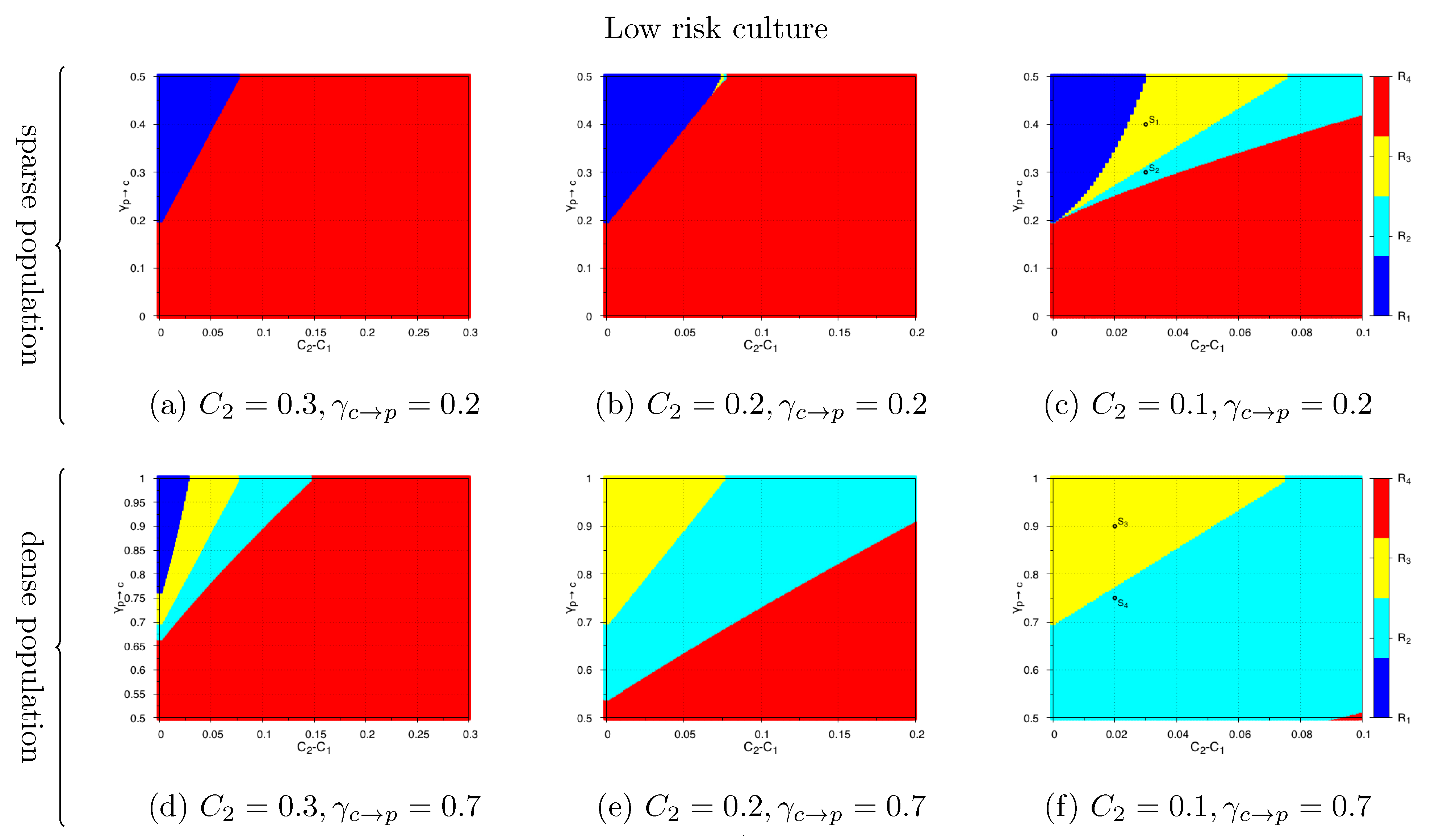
4.1. Low Risk Culture

We consider here the case of a low risk culture scenario as defined previously in Table 1, where the intrinsic transitions toward panic are the most significant ones, and in particular $C_2>C_1$.

It is possible to observe that the number of equilibria of the form $(0,\overline{p},\overline{c},0)$ and the values of $\overline{p}$ and $\overline{c}$ depend only on the parameters $C_1$, $C_2$, ${\gamma }_{p\to c}$ and ${\gamma }_{c\to p}$ (see Appendix B). Here, for each case of Figure 11, we assign different values to the coefficients $C_2$ and ${\gamma }_{c\to p}$, and we investigate the number and the type of equilibria as a function of $C_1$ and ${\gamma }_{p\to c}$. In Figure 11a–c, we consider the case where ${\gamma }_{c\to p}$ and ${\gamma }_{c\to p}$ are less than 0.5, that is, the case of a sparse population. In Figure 11d–f, the imitation coefficients are greater than 0.5, and the scenario of a dense population is taken into account.

Depending on the values of $C_2$ and ${\gamma }_{c\to p}$, we can encounter up to four different behaviors:

• In region $R_1$ (dark blue), we have a unique equilibrium point of the form $(0,\overline{p},\overline{c},0)$, where $\overline{p}<0.5$. Since $\overline{p}+\overline{c}=1$, it means that in this configuration, the density of population with controlled behaviors is greater than $0.5$, and thus, controlled behaviors are predominant during the transient dynamics.
• In region $R_2$ (cyan), there are three equilibrium points of the form $(0,\overline{p},\overline{c},0)$. Two of them exhibit $\overline{p}<0.5,$ while the third one has $\overline{p}>0.5$.
• In region $R_3$ (yellow), there are three equilibrium points of the form $(0,\overline{p},\overline{c},0)$. One of them exhibits $\overline{p}<0.5$, while the other two have $\overline{p}>0.5$.
• In region $R_4$ (red), the system exhibits a unique equilibrium point of the form $(0,\overline{p},\overline{c},0)$, where $\overline{p}>0.5$. For these parameters’ values, our system converges toward an equilibrium with a majority of panic reactions.

It is worth noting that the straight line that separates regions $R_1$ and $R_4$, and regions $R_2$ and $R_3$, has the equation ${\gamma }_{p\to c}-{\gamma }_{c\to p}=4(C_2-C_1)$, and it represents the scenarios when the equilibrium point is $(0,\overline{p},\overline{c},0)=(0,0.5,0.5,0)$, which is the case when the proportion of panic and controlled behaviors have the same value (see Appendix B for supplementary details).

From Figure 11a–d, we note that even in a case of low risk culture, it is possible to have a majority of control behaviors. This is what we have shown in the numerical simulations with the sets of parameters (8) and (10) in regions $R_1$ of Figure 11c,d, respectively. Indeed, in order to have a system that is certain to converge to a configuration with a predominance of controlled behaviors, two properties are needed:

• The difference in value between the intrinsic transitions $C_2$ and $C_1$ must be small.
• The process of imitation from panic to control must dominate the opposite process: that is, the process of imitating individuals in a state of panic. Notably, we were able to demonstrate that the coefficient relating to the imitation from panic to control ${\gamma }_{p\to c}$ must be greater than $4(C_2-C_1)+{\gamma }_{c\to p}$.

These two properties show that in the context of a low risk culture, actions must focus on both intrinsic transitions and imitation processes. This last result could appear counter-intuitive, because it shows that even in a situation where the population is sparse, the imitation process plays a role and must therefore be taken into account by those involved in preventing and managing risks and disasters.

Remark 2.

The choice of parameters $C_1$, $C_2$, ${\gamma }_{p\to c}$ and ${\gamma }_{c\to p}$ we made for the parameter set (7) in Section 3 belong to region $R_4$ in Figure 11a. It is interesting to notice that even if the system we are studying in this section is not exactly the one simulated in Section 3 (for instance, in (7), $B_3$, $B_4$ and the mortality terms are not zero, as we supposed here), the numerical simulations show the same qualitative behavior before $t=70$ min: that is, a predominance of panic reactions (Figure 7). Thus, the qualitative analysis we have developed here can guide the choice of the different parameters.

To complete the information, the values of the parameter set (8) correspond to a point in region $R_1$ of Figure 11a. Finally, the choice of parameters $C_1$, $C_2$, ${\gamma }_{p\to c}$ and ${\gamma }_{c\to p}$ we made for the parameter sets (9) and (10) are in regions $R_4$ and $R_1$ of Figure 11d, respectively.

In regions $R_1$ and $R_4$, the system exhibits a unique equilibrium point, and the system converges to this configuration. Therefore, in these two regions, the system is monostable. On the contrary, in regions $R_2$ and $R_3$, the system is bistable: that is, we have three equilibria, two of them are stable, one with $p<0.5$ and the other with $p>0.5$. As we have stated before, we suppose that the whole population under study at $t=0$ has an everyday behavior: that is, our system starts from the initial condition with $q=1$ and $a=p=c=0.$ We aim to investigate toward which of the two stable equilibria our system will converge. We will show that the parameters involved in the transitions from alert to panic and from alert to control play an important role in the convergence of the system toward a predominance either of panic or control. Further details about the behavior of our system in bistable regions $R_2$ and $R_3$ can be found in Appendix B.

4.2. High Risk Culture

We have repeated the same analysis under the hypothesis of high risk culture: that is, $C_2<C_1$. This time, the theoretical results we found (see Appendix B) lead us to determine $C_1$ and ${\gamma }_{p\to c}$ and to consider the number of equilibria of the form $(0,\overline{p},\overline{c})$ as a function of $C_1-C_2$ and ${\gamma }_{c\to p}$. Here, ${\gamma }_{p\to c}=0.2$ or ${\gamma }_{p\to c}=0.7$ in order to model the two cases of either sparse or dense population. The results are represented in Figure 12. Also in this case, the parameter space is divided into the four regions: $R_1$, $R_2$, $R_3$ and $R_4$.

Figure 12a–d show that even in a configuration with a high risk culture dominated by equilibrium states that converge toward a majority of controlled behaviors, we can still find equilibria around a majority of panic behaviors with certain parameter values. This situation arises when:

• The difference in value between the intrinsic transitions $C_2$ and $C_1$ is small.
• The process of imitation from control to panic is predominant compared to the process in the other direction: that is, the imitation of controlled persons by persons in a state of panic. Notably, we were able to demonstrate that the coefficient relating to the imitation from control to panic ${\gamma }_{c\to p}$ must be greater than $4(C_1-C_2)+{\gamma }_{p\to c}$.

These results show once again that imitation plays an important role and that even in a situation of high risk culture, panic can take over in some scenarios.

The dynamics of the system in bistable regions $R_2$ and $R_3$ can also be analyzed (similarly to the results of Figure A1 in the case of a low risk culture). We observe that in this case, the system mainly converges toward a configuration where the predominant population has a controlled behavior. Moreover, by comparing Figure 11 and Figure 12, it is interesting to note that in a certain sense, regions $R_1$ and $R_4$ are inverted, as are regions $R_2$ and $R_3$.

5. Conclusions

One of the major challenges today for researchers and crisis responders is to understand how a population reacts to a disaster. This paper presents the results of an interdisciplinary collaboration between mathematicians, geographers and psychologists which led to the design of an innovative mathematical model (the APC model) of human behavior in the event of a disaster. Our mathematical modeling approach focused on the macroscopic and collective scale of a population in the event of a sudden disaster without warning signs. We used this approach to study the influence of risk culture and social contagion on behavioral dynamics. We demonstrated in different scenarios (dense or sparse population with different levels of risk culture) how intrinsic transitions and imitation processes have an impact on the development of different panic and controlled behaviors. A calibration of our model has been carried out by exploiting data from a virtual reality experiment in a scenario of a tsunami in Nice (France) [51]. A next step would be to model how the risk of collective panic is managed by the actions and responses of frontline responders [59,60]. In addition, the APC model was not designed to deal with collective pedestrian movements, which can be associated with behaviors in a crisis. It only considers the temporal behavioral dynamics. Spatio-temporal behavioral dynamics will therefore be addressed in future models at different scales. Initial studies have already been developed using diffusion models on networks [35,61]. Finally, a web-based human behavior simulation platform has been developed to provide different audiences (academic experts, operational staff and the general public) with a tool for implementing and using models in a user-friendly interface and for appropriating the behavioral dynamics and envisaged evacuation paths (see www.com2sica.cnrs.fr, Platform tab).

References

1. Dauphiné, A.; Provitolo, D. Risques et Catastrophes: Observer, Spatialiser, Comprendre, Gérer; Armand Colin: Paris, France, 2013. [Google Scholar]
2. Mal, S.; Singh, R.B.; Huggel, C. Climate Change, Extreme Events and Disaster Risk Reduction: Towards Sustainable Development Goals; Springer: Berlin/Heidelberg, Germany, 2017. [Google Scholar]
3. Douvinet, J.; Serra-Llobet, A.; Bopp, E.; Kondolf, G.M. Are sirens effective tools to alert the population in France? Nat. Hazards Earth Syst. Sci. 2021, 21, 2899–2920. [Google Scholar] [CrossRef]
4. Rivera, J.D. Disaster and Emergency Management Methods: Social Science Approaches in Application; Routledge: London, UK, 2021. [Google Scholar]
5. Moussaïd, M. Fouloscopie: Ce Que la Foule Dit de Nous; HumenSciences: Paris, France, 2019. [Google Scholar]
6. Papagiannaki, K.; Kotroni, V.; Lagouvardos, K.; Ruin, I.; Bezes, A. Urban area response to flash flood–triggering rainfall, featuring human behavioral factors: The case of 22 October 2015 in Attica, Greece. Weather Clim. Soc. 2017, 9, 621–638. [Google Scholar] [CrossRef]
7. Ripley, A. The Unthinkable: Who Survives When Disaster Strikes-and Why; Harmony: New York, NY, USA, 2009. [Google Scholar]
8. Ruin, I.; Lutoff, C.; Boudevillain, B.; Creutin, J.D.; Anquetin, S.; Rojo, M.B.; Boissier, L.; Bonnifait, L.; Borga, M.; Colbeau-Justin, L.; et al. Social and hydrological responses to extreme precipitations: An interdisciplinary strategy for postflood investigation. Weather Clim. Soc. 2014, 6, 135–153. [Google Scholar] [CrossRef] [Green Version]
9. Fenet, J.; Daudé, É. La population, grande oubliée des politiques de prévention et de gestion territoriales des risques industriels: Le cas de l’agglomération rouennaise. Cybergeo Eur. J. Geogr. 2020. [Google Scholar] [CrossRef] [Green Version]
10. Crocq, L. Paniques Collectives (Les); Odile Jacob: Paris, France, 2013. [Google Scholar]
11. Quarantelli, E.L. Panic behavior in fire situations: Findings and a model from the English language research literature. In Proceedings of the UJNR Panel on Fire Research and Safety, 4th Joint Panel Meeting, Tokyo, Japan, 13–20 March 1979; pp. 405–428. [Google Scholar]
12. Glass, T.A.; Schoch-Spana, M. Bioterrorism and the people: How to vaccinate a city against panic. Clin. Infect. Dis. 2002, 34, 217–223. [Google Scholar] [CrossRef] [Green Version]
13. Helbing, D.; Mukerji, P. Crowd disasters as systemic failures: Analysis of the Love Parade disaster. EPJ Data Sci. 2012, 1, 7. [Google Scholar] [CrossRef] [Green Version]
14. Dupuy, J.P. La Panique; Les Empêcheurs de Penser en Ronde: Paris, France, 1991. [Google Scholar]
15. Parrochia, D. La Forme des Crises; Éditions du Champ Vallon: Seyssel, France, 2008. [Google Scholar]
16. Keating, J.P. The myth of panic. Fire J. 1982, 76, 57–61. [Google Scholar]
17. Noto, R.; Huguenard, P.; Larcan, A. Médecine de Catastrophe; Masson: Admiralty, France, 1994. [Google Scholar]
18. Drury, J.; Cocking, C.; Reicher, S. Everyone for themselves? A comparative study of crowd solidarity among emergency survivors. Br. J. Soc. Psychol. 2009, 48, 487–506. [Google Scholar] [CrossRef] [Green Version]
19. Mawson, A.R. Understanding mass panic and other collective responses to threat and disaster. Psychiatry Interpers. Biol. Process. 2005, 68, 95–113. [Google Scholar] [CrossRef] [Green Version]
20. Quarantelli, E.L. Conventional beliefs and counterintuitive realities. Soc. Res. Int. Q. 2008, 75, 873–904. [Google Scholar] [CrossRef]
21. Fischer, H.W. Response to Disaster: Fact versus Fiction & Its Perpetuation: The Sociology of Disaster; University Press of America: Lanham, MD, USA, 1998. [Google Scholar]
22. Dubos-Paillard, E.; Connault, A.; Provitolo, D.; Haule, S.; Chalonge, L.; Berred, A. Com2SiCa (2) A database to explore the human behavior at the very moment of disasters. In Proceedings of the AAG 2019 Annual Meeting, Washington, DC, USA, 3–7 April 2019. [Google Scholar]
23. Provitolo, D.; Dubos Paillard, E.; Verdière, N.; Lanza, V.; Charrier, R.; Bertelle, C.; Aziz Alaoui, M. Comportamientos humanos en situación de desastre: De la observación a la modelización conceptual y matemática. Cybergeo Eur. J. Geogr. 2021. [Google Scholar] [CrossRef]
24. Helbing, D.; Molnar, P. Social force model for pedestrian dynamics. Phys. Rev. E 1995, 51, 4282. [Google Scholar] [CrossRef] [PubMed] [Green Version]
25. Zeng, W.; Nakamura, H.; Chen, P. A modified social force model for pedestrian behavior simulation at signalized crosswalks. Procedia-Soc. Behav. Sci. 2014, 138, 521–530. [Google Scholar] [CrossRef] [Green Version]
26. Cornes, F.; Frank, G.; Dorso, C.O. Fear propagation and the evacuation dynamics. Simul. Model. Pract. Theory 2019, 95, 112–133. [Google Scholar] [CrossRef]
27. Tong, W.; Cheng, L. Simulation of pedestrian flow based on multi-agent. Procedia-Soc. Behav. Sci. 2013, 96, 17–24. [Google Scholar] [CrossRef] [Green Version]
28. Martinez-Gil, F.; Lozano, M.; García-Fernández, I.; Fernández, F. Modeling, evaluation, and scale on artificial pedestrians: A literature review. ACM Comput. Surv. CSUR 2017, 50, 1–35. [Google Scholar] [CrossRef] [Green Version]
29. Chalons, C.; Goatin, P.; Seguin, N. General constrained conservation laws. Application to pedestrian flow modeling. Netw. Heterog. Media 2013, 8, 433. [Google Scholar] [CrossRef]
30. Bellomo, N.; Dogbe, C. On the modeling of traffic and crowds: A survey of models, speculations, and perspectives. SIAM Rev. 2011, 53, 409–463. [Google Scholar] [CrossRef]
31. Sanders, L. Models in Spatial Analysis; John Wiley & Sons: Hoboken, NJ, USA, 2013. [Google Scholar]
32. Maury, B.; Faure, S. Crowds in Equations: An Introduction to the Microscopic Modeling of Crowds; World Scientific: Singapore, 2018. [Google Scholar]
33. Banos, A.; Lang, C.; Marilleau, N. Agent-Based Spatial Simulation with NetLogo, Volume 2: Advanced Concepts; Elsevier: Amsterdam, The Netherlands, 2016. [Google Scholar]
34. Daudé, E.; Chapuis, K.; Taillandier, P.; Tranouez, P.; Caron, C.; Drogoul, A.; Gaudou, B.; Rey-Coyrehourcq, S.; Saval, A.; Zucker, J.D. ESCAPE: Exploring by simulation cities awareness on population evacuation. In Proceedings of the 16th International Conference on Information Systems for Crisis Response and Management (ISCRAM 2019), Valencia, Spain, 19–22 May 2019; pp. 76–93. [Google Scholar]
35. Lanza, V.; Dubos-Paillard, E.; Charrier, R.; Verdière, N.; Provitolo, D.; Navarro, O.; Bertelle, C.; Cantin, G.; Berred, A.; Aziz-Alaoui, M. Spatio-Temporal Dynamics of Human Behaviors During Disasters: A Mathematical and Geographical Approach. In Complex Systems, Smart Territories and Mobility; Springer: Berlin/Heidelberg, Germany, 2021; pp. 201–218. [Google Scholar]
36. Massaguer, D.; Balasubramanian, V.; Mehrotra, S.; Venkatasubramanian, N. Multi-agent simulation of disaster response. In Proceedings of the ATDM Workshop in AAMAS, Hakodate, Japan, 8–12 May 2006; Volume 2006. [Google Scholar]
37. D’Orazio, M.; Spalazzi, L.; Quagliarini, E.; Bernardini, G. Agent-based model for earthquake pedestrians’ evacuation in urban outdoor scenarios: Behavioural patterns definition and evacuation paths choice. Saf. Sci. 2014, 62, 450–465. [Google Scholar] [CrossRef]
38. Wang, X.; Zhang, L.; Lin, Y.; Zhao, Y.; Hu, X. Computational models and optimal control strategies for emotion contagion in the human population in emergencies. Knowl.-Based Syst. 2016, 109, 35–47. [Google Scholar] [CrossRef]
39. Cantin, G.; Verdière, N.; Lanza, V.; Aziz-Alaoui, M.; Charrier, R.; Bertelle, C.; Provitolo, D.; Dubos-Paillard, E. Mathematical modeling of human behaviors during catastrophic events: Stability and bifurcations. Int. J. Bifurc. Chaos 2016, 26, 1630025. [Google Scholar] [CrossRef]
40. Festinger, L. A theory of social comparison processes. Hum. Relat. 1954, 7, 117–140. [Google Scholar] [CrossRef]
41. Fiske, S.T.; Taylor, S.E. Social Cognition: From Brains to Culture; Sage: Newcastle upon Tyne, UK, 2013. [Google Scholar]
42. Mikolajczak, M.; Desseilles, M. Traité de Régulation des Émotions; De Boeck Supérieur: Bruxelles, Belgium, 2012. [Google Scholar]
43. Provitolo, D.; Tricot, A.; Schleyer-Lindenmann, A.; Boudoukha, A.; Verdière, N.; Haule, S.; Dubos-Paillard, E.; Lanza, V.; Charrier, R.; Bertelle, C.; et al. Saisir les comportements humains en situation de catastrophes: Proposition d’une démarche méthodologique immersive. Cybergeo Rev. Eur. Géogr./Eur. J. Geogr. 2022. [Google Scholar] [CrossRef]
44. Moussaïd, M.; Kapadia, M.; Thrash, T.; Sumner, R.W.; Gross, M.; Helbing, D.; Hölscher, C. Crowd behaviour during high-stress evacuations in an immersive virtual environment. J. R. Soc. Interface 2016, 13, 20160414. [Google Scholar] [CrossRef] [PubMed] [Green Version]
45. Verhulst, E.; Richard, P.; Provitolo, D.; Navarro-Carrascal, O. Virtual Tsunami: Navigation technique and user behavior analysis during emergency. In Proceedings of the 1st International Conference for Multi-Area Simulation-ICMASim, Angers, France, 8–10 October 2019. [Google Scholar]
46. Boschetti, L.; Provitolo, D.; Tric, E. A method to analyze territory resilience to natural hazards, the example of the French Riviera against tsunami. In Proceedings of the EGU General Assembly Conference Abstracts, Vienna, Austria, 23–28 April 2017; Volume 19, p. 12935. [Google Scholar]
47. Russell, J.A. A circumplex model of affect. J. Personal. Soc. Psychol. 1980, 39, 1161. [Google Scholar] [CrossRef]
48. Bandura, A. Social Learning Theory; General Learning Press: Morristown, NJ, USA, 1971. [Google Scholar]
49. Laborit, H. La légende des Comportements; Flammarion: Paris, France, 1994. [Google Scholar]
50. Selye, H. The stress concept. Can. Med. Assoc. J. 1976, 115, 718. [Google Scholar]
51. Verdière, N.; Navarro, O.; Naud, A.; Berred, A.; Provitolo, D. Towards Parameter Identification of a Behavioral Model from a Virtual Reality Experiment. Mathematics 2021, 9, 3175. [Google Scholar] [CrossRef]
52. Hethcote, H.W. The mathematics of infectious diseases. SIAM Rev. 2000, 42, 599–653. [Google Scholar] [CrossRef] [Green Version]
53. Brauer, F. Compartmental Models in Epidemiology. In Mathematical Epidemiology; Brauer, F., van den Driessche, P., Wu, J., Eds.; Lecture Notes in Mathematics; Springer: Berlin/Heidelberg, Germany, 2008; Volume 1945. [Google Scholar] [CrossRef]
54. Jacquez, J.A.; Simon, C.P. Qualitative theory of compartmental systems. SIAM Rev. 1993, 35, 43–79. [Google Scholar] [CrossRef]
55. Gilbert, D.T.; Giesler, R.B.; Morris, K.A. When comparisons arise. J. Personal. Soc. Psychol. 1995, 69, 227. [Google Scholar] [CrossRef]
56. Martin, A.; Guéguen, N.; Fischer-Lokou, J. L’imitation humaine: Une synthèse de 50 années de recherche en psychologie sociale. Can. Psychol. Can. 2016, 57, 101. [Google Scholar] [CrossRef] [Green Version]
57. Baudonnière, P.M. Le Mimétisme et L’imitation; Flammarion, Dominos: Paris, France, 1997. [Google Scholar]
58. Ghesquiere, F.; Kellett, J.; Campbell, J.; Kc, S.; Reid, R. The Sendai Report: Managing Disaster Risks for a Resilient Future; Technical Report; The World Bank: Washington, DC, USA, 2012. [Google Scholar]
59. Verdière, N.; Dubos-Paillard, E.; Lanza, V.; Provitolo, D.; Charrier, R.; Bertelle, C.; Berred, A.; Tricot, A.; Aziz-Alaoui, M. Study of the Effect of Rescuers and the Use of a Massive Alarm in a Population in a Disaster Situation. Sustainability 2023, 15, 9474. [Google Scholar] [CrossRef]
60. Mikiela, I.; Lanza, V.; Verdière, N.; Provitolo, D. Optimal strategies to control human behaviors during a catastrophic event. AIMS Math. 2022, 7, 18450–18466. [Google Scholar] [CrossRef]
61. Lanza, V.; Dubos-Paillard, E.; Charrier, R.; Provitolo, D.; Berred, A. An analysis of the effects of territory properties on population behaviors and evacuation management during disasters using coupled dynamical systems. Appl. Netw. Sci. 2022, 7, 17. [Google Scholar] [CrossRef]
62. Alesina, A.; Galuzzi, M. Vincent’s Theorem from a modern point of view. Rend. Circ. Mat. Palermo 2000, 64, 179–191. [Google Scholar]
63. Akritas, A.; Strzeboński, A.; Vigklas, P. On the various bisection methods derived from Vincent’s theorem. Serdica J. Comput. 2008, 2, 89–104. [Google Scholar] [CrossRef]
Figure 1. Analysis and comparison of the two behavioral modeling approaches based either on individual descriptions leading to multi-agent systems or on descriptions of populations leading to dynamical systems (top of the figure). The agent-based approach requires an element of randomness when generating individuals because knowledge or data serving as a reference is only available at the scale of populations.
Sustainability 15 11063 g001
Figure 2. Diagram of how national and local policymakers can take action and analyze the simulations depending on the choice of model. The individual/agent approach requires measures at the population scale to study the impact of possible actions.
Sustainability 15 11063 g002
Figure 3. The classification of the different behaviors during a catastrophic event organized according to the emotional charge and its regulation.
Sustainability 15 11063 g003
Figure 4. Transfer diagram for the APC (Alert, Panic and Control) model. The intrinsic transitions are represented in solid lines, while the imitation ones are in dashed lines.
Sustainability 15 11063 g004
Figure 5. Function ξ in the imitation interactions terms. This sygmoidal function was chosen to model the fact that the behavior of the majority is the most imitated behavior.
Sustainability 15 11063 g005
Figure 6. Functions (a) γ ( t ) = ζ ( t , 1 , 3 ) and (b) φ ( t ) = ζ ( t , 70 , 100 ) . Function γ increases sharply from τ 0 = 1 and τ 1 = 3 to model the fact that after three minutes, the majority of the population with an everyday behavior becomes alert. We suppose that people can only return to everyday life behavior after 70 min from the beginning of the catastrophe; therefore, we choose τ 0 = 70 for function φ .
Sustainability 15 11063 g006
Figure 7. Two examples of a dense population with a low risk culture for the set of parameters (7) (in (ac)) and (8) (in (df)). For both cases, (a,d) on the left represent the flux toward control due to intrinsic (green solid line) or imitation (blue dashed line) transitions. In the center, (b,e) compare the flux toward panic due to intrinsic (green solid line) or imitation (blue dashed line) transitions. Finally, on the right, (c,f) represent the time evolution of the three main populations a, p and c.
Sustainability 15 11063 g007
Figure 8. Two examples of a sparse population with a low risk culture for the set of parameters (9) (in (ac)) and (10) (in (df)). For both cases, (a,d) on the left represent the flux toward control due to intrinsic (green solid line) or imitation (blue dashed line) transitions. In the center, (b,e) compare the flux toward panic due to intrinsic (green solid line) or imitation (blue dashed line) transitions. Finally, on the right, (c,f) represent the time evolution of the three main populations a, p and c.
Sustainability 15 11063 g008
Figure 9. Example of a dense population with a high risk culture. (a) Flux toward control due to intrinsic (green solid line) or imitation (blue dashed line) transitions. (b) Flux toward panic due to intrinsic (green solid line) or imitation (blue dashed line) transitions. (c) Time evolution of the three main populations a, p and c. Here, I m c is greater than I n c ; thus, the imitation transitions toward control are the predominant ones and almost 90% of the population adopts a controlled behavior (see (c)).
Sustainability 15 11063 g009
Figure 10. Example of a sparse population with a high risk culture. (a) Flux toward control due to intrinsic (green solid line) or imitation (blue dashed line) transitions. (b) Flux toward panic due to intrinsic (green solid line) or imitation (blue dashed line) transitions. (c) Time evolution of the three main populations a, p and c. Here, I n c is greater than I m c ; thus, the intrinsic transitions toward control are the predominant ones, and after a transient phase, control is the most adopted behavior.
Sustainability 15 11063 g010
Figure 11. Equilibria of the form ( 0 , p ¯ , c ¯ , 0 ) in the hypothesis of low risk culture, as a function of C 2 C 1 and γ p c . In (ac), a sparse population is considered, while in (df), a dense population is taken into account. The parameter space is divided into four regions: R 1 is the mono-stability region with predominance of control; in region R 2 , we have three equilibria with two of them with p ¯ < 0.5 ; in region R 3 , we have three equilibria with two of them with p ¯ > 0.5 ; finally, R 4 is the mono-stability region with a predominance of panic. The system behavior in the points labeled as S 1 and S 2 in (c), and S 3 and S 4 in (f), is analyzed in greater detail in Figure A1.
Sustainability 15 11063 g011
Figure 12. Equilibria of the form ( 0 , p ¯ , c ¯ , 0 ) in the hypothesis of a high risk culture as a function of C 1 C 2 and γ c p . In (ac), a sparse population is considered, while in (df), a dense population is taken into account. The parameter space is divided into four regions: R 1 is the mono-stability region with a predominance of control; in region R 2 , we have three equilibria with two of them with p ¯ < 0.5 ; in region R 3 , we have three equilibria with two of them with p ¯ > 0.5 ; finally, R 4 is the mono-stability region with a predominance of panic.
Sustainability 15 11063 g012