Article

Application of Improved Particle Swarm Optimization SVM in Water Quality Evaluation of Ming Cui Lake

1
School of Civil Engineering, North Minzu University, Yinchuan 750021, China
2
Department of Architecture, Lyuliang University, Lvliang 033000, China
3
School of Electrical & Information Engineering, North Minzu University, Yinchuan 750021, China
4
Shandong Saibao Electronic Information Products Supervision and Testing Institute, Jinan 250013, China
*
Author to whom correspondence should be addressed.
Sustainability 2023, 15(12), 9835; https://doi.org/10.3390/su15129835
Submission received: 6 May 2023 / Revised: 31 May 2023 / Accepted: 15 June 2023 / Published: 20 June 2023
(This article belongs to the Special Issue Sustainability in Water Treatment)

Abstract

:
Water quality directly determines our living environment. In order to establish a more scientific and reasonable water quality evaluation model, it needs a lot of data support, but it will lead to a large increase in the calculation time of the evaluation model. This paper proposes an improved particle swarm optimization SVM model (CPOS-SVM) to solve this problem. In this paper, the Pareto optimal solution concept is used to sparsely process the training set, which can ensure that the number of training sets is reduced without loss of data characteristics, thus reducing the training time. In order to solve the problem of the kernel parameter g and penalty factor c on the SVM algorithm, which affects the accuracy of the SVM model but it is difficult to select why, a particle swarm optimization algorithm is used in this paper to optimize the kernel parameter and penalty factor and improve the accuracy of the model. In this paper, 480 sets of data from Ming Cui Lake from 2014 to 2022 are taken as the research object, and examples are analyzed in MATLAB 2020a. The results show that the training time of the CPOS-SVM model can be completed within 2 s and does not increase with the increase of data volume. Meanwhile, by comparing the SVM model, POS-SVM model, and POS-BP model, training time increases dramatically with the amount of data. The accuracy of the POS-SVM model is the highest, and the accuracy of the CPOS-SVM model is basically consistent with that of the POS-SVM, reaching 94%, while the accuracy of the SVM model and the POS-BP model are slightly worse. This indicates that the CPOS-SVM model has good application value in water quality evaluation.

1. Introduction

With the arrival of a new era, China’s society and economy have made significant progress, but the impact on the environment has also grown. The government’s emphasis on “green mountains and clear waters” has made water quality management a top priority. Studies show that surface water is highly susceptible to adverse sources of pollution, and the water environment system is facing many urgent problems [1]. Accurate water quality assessments offer scientific guidance for managing, protecting, and governing water environments, as well as guiding wastewater treatment planning goals and directions [2].
Water quality is affected by various factors such as organic pollutants, harmful by-products, pathogenic microorganisms, iron, manganese substances, and ammonia nitrogen pollutants. To determine the water quality grade, parameters such as ammonia nitrogen content, dissolved oxygen, permanganate content, total phosphorus, and total nitrogen are usually measured [2]. Currently, water quality assessment methods using physical and chemical factors can be divided into a single-factor evaluation and a multi-factor comprehensive evaluation. The single-factor evaluation method is simple to use and has low uncertainty. However, it is too narrow to fully evaluate water quality [2,3,4,5]. Dimensionless processing techniques, such as maximum value, mean value, and normalization, are used to process data. However, these methods are susceptible to the influence of extreme values and are not suitable for areas with poor water quality. Some researchers use multi-factor comprehensive evaluation methods such as grey relational degree analysis [6], artificial neural network [7,8], and support vector machine [9,10].
Scholars have improved traditional methods by standardizing the processing of raw data in a dimensionless way, making them less susceptible to the influence of extreme values. They have also rewritten the absolute difference formula to increase the calculation accuracy by using a point-to-interval form. However, these methods are subjective and cannot effectively solve the one-sidedness of the evaluation. Esakkimuthu Tharmar used principal component analysis (PCA) to find out the dominant factors of the overall water quality and its variance coverage [11]. Neural networks excel in solving nonlinear problems and can approximate nonlinear functions with sufficient training data. The backpropagation (BP) neural network is one of the most basic and widely used in neural networks today [10]. Applying the BP neural network to water quality evaluations, we analyzed the main factors affecting water quality changes. Compared with the comprehensive index evaluation method, the BP neural network evaluation process is more convenient and the evaluation results are more objective. However, the BP neural network is limited by the convergence speed and may fall into local minimum values. Additionally, when the sample data is small, the error is larger [3,7,12,13]. Yang Cheng et al. partly solved the problem of traditional methods easily falling into local minimums and enhanced system robustness by using the T-S fuzzy neural network model [14]. However, the convergence speed and prediction accuracy are still insufficient. Chen Yaoning et al. evaluated and predicted the water quality of Baiyun Lake using the support vector machine method, which has good generalization and extrapolation capabilities and can solve the water quality evaluation accuracy problem well [15]. However, it is greatly restricted in convergence speed when facing large-scale data training, and the selection of kernel parameters and penalty factors seriously affects the classification accuracy of the support vector machines. Ref. [16] proposed to use machine learning to predict groundwater quality. Different machine learning methods had good results for different parameters, but no machine learning algorithm had good results for all parameters. Rongli Gai and Zhibin Guo [17] proposed an improved grey relational degree method and particle swarm optimization multi-classification SVM algorithm to evaluate river water quality. Hítalo Tobias Lôbo Lopes used a nonlinear model to predict data, but the accuracy rate was not high [18]. Firstly, the correlation indexes of factors affecting the water quality were extracted, and the four indexes with the greatest correlation were found as the input of the particle swarm optimization multi-classification SVM algorithm to evaluate the quality of the river water environment. Although this algorithm can ignore the influencing factors with little correlation, it also ignores the essential characteristics of some original data in this process, which may cause deviations in specific working conditions.
In view of the limitations of the methods proposed in the above papers, this paper improved the model training speed and prediction accuracy. The innovation points are summarized as follows: 1. Aiming at the problem of geometric increase of training time caused by an excessive training set of the SVM model, the concept of Pareto optimal solution is put forward to sparse training set data, which can improve the training speed without affecting the prediction accuracy. 2. The selection of kernel parameters and penalty factors of SVM will affect the classification accuracy of the support vector machine. To solve the problem of the difficult selection of hyperparameters, a particle swarm optimization algorithm is used in this paper to select the hyperparameters and improve the accuracy of the model. By accurately assessing the water quality classification, the degree and source of water pollution can be accurately assessed, the sources of water pollution can be discovered and eliminated in time, and the water resources and ecological environment can be effectively protected, thus promoting environmental protection. At the same time, an accurate water quality assessment method can improve the utilization efficiency of water resources, ensure the supply quality of water resources, and improve the green technology and cost-effectiveness of environmental governance, so as to achieve sustainable development.

2. Materials and Methods

2.1. Data Collection

All water quality test data were taken from the water quality data of the Ming Cui Wetland Park, Yinchuan, Ningxia from 2014 to 2021. Ming Cui Lake is located in Zhangzheng Town, east of the Xingqing District, Yinchuan City, covering an area of more than 10,000 mu and an average water depth of 2.12 m. It mainly relies on the Yellow River irrigation and farmland water replenishment. In 2005, it was listed as a wetland park by the People’s Government of Ningxia Hui Autonomous Region, and in 2006, it was identified as a National Wetland Park by the State Forestry Administration. In recent years, due to excessive exploitation and utilization, and the decline of biological resources in Ming Cui Lake water, some waters show a trend of ecological desertification, serious aquatic ecosystem damage, and the inevitable exogenous pollution of farmland water retreat, leading to the aggravation of lake eutrophication and the function of the aquatic ecosystem in the lake area [14]. Therefore, this paper proposes a comprehensive evaluation of the water quality of Ming Cui Lake based on the improved particle swarm optimization SVM algorithm, which can provide accurate results in the comprehensive prevention and control of Ming Cui Lake water pollution.
This article uses the water quality monitoring data from the Ming Cui Lake Wetland Park in Yinchuan, Ningxia Hui Autonomous Region from 2014 to 2021 as the research object. A water quality evaluation is used to determine the water quality level by combining various indicators of sampled water quality and various water quality standards using mathematical models. The water quality indicators used in this study include ammonia nitrogen, dissolved oxygen, permanganate index, total phosphorus, and total nitrogen, with the corresponding grade standards shown in Table 1.

2.2. Proposed Methods

2.2.1. SVM Models

The SVM algorithm was initially designed to solve linearly separable problems. Taking two dimensions as an example, for a given sample set x 1 and y 1 :
D = { ( x 1 , y 1 ) , ( x 2 , y 2 ) }     x R n , y { 1 , 1 }
As shown in Figure 1, the hollow and solid points belong to different categories, and the purpose is to find a hyperplane that can divide these two categories of points with the maximum margin. In order to minimize the influence of local disturbances on the results and make the classification results robust and generalizable, the margin of the hyperplane should be maximized. The dividing hyperplane can be defined as a linear equation:
w T X + b = 0
where w = { w 1 ; w 2 ; ; w d } is the normal vector that determines the direction of the hyperplane, d is the number of features, X is the training sample, and b is the displacement. As long as the normal vector (w) and displacement (b) are determined, a hyperplane can be uniquely determined. In this way, the points on both sides of the hyperplane can be represented as either w T X + b > 0 or w T X + b < 0 , and adjusting w defines two hyperplanes as w T X + b = 1 and w T X + b = 1 .
Thus, all points located above the plane with a value less than 0 are classified as type −1, and all points located below the plane with a value greater than 0 are classified as type 1. The distance between any point on the dividing hyperplane and the two margin hyperplanes on both sides is 1 w , and to maximize this distance, the problem can be transformed into a convex optimization problem with an optimization model y i * ( w 0 + w 1 x 1 + w 2 x 2 ) 1 and limited parameters i .
M A X i M i z e w ( a ) = i = 1 N a i 1 2 i , j = 1 N a i a j y i y j x i x j
i = 1 N a i y i = 0 a 0 , i = 1 , 2 , , N
After the optimal a i is obtained using Lagrange’s formula and the KTT conditional optimization formula, those a i that are not equal to 0 are the support vectors we need, w 0 can be solved under the constraint of 0, and the classification function obtained is as follows:
f ( x ) = sgn ( ( w * ) T x + w 0 ) = sgn ( i = 1 N a * y i x i * + w 0 * )
In many cases, the original data itself may not be separable, in which case, a soft margin can be introduced by introducing a variable ξ i to relax the constraints as follows:
y i ( w i · x + b ) 1 1 ξ i
which introduces a penalty parameter C to the objective function:
ϕ ( w , ξ ) = 1 2 w 2 + C i = 1 N ξ i
When the original data cannot be classified using a hyperplane, an appropriate kernel function can be introduced to handle the original data by mapping it from a low-dimensional feature space to a high-dimensional one. This approach solves the relatively complex computational problem in the low-dimensional space and converts the original non-separable data into a linearly separable one. The original data features (x) are transformed into a nonlinear form ( Z = φ ( x ) ), which corresponds to a quadratic optimization problem that can be expressed as follows:
M A X i M i z e w ( a ) = i = 1 N a i 1 2 i , j = 1 N a i a j y i y j ( φ ( x i ) · φ ( x i ) )
i = 1 N a i y i = 0     a 0 , i = 1 , 2 , , N
We used the support vector to solve b:
y i ( i = 1 N a i y i ( K ( x i , x j ) + b ) ) 1 = 0
It can be concluded from the above that the kernel parameter K can affect the classification accuracy of the model, while the penalty factor (C) affects the generalization and regularization of the model. If C is set to a very high value, it can cause overfitting of the SVM model.

2.2.2. The Pareto Optimal Solution Principle

The SVM algorithm is particularly suitable for training with small sample sizes. However, when a large number of samples are used to train an SVM model, there may be issues related to computational efficiency. On the other hand, small capacity sample data is not sufficient to characterize classification characteristics. Therefore, it is important to address the issue of the sparsification of data without reducing the support vectors and maintaining data characteristics.
Pareto solutions, also known as non-dominated solutions, arise when dealing with multiple objectives. Due to the existence of conflicts or incomparable objectives, a single solution can be the best in one objective but the worst in others. Changing any objective will inevitably weaken at least one other objective’s solution, thus creating non-dominated solutions or Pareto solutions. A set of optimal solutions of an objective function is called Pareto optimal set. The mathematical model is as follows:
{ min y = F ( x ) = ( f 1 ( x ) , f 2   ( x ) , , f m   ( x ) ) T g i ( x )               0 , i = 1 , 2 , , p   h j ( x )               0 , j = 1 , 2 ,   , q  
In the equation, x = [ x 1 , x 2 , , x n ] X R n is an n-dimensional decision variable vector, X is an n-dimensional decision space, y = [ y 1 , y 2 , , y n ] Y R M is an M-dimensional objective function vector, and Y is an M-dimensional objective space. The M objective functions, defined in F(x), create M mapping functions that map the decision space to the objective space. g i ( x ) 0 ( i = 1 , 2 , , p ) defines the p inequality constraints, and h i ( x ) 0 ( i = 1 , 2 , , q ) defines the q inequality constraints. Here are several related definitions:
(1) Dominance: if there exists i [ 1 , m ] , f i ( x ) f i ( x ) and j [ 1 , m ] , f i ( x ) < f i ( x ) such that x dominates x .
(2) Non-dominance: if there does not exist x that satisfies the above conditions, then x is a non-dominated solution to x .
(3) Pareto optimal solution: if there is no point x that dominates x in the entire search space, then x is a Pareto optimal solution.
(4) Pareto optimal set: the set of Pareto optimal solutions.

2.2.3. Particle Swarm Optimization Algorithm

Particle swarm optimization (PSO) is an intelligent algorithm that seeks approximate optimal solutions with high accuracy and simple implementation. Compared to other evolutionary algorithms, PSO retains global search capability. Its search strategy is a velocity displacement model, avoiding relatively complex genetic operations. Furthermore, due to its memory of each particle, the PSO algorithm can dynamically adjust the search strategy during the entire operation process. The specific process diagram is shown in Figure 2.
The updated strategy for particle position and velocity is shown below:
v i d k + 1 = w v i d k + c 1 × r a n d 1 k × ( P b e s t i d k x i d k ) + c 2 × r a n d 2 k × ( G b e s t d k x i d k )
x i d k + 1 = x i d k + v i d k + 1
In the above two formulas, w is the inertia weight factor, c 1 and c 2 are non-negative acceleration constants, r a n d 1 and r a n d 2 are uniformly distributed random numbers between 0 and 1, P b e s t i d ( k ) represents the individual optimal solution at iteration k, and G b e s t i d ( k ) represents the global optimal solution at iteration k.

2.2.4. CPSO-SVM

Generally, loop validation is used for SVM parameter optimization. The basic idea is to divide the original data into groups, with one part as the testing set and the other part as the validation set. Then, all combinations of parameters g and c in the value space are verified to find the best parameter combination. In this method, the classifier is first trained with the training set, and then the trained model is tested with the validation set to obtain the classification accuracy as the performance evaluation index of the classifier. However, this method has a high time complexity and requires a lot of computing time. In this paper, the particle swarm optimization (PSO) algorithm is used to find the optimal parameters of g and c. By continuously updating the particle position and velocity, the optimization is realized, and evolutionary iteration is constantly performed to quickly calculate the optimal g and c. The CPSO-SVM algorithm process is shown in Figure 3.

2.2.5. Data Preprocessing

In this article, Pareto optimality is used to sparsify the original data in order to reduce the number of training samples and speed up the training process. To maintain the original characteristics of the training samples, the support vectors of a support vector machine are observed to be located at the edges of the data set when solving for the hyperplane. Therefore, the Pareto optimal solution set and the corresponding worst solution set for the water quality level are obtained. As shown in Figure 4, the non-dominated solutions, composed of A1, A2, A3, etc., represent the optimal solutions, while the dominated solutions, composed of B1, B2, B3, etc., are not dominated by other solutions and are closest to the next water quality level. The intermediate solution set, such as C1, C2, C3, etc., can be directly removed.
In general, methods such as centralization, maximum-minimum normalization, averaging, or range normalization are commonly used for the dimensionless processing of raw data. However, since the standard range of water quality is uneven, these methods may change the discretization of sequential data. This article proposes a new normalization method, the correlation coefficient calculation method based on linear operations, which can make the numerical differences between different water quality levels more obvious. The formula for this method is as follows:
y i = x i x i min x i max x i min ( y i max y i min ) + y i min
In the formula, x i represents the raw data, x i min represents the minimum value of the raw data in the corresponding water quality level, x i max represents the maximum value of the data in the corresponding water quality level, y i represents the processed data, y i max represents the maximum value of the processed data in the corresponding water quality level, and y i min represents the minimum value of the processed data in the corresponding water quality level.

3. Results

To verify the effectiveness and reliability of the CPOS-SVM model in water quality prediction, this study used the water quality monitoring data from the Ming Cui Wetland Park in Yinchuan, Ningxia Hui Autonomous Region, from 2014 to 2021 as the research object. To ensure the cognitive and generalization abilities of the trained network, while taking into account both the commonality and individuality of the samples, the study used the different methods between adjacent water quality standards of two categories in the national “Surface Water Environmental Quality Standard” to obtain sample data. A total of 620, 1020, 1520, and 2020 sets of sample data were generated, including 140, 540, 1040, and 1540 sets of data, respectively. The sample data were randomly divided into a test set and a training set. Among them, 50 sets of monitoring data and 100 sets of randomly selected generated sample data were used as a test set to detect the accuracy of the trained model, and the remaining data were used as a training set to train the model.The specific data division is shown in Table 2. In order to demonstrate the superiority of the proposed algorithm, CPOS-SVM, POS-SVM, POS-BP, and SVM were compared with different model parameter settings. The parameter Settings of the above four algorithms shown in “Algorithm 1, Algorithm 2, Algorithm 3 and Algorithm 4”.
Table 2. Training model data partitioning.
Number of Data SetsNumber of Training SetsNumber of Test Set Groups
620 groups470150
1020 groups870150
1520 groups1370150
2020 groups1870150
Algorithm 1: Using Pareto solutions to sparsify the sample data as the training samples, with a population size of N = 10, a maximum iteration number of T = 200, learning factors c 1 = c 2 = 2, a search range of [−6,6], and control parameters k1 = k2.
Algorithm 2: Without sparsifying the sample data, with a population size of N = 10, a maximum iteration number of T = 200, learning factors c 1 = c 2 = 2, a search range of [−6,6], and control parameters k1 = k2.
Algorithm 3: With a population size of N = 10, a maximum iteration number of T = 200, learning factors c 1   = c 2 = 2, a search range of [−6,6], control parameters k1 = k2, an input layer node of 5, a hidden layer node of 10, an output layer node of 1, and a maximum training number of 1000 for BP neural network. The transfer functions for the hidden layer and output layer are logsig and purelin, the training function is trainlm, the learning rate is 0.01, and the training error target is 0.001.
Algorithm 4: Directly assigning c = 0.5 and g = 3.48 obtained from Algorithm 1 via particle swarm optimization as the penalization factor and kernel function interval for the SVM algorithm.
The different algorithms were run five times, and the average of the running time and the results on the water quality prediction test set were taken as the final results, as shown in Figure 5 and Figure 6. Meanwhile, the comparison between the predicted data and the real data of the best test set results of the four algorithms on the 1020 data sets were given in Figure 7, Figure 8, Figure 9 and Figure 10.
The computational time varies greatly among the models, with SVM being the fastest due to its parameters being directly given and not requiring the POS algorithm to search. The second fastest is the CPOS-SVM algorithm, which requires data preprocessing when the data set is relatively small. Since there are not many redundant data to be removed, its advantage is not obvious. However, when the data set increases, after data preprocessing and removing excess data, the sample data size is reduced, which only slightly increases the running time. On the other hand, the running time of the other algorithms is relatively long due to the increase in data volume.
In terms of accuracy, the CPOS-SVM model and the POS-SVM model have almost the same accuracy as SVM, which suggests that sparsifying the training set with Pareto optimal solutions does not lead to a loss of the original data features and can fully preserve the characteristics of the data. As the original data increases, the accuracy of the models increases significantly, especially for the POS-BP model. The accuracy of the CPOS-SVM model is better than that of the POS-BP model on both the training set and the test set, which indicates that the CPOS-SVM model has stronger stability and robustness in the water quality evaluation.
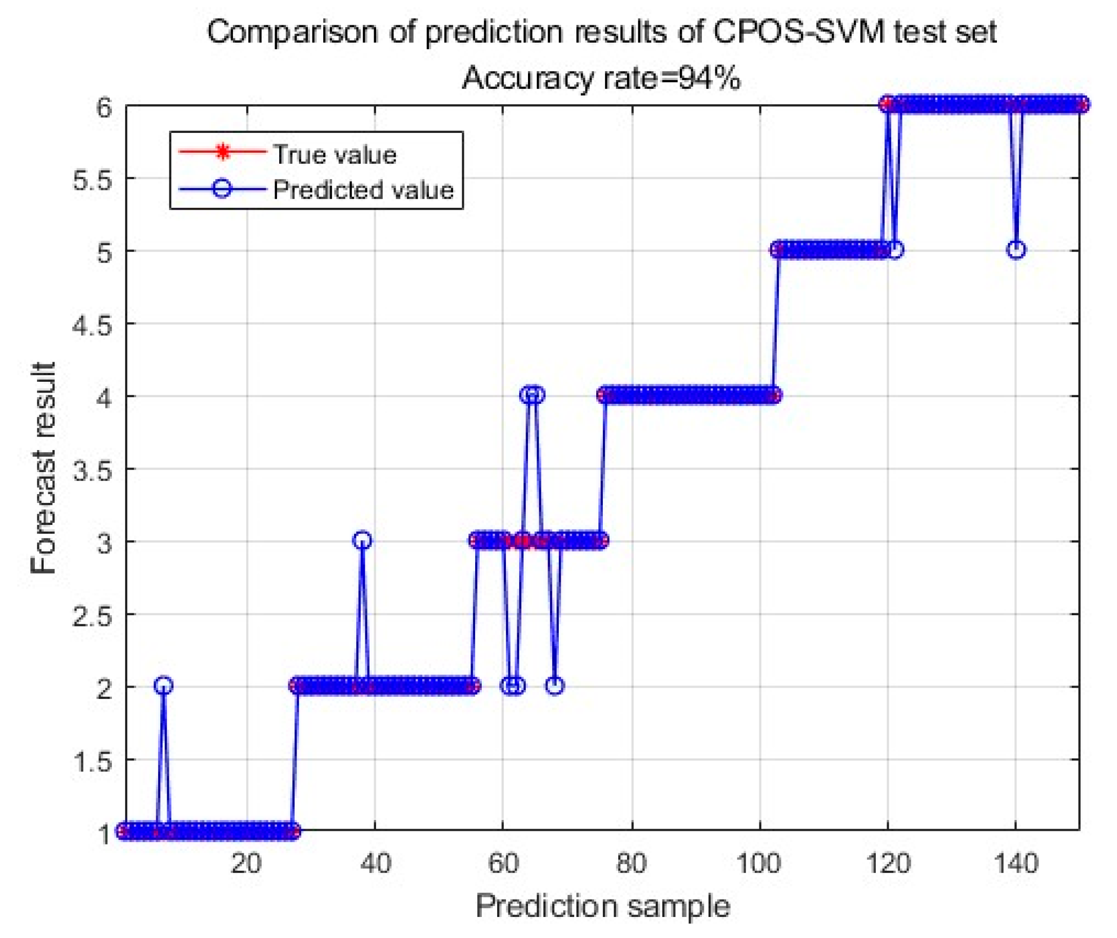
Figure 7, Figure 8, Figure 9 and Figure 10 respectively show the specific classification results of the CPOS-SVM, POS-SVM, POS-BP, and SVM algorithms. It can be seen from the figures that the SVM algorithm has the highest accuracy, which is because the SVM algorithm has not undergone data sparsity processing and retains all features of the original data. However, it can be seen from Figure 5 that its training time is greatly increased. The accuracy of the CPOS-SVM algorithm is slightly affected, but the training speed is greatly improved. This is because the characteristics of the original data are not affected when the CPOS-SVM algorithm is sparse, while the POS-SVM and POS-BP algorithms have advantages in both accuracy and training speed.

4. Conclusions

In this paper, the concept of Pareto optimal solution is used to sparsely process the training data, which greatly improves the operation speed while preserving the characteristics of the original data. To solve the problem of the difficult selection of the kernel parameters and the penalty coefficient of the SVM algorithm, particle swarm optimization was proposed to improve the accuracy of the model. Taking the water quality test data of Ming Cui Lake from 2014 to 2021 as the research object, model parameters of different algorithms were set, and the POS-SVM model, POS-BP model, and SVM model were compared. The results show that the training time of this model is the shortest, only 2 s, and does not slow down with the increase of data volume. The prediction accuracy is about 94%, which proves that the algorithm has a high application value.

Author Contributions

Conceptualization, Z.Z., Q.Q. and C.Y.; methodology, Z.Z.; software, Z.Z. and X.L.; validation, Z.Z., F.W. and C.L.; formal analysis, F.W.; investigation, Z.Z.; resources, C.Y.; data curation, Q.Q.; writing—original draft preparation, Z.Z.; writing—review and editing, Z.Z.; visualization, Q.Q.; supervision, C.Y.; project administration. All authors have read and agreed to the published version of the manuscript.

Funding

This research was funded by General project of North Minzu University (grant number 2023XYZTM02).

Institutional Review Board Statement

Not applicable.

Informed Consent Statement

Not applicable.

Data Availability Statement

Data sharing not applicable. No new data were created or analyzed in this study. The data presented in this study are available on request from the corresponding author.

Conflicts of Interest

The authors declare no conflict of interest.

References

  1. Hua, R.X.; Zhang, Y.Y.; Liu, W.; Yang, Y.H. Adaptability of different evaluation methods to reservoir water quality evaluation. South-to-North Water Transf. Water Sci. Technol. 2016, 14, 183–189. [Google Scholar]
  2. Gao, S.D.; Zhu, R. Summary study on the development of water assessment. In Proceedings of the 4th International Conference on Environmental Systems Research (ICESR 2017), Singapore, 14–16 December 2017. [Google Scholar]
  3. Gao, F.; Feng, M.Q.; Teng, S.F. Water quality prediction study of BP neural network based on PSO optimization. J. Saf. Environ. 2015, 15, 338–341. [Google Scholar]
  4. Chen, S.Y.; Fang, G.H.; Huang, X.F.; Zhang, Y.H. Water quality prediction model of a water diversion project based on the improved artificial bee colony-backpropagation neural network. Water 2018, 10, 806. [Google Scholar] [CrossRef] [Green Version]
  5. He, Y.; Tang, Y.; Chen, L.Y. Research on water quality evaluation and spatial and temporal evolution trend of water quality based on BP neural network. Environ. Prot. Sci. 2018, 44, 114–120, 126. [Google Scholar]
  6. Jiang, H.Y.; Lu, H.J.; Li, Z.Q. Water quality evaluation of the Taihu Lake Basin based on grey correlation. J. Water Resour. Water Eng. 2012, 23, 161–163. [Google Scholar]
  7. Ji, G.Y. Study on Xijiang Water Quality Prediction Based on Optimizing BP Neural Network. Hydrodyn. Res. Prog. 2020, 35, 567–574. [Google Scholar]
  8. Li, Z.Z.; Feng, Y.; Lin, Z.S. Optimization of SVM model based on modified POS algorithm. Comput. Simul. 2022, 39, 241–247. [Google Scholar]
  9. Pei, X.D.; Zhang, W.L.; Liu, H.L. Early fault classification method for power grid equipment based on SVM-POS. Power Grid Clean Energy 2022, 38, 68–75. [Google Scholar]
  10. Qian, H.B.; Li, Y.L. A SVM algorithm based on convex packet sparsing and genetic algorithm optimization. J. Chongqing Univ. 2021, 44, 29–36. [Google Scholar]
  11. Esakkimuthu, T.; Marykutty, A.; Ramaiah, P.; Akila, S.; Erick, S.F.; Cristian, C.; Mohammad, A.A. Hydrogeochemistry and Water Quality Assessment in the Thamirabarani River Stretch by Applying GIS and PCA Techniques. Sustainability 2022, 14, 16368. [Google Scholar] [CrossRef]
  12. Wang, C.J.; Zhang, S. Water quality evaluation model based on principal component and particle swarm optimization SVM. J. Environ. Eng. 2014, 8, 4545–4549. [Google Scholar]
  13. Wang, Z.W.; Wang, S.Q. Ather improved application of ash correlation analysis in the water quality evaluation of Beihengjing, Minhang District, Shanghai. Ecol. Rural Ring Environ. J. 2014, 30, 96–100. [Google Scholar]
  14. Yang, C.; Guo, Y.; Zheng, L.X. Construction of T-S fuzzy neural network model training sample and its application in water quality evaluation of Ming Cui Lake. Chin. J. Hydrodyn. 2020, 35, 356–366. [Google Scholar]
  15. Yan, J.Z.; Xu, Z.B.; Yu, Y.C. Application of a hybrid optimized BP network model to estimate water quality parameters of Beihai Lake in Beijing. Appl. Sci. 2019, 9, 1863. [Google Scholar] [CrossRef] [Green Version]
  16. Marwah, S.H.; Amr, M.A.; Ali, N.A.; Arif, R.; Ahmed, H.; Birima, P.K.; Mohsen, S.; Ahmed, S.; Ahmed, E. Application of Soft Computing in Predicting Groundwater Quality Parameters. Front. Environ. Sci. 2022, 10, 28. [Google Scholar] [CrossRef]
  17. Gai, R.l.; Guo, Z.B. A water quality assessment method based on an improved grey relational analysis and particle swarm optimization multi-classification support vector machine. Front. Plant Sci. 2023, 14, 1099668. [Google Scholar] [CrossRef] [PubMed]
  18. Hítalo, T.L.; Luis, R.F.; Paulo, S.S. A Contamination Predictive Model for Escherichia coli in Rural Communities Dug Shallow Wells. Sustainability 2023, 15, 2408. [Google Scholar] [CrossRef]
Figure 1. SVM algorithm overview diagram.
Sustainability 15 09835 g001
Figure 2. Flow chart of the particle group algorithm.
Sustainability 15 09835 g002
Figure 3. CPSO-SVM algorithm flow.
Sustainability 15 09835 g003
Figure 4. Schematic diagram of the Pareto algorithm.
Sustainability 15 09835 g004
Figure 5. Model Operation Time.
Sustainability 15 09835 g005
Figure 6. Model evaluation accuracy.
Sustainability 15 09835 g006
Figure 7. Comparison of CPOS-SVM algorithm.
Sustainability 15 09835 g007
Figure 8. Comparison of POS-SVM algorithm.
Sustainability 15 09835 g008
Figure 9. Comparison of POS-BP algorithm.
Sustainability 15 09835 g009
Figure 10. Comparison of SVM algorithm.
Sustainability 15 09835 g010
Table 1. Water Quality Grade and Content Standards.
Classification Unit DescriptionClass 1Class 2Class 3Class 4Class 5
Ammonia nitrogen/mgL−10–0.150.15–0.500.5–1.01.0–1.51.5–2.0
Dissolved oxygen/mgL−17.5–6.06.0–5.05.0–4.03.0–2.02.0–0
Permanganate index/mg L−10–2.02.0–4.04.0–6.06.0–1010–15
Total phosphorus/mgL−10–0.020.02–0.100.10–0.200.20–0.300.30–0.40
Total nitrogen/mgL−10–0.200.20–0.500.50–1.01.0–1.51.5–2.0
Disclaimer/Publisher’s Note: The statements, opinions and data contained in all publications are solely those of the individual author(s) and contributor(s) and not of MDPI and/or the editor(s). MDPI and/or the editor(s) disclaim responsibility for any injury to people or property resulting from any ideas, methods, instructions or products referred to in the content.

