Oil and Non-Oil Determinants of Saudi Arabia’s International Competitiveness: Historical Analysis and Policy Simulations

Abstract

To achieve sustainable economic growth, Saudi Vision 2030’s target is to improve Saudi Arabia’s ranking on the Global Competitiveness Index from 25 in 2015–2016 to within the top 10 by 2030. Saudi Arabia also aims to increase the share of non-oil exports in the non-oil GDP from 16% in 2016 to 50% by 2030. For policymakers to make informed decisions to achieve these goals, they need to understand the driving forces of Saudi Arabia’s competitiveness. To this end, we consider the real effective exchange rate (REER) as a measure of external price competitiveness, as it captures domestic and global price changes. We then examine the REER using a two-stage modeling framework. First, we estimate the REER equation, which allows us to assess the impacts of the determinants and evaluate currency misalignments as a competitiveness indicator. Second, we extend the KAPSARC Global Energy Macroeconometric Model (KGEMM) with the estimated equation, which provides a framework for simulating the competitiveness impacts of the theoretically formulated determinants and other variables relevant to policymakers. The framework also allows us to account for feedback loops. We conduct a policy scenario analysis to quantify the competitiveness effects of the Public Investment Fund’s (PIF) new strategy for 2021–2025. We derive the following policy insights. Authorities may wish to implement initiatives boosting future productivity and, thus, competitiveness, such as PIF investments. Policymakers should be regularly informed about currency misalignment. Government consumption and public investment projects should consider substituting imports with locally produced goods and services. Local content development would also help to diversify the Saudi economy. Finally, attracting more foreign investment and other assets from the rest of the world may lead to technological development and improvement in the economic, financial, and social infrastructure and business environment, all enhancing competitiveness.

1. Introduction

Competitiveness and economic diversification are two factors that play a key role in achieving not only economic sustainability but also energy and environmental sustainability. Competitiveness enables countries to attract investments, create jobs, and resultantly foster growth and prosperity, as a competitive economy can efficiently allocate resources, encourage innovation, create a favorable business environment, and generate high-value products and services (e.g., see [1,2,3,4]). At the same time, economic diversification helps countries to expand their production and export bases, which lessens the dependence on a single industry or sector and thereby increases resilience to fluctuations in commodity prices and shocks in global markets [5,6,7,8,9,10,11].

Saudi Vision 2030, the strategic plan for the development of the Kingdom, sets targets to achieve by the decade’s end. One of them is to improve the Kingdom’s ranking in the Global Competitiveness Index from 25 in 2015–2016 to within the top 10 by 2030. The Vision also aims to increase the share of non-oil exports in the non-oil gross domestic product (GDP) to 50% by 2030 from 16% in 2016. To achieve these strategic targets, among other aspects, decision-makers need to better understand the driving forces of Saudi Arabia’s competitiveness as one of the key factors of sustainable development.

The REER, which is based on the Balassa–Samuelson concept and encompasses a ratio of domestic and foreign prices, is a widely used measure of competitiveness (see [12,13,14,15,16,17,18]). Both appreciation and depreciation of the REER beyond a desired equilibrium path may harm economic growth via different channels. For example, appreciation of the REER may reduce exports and encourage imports, and vice versa in the case of depreciation [19]. Therefore, determining the equilibrium path of the REER has become an important research focus. Identifying this path can inform policymaking about a country’s competitiveness position and how to improve it. Existing empirical studies on Saudi Arabia do not provide sufficient insights into the main determinants of REER-based competitiveness. This is because, firstly, there are limited studies devoted to the investigation of the Saudi REER, and, secondly, in these few studies, oil prices are considered the only driver of the REER, ignoring other key theoretically articulated and country-specific fundamentals. Moreover, existing studies do not provide a holistic view, as they are all based on partial equilibrium frameworks such as a single equation.

Therefore, this study aims to develop a modeling framework for the REER as a measure of the external price competitiveness of Saudi Arabia that can inform the policymaking process through empirical estimations and simulations. Note that our focus is not bilateral nominal exchange rates and we do not discuss fixed versus flexible exchange rate regimes either. The dollar peg regime has been advantageous to the Saudi economy and will continue to be so until Saudi Arabia’s exports are denominated in a mixture of currencies and the economy is diversified, as discussed by [20,21], among others. We intend to shed some light on how Saudi Arabia, a prominent oil-exporting country, can continue to increase its global competitiveness. The advantage of this framework is that it has a two-stage modeling setting. The first stage allows us to investigate the impacts of the theoretically articulated and country-specific determinants on the REER-based competitiveness historically. The second stage provides a holistic, i.e., general equilibrium, view as it can simulate how these determinants and other variables of interest, including policy-relevant variables, will shape competitiveness in the coming years.

Following this modeling framework, in the first stage, we estimated that productivity differentials in the non-oil sector, followed by government consumption, productivity differentials in the oil sector, and net foreign assets (NFA), were the main drivers of the Saudi REER competitiveness historically, from 1980 to 2018. In the second stage, we incorporated the estimated REER equation into the general equilibrium model called the KAPSARC Global Energy Macroeconometric Model (KGEMM; see [22,23]) and simulated the effect of the Public Investment Fund (PIF) 2021–2025 strategy [24] on the competitiveness via the non-oil sector productivity in the coming years through 2025.

This research also makes a few contributions to the literature on Saudi competitiveness. First, to the best of our knowledge, this is the first study that (i) estimates the historical relationship between REER-based competitiveness and its driving forces and (ii) provides an outlook on Saudi Arabia’s price competitiveness through 2025 by conducting a policy scenario analysis. The simulation can convey useful information for policymaking regarding how the Saudi price competitiveness path, the observed REER path, and the deviations between these two could change in the coming years. This could help policymakers to make the necessary adjustments to reduce deviations from the competitiveness pathway and thereby achieve the above-mentioned goals of Saudi Vision 2030, which could contribute to the sustainable development of the Kingdom. Second, as far as we know, this is the first study to develop a two-stage modeling framework for Saudi Arabia’s competitiveness. This framework, because of its general equilibrium model, has obvious advantages over single-equation or other partial equilibrium frameworks (which have been the workhorse of many previous studies), particularly when it comes to forecasting, projecting, or simulation analysis. Precisely speaking, a general equilibrium model (i.e., the KGEMM here) allows for interconnections and feedback loops and can assess the effects of other variables (including policy levers, such as the PIF strategy in our case here) not included in a single equation as it represents the entire economy through essential relations and interlinkages among markets, sectors, and agents [11,25,26,27,28,29,30,31]. For example, in the single-equation-based analysis and forecast of the REER, productivity is treated as an exogenous variable. However, it is obvious that the appreciation or depreciation of a currency will have certain feedback effects on productivity (regardless of whether it is measured as GDP per capita, per employed, or ratio of non-tradable prices to tradable prices). To this end, macroeconomic models provide broader and more adequate representations of processes, and thus deliver comprehensive information content compared to single-equation and other partial equilibrium frameworks (e.g., [27,28]).

Third, this is the second study, after [32], to examine Saudi Arabia’s international price competitiveness as a function of theoretically formulated and country-specific factors. Unlike many previous studies, and similar to [32], we do not limit our analysis to oil prices. We analyze a broader set of REER determinants, including productivity differentials, net foreign assets, and government consumption. This rules out the omitted variable bias issue while providing broader information on the drivers of Saudi competitiveness. In addition, we examine the impact of productivity differentials between the non-oil and oil sectors and the rest of the world separately, which was not included in [32] and other previous studies. Non-oil sector development is the cornerstone of the Saudi Vision 2030 economic diversification plan, so various aspects of this development, including productivity, should be explored. Fourth, we conduct robustness checks to obtain sound empirical results and make informed policy recommendations. This is done not only by using different estimation and testing methods but importantly also by considering alternative specifications of the REER used in the literature.

Finally, this study can also be useful to policymakers, practitioners, and researchers outside Saudi Arabia, given the Kingdom’s important role in the global energy markets as the world’s largest oil exporter. Any changes in its competitiveness, and thus its oil and non-oil breakdown, will have implications for the global energy markets and economic activities. Moreover, improved competitiveness is expected to expand local content and import substitution, which has certain implications for countries that export goods and services to Saudi Arabia. Furthermore, improving competitiveness requires global partnership, especially through the inflow of foreign direct investment to localize front-line technology and knowledge, which will open up investment opportunities in the Kingdom for investors around the world.

The rest of this paper is organized as follows. Section 2 reviews the relevant literature before Section 3 discusses theoretical considerations and the determinants of Saudi Arabia’s competitiveness. We present our data and econometric methods in Section 4 and Section 5. Section 6 reports the results of our empirical analysis, and Section 7 discusses the empirical findings. Section 8 presents a policy scenario analysis before concluding the study with some policy insights in Section 9.

2. Literature Review

There are a number of measures of competitiveness, and the real effective exchange rate (REER) is a widely used one among them. Therefore, this study focuses on the REER-based competitiveness for Saudi Arabia. Given this focus, this section concentrates only on the REER studies dedicated to Saudi Arabia.

Time series studies on the Saudi REER (and currency misalignment) are scant. For example, Refs. [33,34,35,36] are time series studies that quantitatively model determinants of Saudi Arabian Riyal (SAR) movement. We do not review [37] here because their purpose was not to investigate the determinants of the exchange rate, although they reported the short-run results for the real exchange rate as a by-product of a VEC model in Table 7 of that paper. However, only Ref. [32] assessed Saudi Arabia’s currency misalignment and international competitiveness. Meanwhile, Refs. [38,39,40,41,42,43,44,45] applied panel data methods to groups of countries, including Saudi Arabia, over different time periods. We do not review studies such as [46,47], because their main purpose was to investigate the effects of exchange rate misalignment, not an examination of the real exchange rate movement. Therefore, they did not estimate the exchange rate equation and took the REER misalignment from data sources such as the Penn World Table or other studies such as [40]. Moreover, we do not review studies such as [48,49] since they considered real exchange rate volatility rather than its level and nominal exchange rate, respectively. These studies did not discuss the results for Saudi Arabia separately and in detail. Below, we review the above-listed time series studies chronologically and provide a survey of the mentioned panel studies in Appendix A.

Firstly, Ref. [33] employed a vector autoregression (VAR) model to examine the determinants of real exchange rate movements in the Kingdom. They used first-differenced values for the consumer price index (CPI), the REER, oil production, and real oil prices in domestic currency from February 1980 to February 2000. They found that real shocks dominate nominal shocks and that oil production, rather than oil price shocks, plays a significant role in explaining exchange rate movements. They argued that oil production stabilization would result in exchange rate stabilization. We greatly acknowledge this study, although it has some limitations. The authors concluded that the variables in their analysis were I(1). However, they did not test whether the variables were cointegrated. If the variables are cointegrated and estimations do not account for this, the econometric results can be misleading because of the omitted variable bias issue. Moreover, the authors did not explain why they used the Akaike information criterion (AIC) to select the optimal lag in the augmented Dickey–Fuller (ADF) test. Additionally, it would have been preferable to include graphs of the variables in the study to provide readers with more information, such as how the variables’ time profiles evolved, how closely they moved together, and whether they exhibited a leading or lagging effect. Lastly, they used seasonally unadjusted monthly data, but it is not clear how they dealt with seasonality.

Next, Ref. [34] generated a REER series for Saudi Arabia and applied a time series analysis to examine the impact of real oil prices on it. Their results showed that the real oil price has no impact on the real exchange rate. They attributed the absence of any relationship to price subsidies, flexible labor markets, the accumulation of NFA, and the sterilization of oil revenues. We appreciate that this is one of very few studies to investigate the Saudi REER, although it would have benefitted from addressing the following issues. Footnote 24 of the paper stated that there was no cointegration between the REER and the real oil price in the full sample, 1980–2006, but there would be cointegration if the sample was truncated to start in 2001. We are not sure how this finding would be consistent with Figure 2C of the paper, showing that the REER and the real oil price have moved in opposite directions since 2001; thus, it is difficult to see that they could share a common trend. In addition, perhaps a cointegration was not found because a bivariate specification was used, which is subject to an omitted variable bias issue—theoretically, the REER is not only driven by terms of trade (TOT), proxied by oil prices in their study, but also by other fundamentals, including productivity, NFA, and government spending. This bivariate specification problem was significantly present in the short-term estimations—the variations in the growth rate of the real oil price and its two lags could explain only 3% of the variations in the growth of the REER, leaving 97% of the variations unexplained due to the omission of relevant variables. Moreover, it was not explained why the Dubai oil price was used instead of the Arabian crude oil price, which is more relevant for Saudi Arabia. Finally, the authors could have provided more clarity for readers if they had discussed how the maximum number of lags and optimal lag order of two was selected (see Table 6 of the mentioned paper).

Applying a wavelet methodology to daily data from the Organization of Petroleum Exporting Countries (OPEC) members, Ref. [35] conducted a correlation analysis between the growth rates of oil prices and nominal effective exchange rates. They found that exchange rate changes lag behind oil price movements in countries that peg their currency to the U.S. dollar. They emphasized the importance of taking oil price fluctuations into account when formulating exchange rate policies. This would be more appropriate if other theoretically articulated determinants of exchange rates could be included in the analysis.

Using monthly data between 1986 and 2019, Ref. [36] employed an error correction model (ECM) to examine the short- and long-term effects of the two-way relationship between the nominal West Texas Intermediate (WTI) oil price and the Saudi REER. Their results confirm the cointegration of the two variables, show causality from oil prices to the REER in the short term, and show a bi-directional relationship in the long run. Other theoretically articulated drivers of the REER were not included in the model, which could lead to omitted variable bias issues. In addition, the WTI oil price was considered, not the Arabian crude oil price.

Furthermore, Ref. [32] applied the VECM method to Saudi Arabia’s time series data from 1986 to 2019 in the BEER framework, following the literature. They estimated the magnitude of currency misalignment between the observed REER and estimated long-term equilibrium REER as an indicator of external competitiveness. They employed Saudi Arabia’s international reserves to capture the country’s productivity as well as its ability to borrow. The oil market risk premium and global oil demand were also used to capture the role of oil as a commodity and financial asset, in addition to employing government expenditures and military expenditures. One of the main findings of the study is that there is room to improve Saudi Arabia’s domestic productivity.

In this study, we build on [32] because they addressed the limitations/shortcomings of the previous studies listed above by comprehensively considering theoretical and Saudi-specific factors in the REER (and misalignment) analysis. Our study has additional merits as follows. We extend [32], which accounted for productivity in the tradable and non-tradable sectors, by constructing productivity differential measures for the non-oil and oil sectors to account for their impacts on competitiveness separately. We do so because the strategic economic policy agenda outlined in Saudi Vision 2030 is focused mainly on the development of the non-oil sector. In addition, the role of PIF investments in non-oil productivity and hence competitiveness is assessed. Moreover, we employ a general equilibrium model not a partial equilibrium.

3. Theoretical Background and Empirical Model of Saudi REER

3.1. Theoretical Background

Obviously, the REER is a better indicator of competitiveness than the NEER because the former captures price differentials between a country and its trade partners. The REER is an aggregate price competitiveness indicator that reflects the productivity and efficiency of production, distribution, and marketing chains, as well as exchange rates between a commodity’s importer and exporter [50]. For example, Refs. [13,15,16], including international organizations such as the International Monetary Fund (IMF), World Bank, and United Nations Conference on Trade and Development (UNCTAD), have discussed price competitiveness as a macroeconomic term measured by the REER. Meanwhile, Ref. [18] stated that the REER remains a superior indicator of a country’s competitiveness, Refs. [51,52] used the REER as a measure of price competitiveness, and Ref. [32] discussed the appropriateness of using the REER rather than the Global Competitiveness Index (GCI). Hence, we consider the REER to be a measure of Saudi Arabia’s price competitiveness.

We use the CPI-based REER in this study, as presented in the Data section. It was noted in [53] that a REER calculated using the prices of tradable goods from sources such as the Producer Price Index and Wholesale Price Index may not be a good measure of competitiveness compared to the one calculated using CPI. This is because the former indexes may include a large proportion of imported intermediate goods, which is the case in Saudi Arabia. Moreover, the European Commission considers the CPI-deflated REER as a measure of price competitiveness [13].

The BEER approach is widely used to estimate the REER and calculate currency misalignments to evaluate the external competitiveness positions of countries. This approach has the advantage of empirically linking the REER to not only theoretically articulated fundamentals such as productivity, NFA, and terms of trade, but also country-specific domestic and external factors (see, e.g., [54,55,56,57]). In other words, the BEER framework enables a country’s global competitiveness to be examined as a function of domestic and global driving forces (see, e.g., [58]). Therefore, we choose the BEER approach to be the framework for the REER analysis in this study. Building on [54,55,56,57], this approach is based on the theory of uncovered interest rate parity (UIP). The UIP concept is represented by Equation (1):

$$q_t=E_t\left(q_{t+i}\right)-(R_t-R_t^{*})$$

(1)

where $q_t$ and $E_t\left(q_{t+\mathrm{i}}\right)$ are the observed and expected real exchange rates at time t, and $R_t$ and $R_t^{*}$ are the domestic and foreign real interest rates. According to this approach, $E_t\left(q_{t+i}\right)$ is merely determined by the economic fundamentals (e.g., productivity, NFA, government consumption, TOT, and openness) in the long run. Hence, usually, the REER is modeled as a function of these economic fundamentals in the long term and as a function of the interest rate differential in the short term.

The authors of [32,52,59] discussed different approaches to model currency misalignments and the advantages of the BEER approach in more detail. For example, Refs. [52,59] provided a survey of the explanatory variables in the literature on the BEER approach and recommended a general-to-specific approach to test for potential determinants and derive a model specification that fits the economy of interest. In other words, one of the advantages of the BEER approach over other approaches is that it can be modified to consider country-specific characteristics, as mentioned above, which are believed to play important roles in shaping the equilibrium level of the REER in a given economy (see, e.g., [60]).

3.2. Empirical Model of Saudi REER

Appendix B provides the conceptual framework for the modeling of the REER in Saudi Arabia. It shows how and through which variables oil prices indirectly affect the REER, in addition to discussing the transmission channels of other theoretically articulated and country-specific determinants. Equation (A1) in the Appendix B can be expressed in the following econometrically estimable specification form:

$${reer}_t=a_0+a_1{{proddn}_t+a_2{proddo}_t+a_3{gc}_t+a_{4}nfa}_t+e_t$$

(2)

where reer, proddn, proddo, gc, and nfa are the natural logarithmic transformations of the real effective exchange rate (REER), the productivity differential between the Saudi non-oil sector and the rest of the world (PRODDN), the productivity differential between the Saudi oil sector and the rest of the world (PRODDO), the percentage ratio of government consumption to the GDP (GC), and the percentage ratio of net foreign assets to the GDP (NFA), respectively; $a_i$ are the coefficients to be estimated, and $e$ is the error term.

We expect that $a_1>0$, $a_2>0$, and $a_3>0$. The sign of $a_4$ is theoretically ambiguous and will be determined empirically as discussed in Appendix B.

Once Equation (2) is econometrically estimated, then the equilibrium REER series (REERE) can be constructed as

$${REERE}_t=exp\left(\widehat{a_0}+\widehat{a_1}{{PRODDN}_t+\widehat{a_2}{PRODDO}_t+\widehat{a_3}{GC}_t+\widehat{a_4}NFA}_t\right)$$

(3)

where exp is the exponent operator, and the hats indicate estimated coefficients.

Consequently, a currency misalignment series is computed as the difference between the actual observed REER and the long-term equilibrium REER estimated using Equation (3). The misalignment series provides very useful information about the price competitiveness position of a country in the international economy. If a given value of the series at a given point in time is positive (i.e., the actual REER is greater than the equilibrium REER), the actual or prevailing REER has appreciated more than necessary. This can negatively impact the country’s competitiveness. In this respect, not all appreciations are harmful to the export competitiveness of a given country—only those that result in the actual REER being above the equilibrium level (see, e.g., [18]). Similarly, depreciation can help to improve competitiveness when the actual REER is overvalued, i.e., above its equilibrium value, as discussed by [61] and others. Moreover, it is worth noting that productivity growth-driven appreciation does not cause a loss of competitiveness, as highlighted by [62,63,64] and others.

4. Data

Our analysis covers annual time series data for the variables in Equation (A1) for the period 1980–2018. The selected period is dictated by the availability of data for Saudi Arabia (see also [32] for a detailed discussion of the economic justifications and appropriateness of studying this time period).

Real effective exchange rate ($REER$). The REER is a consumer price index (CPI)-based multilateral exchange rate of the SAR against the currencies of Saudi Arabia’s main trading partners. The REER is calculated as below by the IMF’s International Financial Statistics [65]:

$$REER=NEER\times \frac{{CPI}^D}{{CPI}^F}$$

where $NEER$ is the nominal effective exchange rate index of the SAR. According to [65], it is the ratio (expressed on the basis of 2010 = 100) of an index of the SAR’s period-average exchange rate to the weighted geometric average of exchange rates for the currencies of Saudi Arabia’s main trading partners. Because the NEER index is based on 2010 = 100, the same is true for the REER index. ${CPI}^D$ and ${CPI}^F$ are the CPI in Saudi Arabia and the weighted average CPI of the main trading partners of Saudi Arabia, respectively. The NEER is defined as the foreign currency price of the SAR. Hence, an increase in the NEER and REER means that the SAR has appreciated against the currencies of the Kingdom’s main trading partners. REER data are available from the World Development Indicators database [65].

Productivity differential in the non-oil sector and the rest of the world ($PRODDN$). There are different means of measuring the productivity differential. One widely used method considers the ratio of GDP per capita in the home country to that in its main trading partners (or in the world, as a proxy). This measure is easy to calculate because GDP per capita data are readily available for many countries (e.g., see [63,66]). Thus, the productivity differential between the non-oil sector and the rest of the world is calculated as follows:

$$PRODDN=\frac{\left(GVANOIL/ER\right)/POP}{GDPPCW}\ast 100$$

where $GVANOIL$ is the gross value added by the non-oil sector of the Saudi economy, measured in millions of SAR at 2010 prices based on SAMA Yearly Statistics [67]. It is defined as the GDP excluding the oil-refining and the oil-mining and quarrying sectors and net taxes. It is scaled to SAR by multiplying it by 1 million to be consistent with the measure of world GDP per capita. The resulting series is converted into USD terms by dividing it by the SAR–USD exchange rate ($ER$), i.e., the SAR price of USD collected from [65]. The population of Saudi Arabia ($POP$) is taken from United Nations Statistics database. Finally, $GDPPCW$ is the world’s GDP per capita measured in USD at 2010 prices and retrieved from [65].

Productivity differential in the oil sector and the rest of the world ($PRODDO$). Similar to $PRODDN$, the variable is constructed as follows:

$$PRODDO=\frac{\left(GVAOIL/ER\right)/POP}{GDPPCW}\ast 100$$

where $GVAOIL$ is the gross value added by the oil sector to the Saudi economy measured in millions of SAR at 2010 prices and taken from [67]. This variable represents the GDP from the oil-mining and quarrying and oil-refining sectors. It is scaled to SAR by multiplying it by 1 million to ensure consistency with the measure of $GDPPCW$. The resulting series is divided by $ER$ to convert the values into USD.

Ratio of government consumption to GDP ($GC$). This is the percentage ratio of the nominal Saudi Arabian government’s final consumption expenditure (GC_Z) to the nominal Saudi Arabian GDP (GDP_Z), both collected from [65].

$$GC=\frac{GC\_Z}{GDP\_Z}\ast 100$$

According to the World Bank definition, the general government final consumption expenditure (formerly general government consumption) includes all current government expenditures associated with purchasing goods and services. This includes the compensation of employees and most spending on national defense and security, but it excludes government military expenditures [65].

Ratio of net foreign assets to GDP ($NFA$). This is the percentage ratio of Saudi Arabia’s net foreign assets obtained from WDI [65] to its GDP, both measured in SAR. The World Bank defines net foreign assets as the sum of foreign assets held by monetary authorities and deposits held in banks, less foreign liabilities [65].

For illustrative purposes, Figure 1 depicts the natural logarithmic (log) levels (indicated by lowercase labels) and the first differences of the variables used in the empirical analysis.

5. Econometric Methodology

We applied the cointegration test to annual time series data for the period 1980–2018 and then estimated the coefficients of the long-run relationship between the $reer$ and its determinants. Prior to doing so, we tested for the stochastic properties of the variables by performing standard unit root tests and those designed for structural breaks.

We employed autoregressive distributed lags (ADL) as our primary long-run estimation method, as it has several advantages that make it more suitable for our case than other methods. ADL long-run estimations and the ADL bounds test for cointegration profoundly outperform all their counterparts, including vector autoregressive (VAR) methods, in small samples. When the ADL technique is used, simultaneous estimations of the long- and short-run coefficients can be generated quite easily via ordinary least squares (OLS) regression. This can be applied regardless of whether the integration order of regressors is one, zero, or a mixture of both [68,69,70]. Nonetheless, there is still a need to test the unit root properties of variables. This is because it would be useless to search for long-run relationships if the dependent variable is an I(0). Moreover, the ADL-based estimation and testing can yield misleading results if an I(2) variable is involved in the analysis.

Hence, we employed two conventional unit root tests, namely the Augmented Dickey–Fuller [71,72], to ensure robustness. The authors of [73] explained that standard Dickey–Fuller-type unit root tests such as ADF and PP do not have the initial value problem and are straightforward to use. Thus, they outperform generalized least squares de-trended types of unit root tests. As a further robustness check, we also used the ADF test with structural breaks (ADFBP) developed by [74,75,76,77]. We also used the ADF test with the Fourier approximation, which was developed by Enders and [73,78] to address multiple breaks resulting in a non-linear trend in data. Moreover, Refs. [73,78] showed that this test has a number of advantages over other unit root tests deigned for structural breaks.

We applied the maximum-likelihood-based Johansen cointegration test (JOH) first in the empirical analysis, although our primary estimation and testing method was ADL. We employed this strategy because the JOH, as a system-based cointegration test, is the only method that can reveal whether multiple cointegration relationships exist, whereas the ADL bounds test or other single-equation-based and residual-based cointegration tests cannot. In other words, the theory of cointegration articulates that n variables can establish a maximum of n − 1 cointegrated relationships, and a system-based test, such as JOH, is the only method to discover this. The key point here is that if there is more than one cointegrating relation, but they are ignored, it will cause information loss. It may even cause an omitted variable bias issue if the long-run residuals of the other cointegrating relation enter the equilibrium correction model of the interested variable in a statistically significant way (see, e.g., [68,79,80,81]). The ADL and other single-equation-based methods (referred to below) can be used to estimate long-run coefficients if the JOH indicates only one cointegrating relationship among the variables under consideration. In the reduced rank approach of the JOH method, a VAR model is first specified and estimated. Then, it is transformed into a VEC model to test for cointegration. See [68,82,83,84,85] for descriptions of the JOH.

One of the key issues that we needed to consider in the empirical analysis was the small sample bias correction in testing cointegration. To address this, we applied corrections to both the JOH and ADL bounds testing methods to verify that our inferences about the cointegration properties of the variables were robust. The authors of [86,87,88] explained that the trace and maximum eigenvalues (i.e., the cointegration test statistics of the JOH) may be biased towards suggesting more than one cointegrating relationship, particularly when the sample size is small and the number of variables included in the cointegration analysis is large. Therefore, we applied the correction method developed by [87,88] to the JOH. As an additional robustness check, we employed [89]’s critical values in the ADL bounds test for cointegration, as these critical values were tabulated for small samples compared to those suggested by [70]. Lastly, we applied the degrees of freedom correction to the estimations of the long-run coefficients in the ADL, and we employed additional long-run estimation methods described below.

To check the robustness of the estimated long-run coefficients, and thereby propose well-grounded policy recommendations, we used the fully modified ordinary least squares (FMOLS), canonical cointegrating regression (CCR), and dynamic ordinary least squares (DOLS) methods alongside the ADL method. Thus, we used dynamic estimators such as ADL and DOLS and static estimators such as FMOLS and CCR.

6. Results of the Empirical Analysis and Robustness Checks

6.1. Unit Root Test Results

Table 1. Unit root test results.

Variable	Augmented Dickey–Fuller			Phillips–Perron
	Test Value	DC	k	Test Value	DC
$reer$	−2.55	c	1	−2.28	c
$proddn$	−2.62 *	c	1	−2.05	c
$proddo$	−3.92 **	t	2	−2.91	t
$gc$	−2.84 *	c	0	−3.02 **	c
$nfa$	−2.18	c	1	−1.62	c
$d\left(reer\right)$	−3.31 ***	n	0	−3.31 ***	n
$d\left(proddn\right)$	−1.78 *	n	0	−1.92 *	n
$d\left(proddo\right)$	−5.09 ***	c	0	−5.17 ***	c
$d\left(gc\right)$	−5.58 ***	n	0	−5.58 ***	n
$d\left(nfa\right)$	−3.16 ***	n	0	−3.35 ***	n

Notes: Critical values for the tests are taken from [90]. The maximum lag order is set to two, and the optimal lag order (k) is selected based on the Schwarz criterion in the tests; ***, **, and * indicate rejection of the null hypotheses at the 1%, 5%, and 10% significance levels, respectively. DC indicates deterministic components; the final unit root test equation can include one of three possibilities depending upon statistical significance: intercept and trend (t), intercept (c), and neither of them (n). Source: Authors’ estimation.

reports the ADF and PP unit root test results. The graphical illustrations of the variables in Figure 1 suggest that only $proddo$ may include a linear deterministic trend in its data generating process (DGP). Hence, it is included in the ADF and PP tests of this variable. The authors of [73] argued that if a linear trend is not necessary, it should be excluded because a test equation without a linear trend is more powerful.

For the variables in level, the ADF test results indicate that all variables except $proddo$ are unit root processes at the 5% significance level. For the $proddo$, although the ADF test result suggests trend stationarity, the PP test result suggests a unit root process. The graphical illustration of $proddo$ does not favor either the ADF or the PP result, as it does not provide clear information about whether the variable follows a trend-stationary or difference-stationary process. Because the variable has a trend that continues until 1985 and then another trend prevails from 1992 onward, a unit root test with a structural break is preferable. To this end, we ran the ADF test with a structural break for $proddo$. We set the maximum lag order to two and used the Schwarz criterion to select the optimal lag length. We selected 1992 as the break date, and we considered this break to be innovative because it evolved gradually from 1985 to 1992. The test sample value of −3.12 is smaller than the critical values of −4.52, −3.89, and −3.61 at the 1%, 5%, and 10% significance levels, respectively, in absolute terms. This result indicates that $proddo$ is a unit root process with a broken trend. We also applied the ADF test with a structural break to the first difference of $proddo$ with the same setup as above, but this time considering the break in the intercept. The test sample value of −4.89 is greater than any critical values in absolute terms, suggesting stationarity in the growth rate of $proddo$ with an intercept break.

The PP test results suggest that the unit root process applies to all variables except $gc$, which seems to be level stationary at the 5% significance level. Differences in the obtained results from the ADF and PP tests may stem from, among others, the fact that they treat the serial correlation issue differently. The ADF uses a parametric approach, while the PP employs a non-parametric method. However, the graphical illustration of $gc$ in Figure 1 clearly shows a pattern of non-stationarity. Moreover, the estimated coefficients on the lagged level of the dependent variables, i.e., ${gc}_{t-1}$ in the ADF and PP tests, are −0.26. This means that the autoregressive coefficients are 0.74, which is more in favor of a unit root process than a stationary process. Thus, $gc$ can be considered a unit root process.

For the first difference of the variables, which are the growth rates, the results of both the ADF and PP tests suggest stationarity at the 1% significance level. This conclusion for $d\left(proddn\right)$ holds only at the 10% significance level. One can suspect that this weak significance is caused by obvious breaks in the growth rate, as illustrated in Figure 1. Hence, one may wish to apply a unit root test with structural breaks. To this end, one should not apply the ADF test with one structural break, as Figure 1 illustrates at least three broken trends. Therefore, we ran [73,78]’s ADF test with the Fourier approximation. This test outperforms other unit root tests with multiple structural breaks [73,78]. The test results, which are available from the authors on request, indicate that $d\left(proddn\right)$ is a stationary variable with breaks.

Overall, we conclude that all the variables are unit root processes at their log levels, and their growth rates are stationary. In other words, they all follow I(1) processes.

6.2. Cointegration Test and Long-Run Estimation Results

As discussed in the Methodology section, we first tested the number of cointegrated relations using the JOH. To this end, we followed the methodological guidelines provided by [85] and others by first estimating the VAR of $reer, proddn, proddo, gc, \mathrm{a}\mathrm{n}\mathrm{d} nfa$. We noticed that decreasing the lag order from two to one caused a serial correlation issue, which is a serious problem for the JOH method. Hence, we selected the two-lag order as the optimal length, causing estimations to start in 1982. The VAR with two lags successfully passed all post-estimation tests, and therefore was valid for transforming a VEC model to test for cointegration.

Table 2. VAR and VEC post-estimation and cointegration test results.

Panel A: Serial correlation LM test a		Panel E: Johansen cointegration test summary
Lags	LM-statistic	Trend in data:	None	None	Linear	Linear	Quadratic
1	29.74 (0.23)	Test type:	(a) No c or t	(b) c	(c) c	(d) c and t	(e) c and t
2	26.71 (0.37)	Trace adj:	1	1	1	1	1
3	17.75 (0.85)	Max-eigenvalue adj:	1	1	1	1	1
Panel B: Normality test b		Panel C: Heteroscedasticity test c		Panel D: Stability test d
Statistic	${\chi }^2$	Statistic	${\chi }^2$	Modulus		Root
Skewness	1.51 (0.91)	White	333.20 * (0.09)	0.93		0.93
Kurtosis	1.84 (0.87)			0.91		0.84 – 0.35i
Jarque-Bera	3.35 (0.97)			0.91		0.84 + 0.35i
				0.88		0.86 – 0.19i
				0.88		0.86 + 0.19i

Notes: Probability values are in parentheses. Critical values for the cointegration test are taken from [91]. ^a The null hypothesis in the serial correlation LM test is no serial correlation at lag order h of the residuals. ^b System normality tests with the null hypothesis of the residuals are multivariate normal. ^c The White heteroscedasticity test uses the null hypothesis of no cross-term heteroscedasticity in the residuals. ^d The VAR stability test results show that no roots of polynomial characteristics are outside the unit circle. adj is the small sample bias adjustment, which was made for the trace and maximum eigenvalue test statistics using the method developed by [87,88]; ${\chi }^2$: chi-squared; LM: Lagrange multiplier; c: intercept; t: trend. * denotes the rejection of the null hypothesis at the 10% significance level. Estimation period: 1982–2018. Source: Authors’ estimation.

presents the test results.

Panels A through C indicate that the residuals of the estimated VAR do not have any issues with serial correlation, non-normality, or heteroscedasticity at the 5% significance level. Additionally, Panel D shows that the VAR is stable, as none of the characteristic roots are outside the unit circle. In addition, the roots may suggest that there is only one cointegrating relation among the variables as their values sharply decline from 0.93 to 0.84 – 0.35i (see [85] inter alia). In general, the estimated VAR model fits the data well. As shown in Panel E, both the trace and maximum eigenvalue test statistics suggest only one cointegration relationship between the variables after the small sample bias adjustment, regardless of the test type considered. The key message Table 2 conveys is that the variables (i.e., $reer, proddn, proddo, gc, \mathrm{a}\mathrm{n}\mathrm{d} nfa$) form only one cointegrated relationship. Therefore, we can use the ADL as well as DOLS, FMOLS, and CCR methods to estimate the long-run coefficients of this single cointegration relationship among the variables.

We applied the ADL bounds test developed by [70] to Equation (2) to see whether the results support that of the JOH. We selected a maximum lag order of two, as we did in the VAR analysis above, and we used the Akaike information criterion to select the optimal lag lengths for each variable. First, we set the Schwarz information criterion to identify the optimal lag lengths for the variables, and it selected the ADL (1, 0, 2, 0, 0) specification. However, this specification does not pass the residual heteroscedasticity test. Hence, we switched to the Akaike information criterion. One of the merits of the ADL is that different lag lengths can be selected for different variables, unlike in the VAR/VEC framework. EViews 11.0 selected the ADL (2, 0, 2, 2, 0) specification after evaluating 162 rival specifications. The results of the cointegration and post-estimation tests, as well as the estimated long-run coefficients for Equation (2), are documented in

Table 3. ADL estimation and test results.

$\mathit{p}\mathit{r}\mathit{o}\mathit{d}\mathit{d}\mathit{n}$	$\mathit{p}\mathit{r}\mathit{o}\mathit{d}\mathit{d}\mathit{o}$	$\mathit{g}\mathit{c}$	$\mathit{n}\mathit{f}\mathit{a}$	c
Coef. (p-Value)	Coef. (p-Value)	Coef. (p-Value)	Coef. (p-Value)	Coef. (p-Value)
0.71 (0.00)	0.18 (0.00)	0.67 (0.00)	−0.12 (0.06)	−1.02 (0.16)
${\chi }_{SC}^2=3.30\left(0.06\right); {\chi }_{ARCH}^2=2.31\left(0.12\right); {\chi }_{HETR}^2=0.55\left(0.81\right); {JB}_N=1.04\left(0.60\right); F_{FF}=0.79\left(0.38\right); F_W=8.97$. [70]’s upper-bound critical values in the case of k = 4 and T = 100 are 4.37, 3.49, and 3.09 at the 1%, 5%, and 10% significance levels, respectively. [89]’s upper-bound critical values in the case of k = 4 and T = 35 are 5.53, 4.09, and 3.46 at the 1%, 5%, and 10% significance levels, respectively.

Notes: The dependent variable is $reer;$ c denotes the intercept term. Coef. and p-Value mean coefficient and probability value, respectively. $F_{SC}, F_{ARCH}, F_{HETR}, F_{FF}$, $\mathrm{a}\mathrm{n}\mathrm{d} F_W$ denote F statistics to test the null hypotheses of no serial correlation, no autoregressive conditioned heteroscedasticity, no heteroscedasticity in the residuals, no functional form misspecification, and no cointegration in the Wald test, respectively; ${JB}_N$ indicates the Jarque–Bera statistic to test the null hypotheses of normal distribution of the residuals. k and T are the number of regressors and number of observations, respectively. Estimation period: 1982–2018. Source: Authors’ estimation.

.

The ADL (2, 0, 2, 2, 0) specification successfully passes the serial correlation, heteroscedasticity, ARCH, and normality tests, as reported in Table 3. Additionally, the specification does not have any issue with functional form misspecification. The test of the null hypothesis of no cointegration yields a sample F-value of 8.97. This value is higher than [70]’s upper-bound critical value in the case of k = 4 and T = 100 at the 1% significance level, which is 4.37. The sample F-value also far exceeds [89]’s upper-bound critical value for the sample size of 35 at the 1% significance level, which is 5.53. Hence, we conclude that there is a cointegrated relationship among $reer, proddn, proddo, gc, \mathrm{a}\mathrm{n}\mathrm{d} nfa$ after considering small sample critical values. The results for the ADL bounds test for cointegration support those of the JOH test in Table 2. Because the variables are cointegrated, the estimated coefficients are not spurious and can be interpreted as long-run coefficients. The estimated long-run coefficients from the DOLS, FMOLS, and CCR for Equation (2) are presented in

Table 4. Long-run elasticities from DOLS, FMOLS, and CCR.

Method	$\mathit{p}\mathit{r}\mathit{o}\mathit{d}\mathit{d}\mathit{n}$	$\mathit{p}\mathit{r}\mathit{o}\mathit{d}\mathit{d}\mathit{o}$	$\mathit{g}\mathit{c}$	$\mathit{n}\mathit{f}\mathit{a}$	c
	Coef. (p-Value)	Coef. (p-Value)	Coef. (p-Value)	Coef. (p-Value)	Coef. (p-Value)
DOLS	0.89 (0.00)	0.21 (0.00)	0.51 (0.00)	−0.18 (0.02)	−1.27 (0.22)
FMOLS	1.24 (0.00)	0.22 (0.01)	0.68 (0.00)	−0.25 (0.00)	−3.16 (0.00)
CCR	1.23 (0.00)	0.24 (0.00)	0.65 (0.00)	−0.24 (0.00)	−3.15 (0.00)

Notes: The dependent variable is $reer;$ c is the intercept term. Coef. and p-Value mean coefficient and probability value, respectively. Estimation period: 1982–2018. Source: Authors’ estimation.

.

6.3. Additional Robustness Checks

We also checked whether our selected specification, i.e., Equation (2), was robust to the consideration of other variables. One can consider international trade measures, such as trade openness (OP) or TOT, in modeling the behavior of the REER in standard economies. However, as we discussed in Section 3, several studies have shown that these measures are not relevant when modeling the REER of net oil-exporting economies. Because the international trade of these economies is heavily driven by the oil sector (oil exports and/or price), accounting for the effect of the oil sector indirectly (e.g., through government consumption, as we did in this study) or directly (e.g., by including oil prices or revenues) makes these trade measures irrelevant in the REER analysis. We empirically tested this concept by including OP and TOT in Equation (2) one at a time (see Appendix D for details about the variables). We did not include OP and TOT in Equation (2) together because (a) these two variables are related and can create high multicollinearity, and (b) we have a small sample size and a large number of regressors. The aim was to check whether these variables could add theoretically consistent and statistically significant information to our long-run estimations reported in Table 3 and Table 4, to help explain movements in the REER. For further robustness, we estimated the effects of OP and TOT using all four methods.

Table 5. Extended long-run estimations using trade openness and terms of trade.

Method	$\mathit{p}\mathit{r}\mathit{o}\mathit{d}\mathit{d}\mathit{n}$	$\mathit{p}\mathit{r}\mathit{o}\mathit{d}\mathit{d}\mathit{o}$	$\mathit{g}\mathit{c}$	$\mathit{n}\mathit{f}\mathit{a}$	$\mathit{o}\mathit{p}$	$\mathit{t}\mathit{o}\mathit{t}$	c
	Coef. (p-Value)	Coef. (p-Value)	Coef. (p-Value)	Coef. (p-Value)	Coef. (p-Value)	Coef. (p-Value)	Coef. (p-Value)
ADL	0.70 (0.00)	0.15 (0.04)	0.73 (0.00)	−0.12 (0.06)	0.14 (0.59)	---	−1.67 (0.24)
	1.20 (0.00)	−0.29 (0.19)	0.66 (0.00)	0.00 (0.99)	----	−0.44 (0.03)	0.23 (0.81)
DOLS	0.91 (0.00)	0.19 (0.01)	0.62 (0.00)	−0.20 (0.01)	0.41 (0.15)	---	−3.25 (0.06)
	0.69 (0.04)	0.28 (0.03)	0.54 (0.00)	−0.15 (0.04)	----	0.07 (0.56)	−1.17 (0.22)
FMOLS	1.14 (0.00)	0.19 (0.05)	0.79 (0.00)	−0.24 (0.00)	0.26 (0.39)	---	−5.51 (0.20)
	1.28 (0.00)	0.20 (0.03)	0.58 (0.00)	−0.21 (0.00)	----	−0.05 (0.53)	−1.20 (0.67)
CCR	1.12 (0.00)	0.22 (0.01)	0.74 (0.00)	−0.23 (0.00)	0.24 (0.46)	---	−4.91 (0.23)
	1.24 (0.00)	0.23 (0.02)	0.58 (0.00)	−0.21 (0.00)	----	−0.03 (0.73)	−1.29 (0.67)

Notes: The dependent variable is $reer;$ c is the intercept term. $op$ and $tot$ are the natural logarithm expressions of OP and TOT. Coef. and p-Value mean coefficient and probability value, respectively. In the ADL estimation for $op$, the maximum lag order of two is considered, and the final specification of ADL [2, 0, 2, 2, 0, 0] is selected by the Akaike information criterion as the Schwarz-based selection entails a serial correlation issue in the residuals. The post-estimation tests results are ${\chi }_{SC}^2=2.32\left(0.12\right);$${\chi }_{ARCH}^2=1.86\left(0.17\right);$${\chi }_{HETR}^2=0.98\left(0.49\right);$${JB}_N=2.14\left(0.34\right);$$F_{FF}=2.61\left(0.12\right);$$F_W=7.52$. In the ADL estimation for $tot$, the maximum lag order is set to two, and regardless of the information criterion considered, the final selected specification is ADL [1, 2, 1, 0, 0, 2]. The post-estimation tests results are ${\chi }_{SC}^2={3.87\left(0.04\right)}^{ **};$${\chi }_{ARCH}^2=0.32\left(0.58\right);$${\chi }_{HETR}^2=1.60\left(0.16\right);$${JB}_N=1.72\left(0.42\right);$$F_{FF}={3.49\left(0.07\right)}^{ *};$$F_W=8.97$. p-values are in the parentheses. * and ** denote statistical significance at the 10% and 5% levels. Estimation period: 1982–2018. Source: Authors’ estimation.

documents the estimation results.

As shown in Table 5, neither op nor tot provides useful information, as their estimated long-run coefficients are statistically insignificant across all the methods. The long-run coefficient of tot is statistically significant at the 5% level in the ADL estimation in the table. However, this specification, i.e., ADL (1, 2, 1, 0, 0, 2), has two serious issues: serial correlation in the residuals and functional form misspecification. These are crucial problems that invalidate the estimation results, including the estimated coefficients. We tried to find an ADL specification for tot that is free of serial correlation and misspecification. However, regardless of whether one or two lags is considered as the maximum lag order and which information criterion is preferred, these issues persist. These results support the argument that international trade measures, such as OP and TOT, which are considered in modeling the REER in standard economies, do not provide explanatory information if the impact of the oil sector is already directly or indirectly accounted for in the analysis. As expected, the variables became statistically significant if the productivity differentials in the oil sector were excluded from the estimations. The results of these estimations are not reported here to conserve space but are available from the authors on request. Thus, we conclude that the estimated long-run coefficients reported in Table 3 and Table 4 are robust and can be used in additional analyses.

6.4. Equilibrium REER and Currency Misalignment

Because we concluded that the estimated long-run coefficients for Equation (2) presented in Table 3 and Table 4 were robust, we used them to construct the equilibrium and misalignment series of the REER using Equation (3). The graph on the left side of Figure 2 illustrates the equilibrium REER series constructed using the estimated coefficients from the ADL, DOLS, CCR, and FMOLS models alongside the actual REER, thereby demonstrating how different methods yield similar results. The right-hand graph takes the average of the equilibrium values, estimated from the four methods on the left graph, and compares the resulting equilibrium values with the actual REER values. This makes it easy for readers to observe how these two REER series are similar or different over time.

Finally, Figure 3 plots the calculated misalignment values over time. We discuss Figure 2 and Figure 3 in the next section.

7. Discussion

We conclude that the natural logarithmic expressions of the variables are non-stationary with and without structural breaks, depending on the variable considered. In addition, their first differences are stationary based on the unit root test results in Table 1. In other words, $reer, proddn, proddo, gc, \mathrm{a}\mathrm{n}\mathrm{d} nfa$ follow an I(1) process. Non-stationarity assumes that shocks to the variables can create permanent effects. Thus, their means, variances, and covariances change over time. In contrast, the stationary forms of our variables, i.e., $d\left(reer\right), d\left(proddn\right), d\left(proddo\right), d\left(gc\right), \mathrm{a}\mathrm{n}\mathrm{d} d\left(nfa\right)$, assume that shocks to the stationary sequence of the variables are temporary. Hence, their means, variances, and covariances do not change over time. Socio-economic variables are weakly stationary—that is, their means, variances, and covariances are not strictly constant over time. In contrast, variables in the natural sciences exhibit strong stationarity (see, e.g., [92]).

Because we concluded that our variables follow an I(1) process, it is possible that these variables establish a long-run relationship. The results of two different cointegration tests—the JOH, a system-based test, and the ADL bounds test, a single-equation-based one—indicate a single long-run relationship among $reer, proddn, proddo, gc, \mathrm{a}\mathrm{n}\mathrm{d} nfa$ (see Table 2 and Table 3). The interpretation of this cointegration is that the REER moves together with productivity differentials in the non-oil and oil sectors, as well as with government consumption and NFA in the long-run, and establishes a relationship, which is consistent with economic theory. The key message of cointegration here is that if we estimate the parameters of the relationship established between the non-stationary sequences of the REER, productivity differentials in the non-oil and oil sectors, government consumption, and NFA, they are not spurious and can be used for research or policy purposes to investigate the movement of the REER. We estimate the parameters of this long-run relationship and report them in Table 3 and Table 4. Before proceeding to the economic interpretations, it is worth noting that the coefficients estimated using different methods are quite close to each other, considering our small sample size. This allows confidence that our results are robust, and our policy recommendations are well grounded. We use average values of the coefficients estimated from four different methods in the discussions below. If the estimated coefficients were very different from each other, we would prefer to use the coefficients estimated from the ADL method as it yields more consistent and efficient estimates when sample sizes are small (see [69,70].

On average, a 1.0% rise in the non-oil sector productivity differential leads to a 1.0% appreciation of the REER. In contrast, an equal rise in the productivity differential in the oil sector causes a 0.2% appreciation in the long run. Sign-wise, the findings are consistent with the theory of the equilibrium exchange rate. According to the Balassa–Samuelsson concept, increased productivity in the tradables sector leads to price increases in the non-tradables sector, and the exchange rate appreciates as a result. This hypothesis holds true for both the non-oil and oil sectors in Saudi Arabia, as we found statistically significant coefficients. It appears that the appreciation effects of the productivity differential between the non-oil sector and the rest of the world are remarkably higher than that of the oil sector. As discussed in the exchange rate literature, appreciation resulting from increased productivity does not harm competitiveness, and even strengthens it (see, e.g., [62,63,64]). Because increased productivity makes exports more competitive and imports cheaper, it is a key target that every country tries to achieve. Thus, an increase in productivity in the non-oil and oil sectors relative to the productivity of the rest of the world makes the Saudi economy more competitive.

A 1% expansion in government final consumption is associated with a 0.6% appreciation of the REER. An increase in government final consumption increases the domestic aggregate demand (particularly the demand for non-tradable goods) and prices rise, causing the REER to appreciate (e.g., see [93]). In Saudi Arabia, it should be mentioned that government spending, including consumption, significantly shapes the macroeconomic outlook. Hence, it has strong implications for the real exchange rate and competitiveness, as with other net oil-exporting developing economies. It is worth reporting that, on average, government expenditure (government final consumption) was 38% (26%) of the GDP at current prices during 1980–2018, with an upward trend after 2008. Additionally, on average, 50% of the government’s final consumption was attributed to wages, salaries, and other allowances for government employees during the same period. If we add the government’s purchases of domestically produced goods and services to increase local content, as highlighted in Saudi Vision 2030, it can be concluded that a major portion of the government’s final consumption is realized in the domestic economy. This increases the aggregate domestic demand, and, in turn, prices rise, leading to the appreciation of the Riyal. The appreciated REER makes the Kingdom’s exports, particularly non-oil exports, less competitive, and imports become less expensive, which can harm domestic production. Both outcomes (i.e., expensive exports and cheap imports) can create challenges for diversification, which is very important for the Kingdom to achieve, as highlighted in the Saudi Vision 2030 master plan.

Lastly, the REER depreciates by 0.2% if NFA increases by 1% in the long run. Theoretically, the impact of NFA on the REER is ambiguous, as we discussed in Section 3 and Appendix B. In this regard, our finding of a negative impact is expected. Appendix B shows that empirical studies have usually found a negative impact of NFA on the real exchange rate in developing and emerging economies, and a positive impact in advanced economies. In this respect, our finding aligns with previous findings because Saudi Arabia is a developing/emerging economy. Recall that the NFA data that we used are defined as the sum of foreign assets (any portfolio investments, including foreign currencies) held by Saudi monetary authorities and bank deposits minus their foreign liabilities by the World Bank. In other words, it is the difference between a given country’s claims on foreigners and its liabilities to them [7]. The data on Saudi Arabia’s NFA position show that it was consistently positive throughout the analysis period (see Figure 1). This indicates that outflows from the Kingdom for foreign investments and other assets were greater than inflows of foreign assets into the Kingdom. If outflows are greater than inflows, the demand for foreign currency increases, leading to the depreciation of the national currency. Appendix C provides further explanations for the REER effect of NFA that we found.

Regarding how the aforementioned driving forces shaped the Saudi REER from 1980 to 2018, some observations from Figure 2 and Figure 3 are worth discussing. First, if we ignore abnormal periods, such as the economic recession from 1980 to 1987, the Gulf War from 1991 to 1992, the oil market boom in 2008, and the oil price drop from 2014 to 2016, the REER misalignment values remain between 8.7% and −6.5% over the entire period, which is an acceptable range for deviations in the actual REER from its equilibrium values (see Figure 3). In other words, the right-hand graph in Figure 2 illustrates that the actual values were quite close to the equilibrium values if we ignore abnormal time periods. As noted in [94]’s report, when government spending exceeds the equilibrium level, modest currency misalignments occur. This implies that SAMA’s exchange rate policy was quite successful in that the actual REER remained close to the equilibrium level. This is desirable because when the REER exceeds the equilibrium, Saudi exports (particularly non-oil exports) become expensive for the rest of the world, and when the REER is lower than the equilibrium, imports become costly for the Kingdom.

Second, the misalignment values are mainly positive, and the actual REER values exhibit an upward trend, particularly after 1993. This is a reasonable finding because high oil prices (and, thus, huge oil revenues) placed appreciation pressure on the Riyal for a long time. However, the fixed exchange rate regime curbed its appreciation significantly. In this regard, in line with [32], it can be concluded that the fixed exchange rate regime benefited the Kingdom.

Third, the exchange rate literature discusses the fact that the REER equilibrium level rises if a country’s productivity level exceeds that of the rest of the world. Such an increase in the equilibrium level does not harm a country’s competitiveness, as we mentioned previously. For example, higher productivity in advanced economies strengthens their currencies and improves their competitiveness at the same time. From this standpoint, in Figure 2, one can observe the Saudi equilibrium REER level trending downward over the period. This finding may imply that, historically, the country’s productivity level did not exceed that of the rest of the world, which would raise the REER equilibrium level. Indeed, Figure 1A shows that the productivity differential in the oil sector experienced a downward trend over the period. The productivity differential in the non-oil sector also declined until 2003; it then increased until 2014, before declining thereafter. Theoretically, one can argue that it is not only labor productivity but also the so-called total factor productivity (TFP) that drives a country’s competitiveness. In this regard, Reef. [95] found that the TFP level and growth rates in Saudi Arabia were almost unchanged, whereas the Penn World Table [96] shows that TFP was generally decreasing during the period under consideration. This is consistent with [32]’s conclusion that there is room to improve productivity in Saudi Arabia.

Fourth, in some studies, such as [36,97], researchers modeled the Saudi REER movement solely as a function of oil prices, ignoring its other theoretically predicted determinants. Their main argument in doing so was that Saudi Arabia has an oil-based economy, and oil prices shape many macroeconomic indicators, including the REER. However, we note that oil price movements alone do not sufficiently explain Saudi REER movements in recent years. Specifically, both nominal and real oil prices declined after reaching their maximum values in 2012. They continued to decline until 2016, before recovering in 2017 and 2018. Based on the logic of the studies above, the equilibrium REER should follow the same pattern. However, the right-hand graph in Figure 2 portrays the opposite: the equilibrium REER level increased from 2013 to 2015 and then decreased continuously thereafter. The increases from 2013 to 2015 were mainly driven by increases in the productivity differential in the non-oil sector and government final consumption over the same period. Similarly, declines from 2016 to 2018 were primarily caused by decreases in the productivity differentials in the non-oil and oil sectors and in government final consumption during the same period (see Figure 1A).

We estimate that in 2018 (the end year of the empirical analysis), the actual REER was 3.5% higher than the equilibrium level. This magnitude of appreciation is not a serious issue for export competitiveness but nonetheless undermines it. Hence, the REER should be adjusted down to the equilibrium. Reducing the actual REER is not an easy task because the nominal exchange rate is fixed against the USD. Moreover, changing the composition of exports and imports (which can change the relative weights of trade partners and thus the NEER) takes a long time. In addition, lowering the domestic price level relative to the rest of the world does not seem to be a reasonable policy measure due to domestic energy prices and fiscal reforms. Moreover, increasing domestic productivity relative to the rest of the world, which would simultaneously increase competitiveness and the equilibrium REER, does not seem possible in the short run. Reducing government final consumption spending would slow down the domestic price increase, which would create depreciation pressure on the prevailing REER. However, the reduction in government final consumption would also lower the equilibrium REER, so the gap between these two REER values would not be filled. Additionally, government final consumption expenditure does not seem to be a relevant measure, given that half of it is distributed to households in the form of employee compensation. To this end, perhaps it would be relevant to increase outflows, i.e., increase the level of foreign investments and other assets held by Saudi Arabian authorities and/or decrease the level of foreign liabilities. These would increase NFA, and thus decrease the equilibrium REER level. The outflow would create an additional demand for foreign currencies, causing these foreign currencies to appreciate against the Riyal, which would also contribute to the depreciation of the REER. Note that the Saudi trade balance exceeds the current account, suggesting negative aggregate net primary and secondary income. The figures show that net primary income is relatively small, and that net secondary income and the employee compensation (remittances) component of net primary income is negative. For more details, refer to DataStream-Refinitiv.

8. Policy Simulation Analysis Using KGEMM

We performed policy simulation analyses for REER-based competitiveness from 2021 to 2025 using an energy- and environment-sector augmented macroeconometric model called the KAPSARC Global Energy Macroeconometric Model (KGEMM). Our aim was to examine the REER-based competitiveness effects of new investment initiatives announced by the PIF. The initiatives highlighted in the PIF Program 2021–2025 [24] aim to develop 13 strategic non-oil sectors. In this section, we first briefly describe the KGEMM and the underlying assumptions for the simulation analyses. Then, we discuss the results of the simulations.

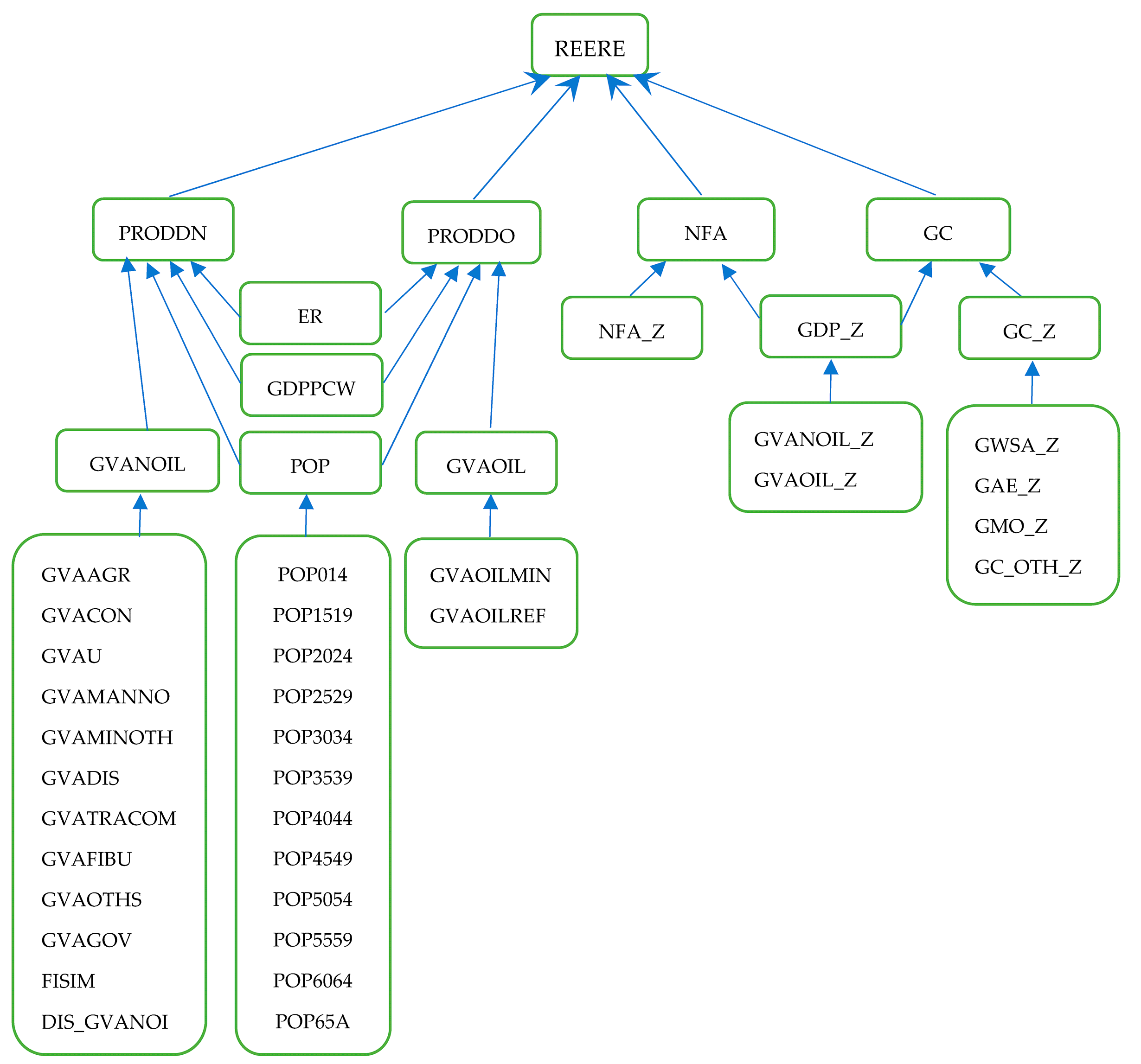
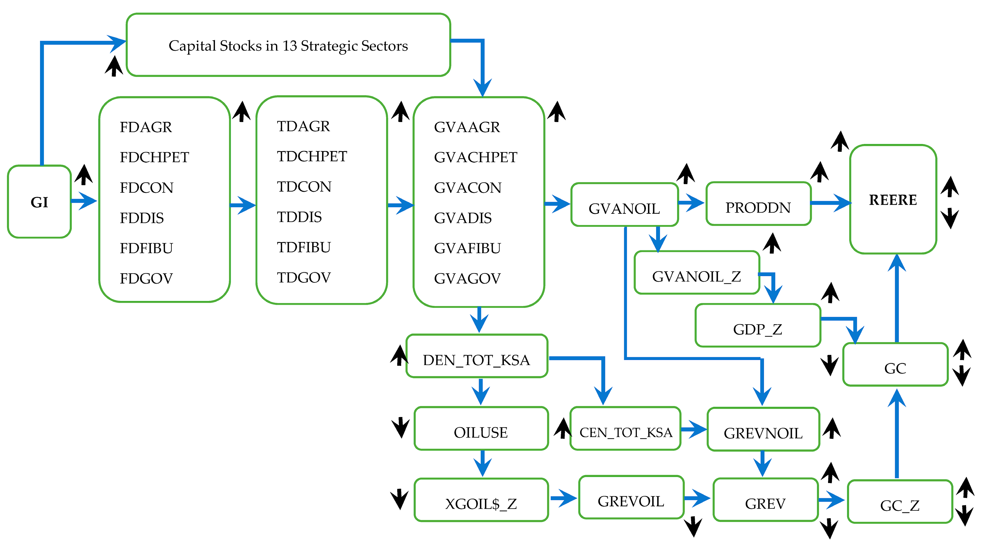
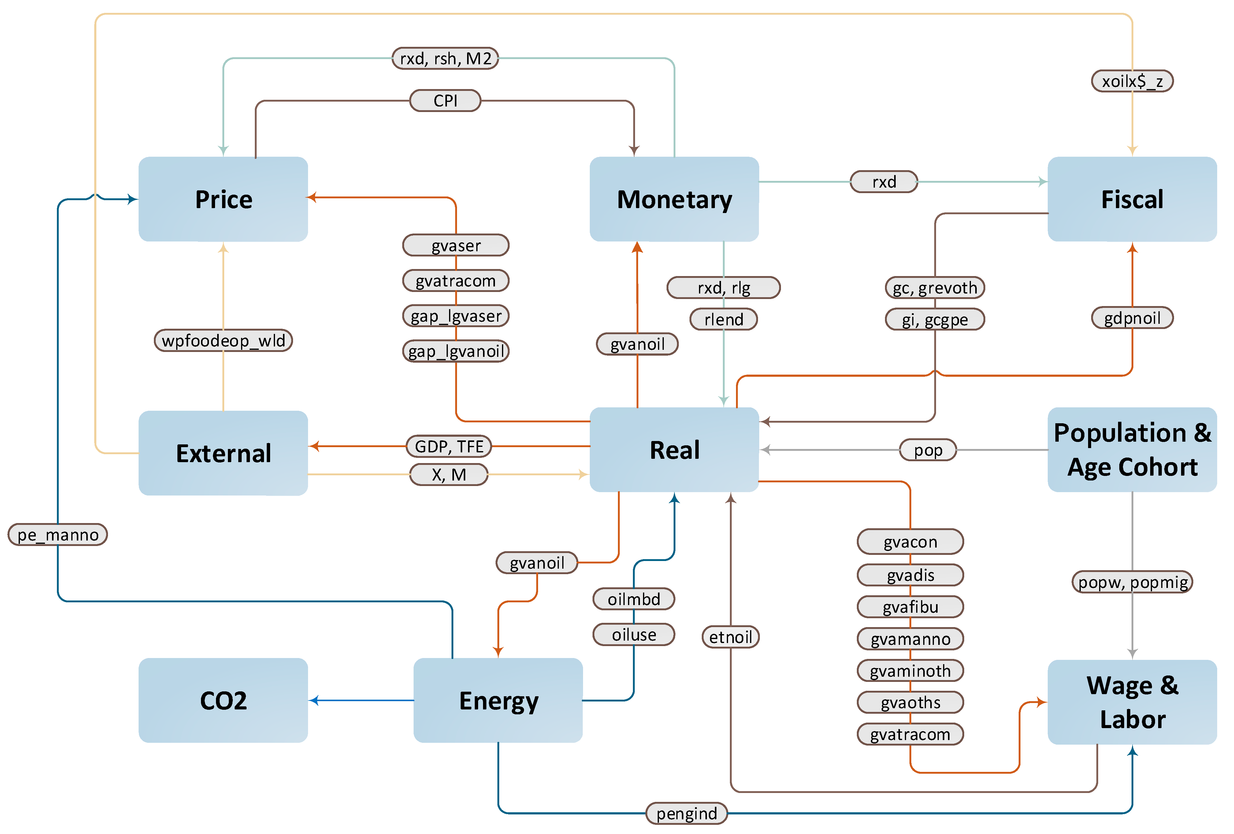
8.1. Brief Overview of the KGEMM and REERE Linkages

The KGEMM is a policy tool that assesses the impacts of internal decisions made by Saudi policymakers and changes in the global economy on Saudi Arabia’s economic, energy, and environmental relations at both aggregate and disaggregate levels [22,23]. The KGEMM is a general equilibrium, energy- and environment-sector augmented model. It is also a hybrid macroeconometric model in two senses. First, it combines theory-driven and data-driven approaches, as these types of models perform better than purely theory-based models (e.g., dynamic stochastic general equilibrium models or computable general equilibrium models) and purely data-based models (e.g., unrestricted VAR, AR, ARIMA models), as discussed in the literature (see [98,99,100,101,102,103,104,105,106,107,108]). Second, the KGEMM incorporates input–output intermediate demand, final demand, and total demand relationships into the macroeconomic framework. This allows the KGEMM to evaluate the disaggregated effects of demand components on economic, energy, and environmental indicators. Of course, as with any other model, the KGEMM also has drawbacks. For example, large-scale macroeconometric models such as the KGEMM are highly dependent on data availability, updates and revisions and the associated re-estimations, which also requires a dedicated group of modelers. We briefly describe additional features of the KGEMM in Appendix E. The version of the KGEMM employed here differs from that documented by [22] in the following ways. First, the relationship for the equilibrium real effective exchange rate (REERE in Equation (3)) developed in this study has been incorporated into the KGEMM framework. This was done to fulfill the aim of the simulations in this paper and other research and policy analyses in the future. Instead of considering the estimated coefficients from one of the four estimated REER equations in Table 3 and Table 4, we took the average of the estimated coefficients across the methods in forming the REERE identity. The advantage of this combined approach is that it takes into consideration information from all four estimated equations using different methods. The incorporation of the REERE identity was successful, as the KGEMM was solved consistently. Second, the data have been updated, and most of the behavioral equations have been re-estimated through 2019. Third, the projections account for the impacts of COVID-19 and the low oil price environment and post-COVID-19 recovery. These and other changes in the KGEMM have been documented by [23].

Figure 4 illustrates the first-round (Equation (2)) and second-round linkages of REER-based competitiveness in the KGEMM framework. In Section 3, we describe the relationships between REER-based competitiveness (REERE) and its selected determinants. In Section 4, we then define these determinants—namely, productivity differentials in the non-oil sector (PRODDN) and oil sector (PRODDO) with respect to the rest of the world, as well as net foreign assets (NFA) and government consumption (GC). Hence, we do not discuss these again here.

Figure 4 further illustrates that the value added in the non-oil sector (GVANOIL) is the sum of the value added by 10 non-oil activities, including agriculture (GVAAGR), non-oil manufacturing (GVAMANNO), construction (GVACON), distribution (GVADIS), and public services (GVAGOV). Financial intermediaries, in million Riyal, at 2010 prices (FISIM) and the discrepancy term (DIS_GVANOIL) are also included in the GVANOIL identity to make it balanced. Definitions of the other non-oil economic activity sectors in Figure 4 can be found in [22,23]. Value added by the oil sector (GVAOIL) is the sum of value added by oil mining (GVAOILMIN) and oil refinery (GVAOILREF) activities. The total population, a component of productivity, is the sum of 12 population age groups, from children aged 0–14 years (POP014) to those over age 65 (POP65A). The nominal gross domestic product (GDP_Z), which feeds into NFA and GC in Equation (3), is the sum of the nominal value added in the non-oil sectors (GVANOIL_Z), nominal value added in the oil sector (GVAOIL_Z), and nominal value added by import taxes (GVANIT_Z). Nominal government consumption (GC_Z) is the sum of government wages, salaries, and allowances (GWSA_Z); government administrative expenses (GAE_Z); government maintenance operations (GMO_Z), and other government consumption (GC_OTH_Z), all in nominal terms. To ease interpretation, we econometrically estimated sectoral activities as functions of the energy demand of these activities and the total demand for these activities, except for oil mining (GVAOILMIN), which follows OPEC production agreements and other changes in the international energy markets (see, e.g., [109,110,111]). Total demand is the sum of intermediate demand and final demand. All three are input–output components. Intermediate demand represents interactions among all economic activities, whereas final demand expresses the impacts of final demand elements—that is, government and private investment and consumption, as well as exports categorized as oil goods, non-oil goods, and services—on economic activities. Details of these and other relationships can be found in [22].

8.2. Assumptions for the Simulations and Policy Context

We compared two scenarios: a business-as-usual (BaU) scenario, which simulates the Saudi economy moving into the future and is in line with the KGEMM reference case and a policy scenario (S1), which simulates what will happen to the REER-based competitiveness if the Saudi government implements the initiatives outlined in the PIF Program (2021–2025). Established in 1971, the PIF, one of the leading government agencies in Saudi Arabia, is actively engaged in implementing Saudi Vision 2030 initiatives and achieving its targets. In 2017, the PIF Program (2018–2020) was launched; it was followed by the PIF Program (2021–2025) in 2021. One of the initiatives of the latest program is to invest 150 billion SAR into the Saudi economy each year [24]. To achieve economic goals and support the sustainable development of the national economy, the PIF identified 13 strategic sectors. These are renewables and utilities; aerospace and defense; automotives; transportation and logistics; food and agriculture; construction and building components and services; entertainment, leisure, and sports; financial services; real estate; metals and mining; healthcare; consumer goods and retail; and telecoms, media, and technology [24]. Furthermore, Ref. [24] describes the initiatives, opportunities, progress, and direct strategic objectives that the PIF has comprehensively established for each of these sectors.

To this end, in S1, we simulate the KGEMM to examine what will happen to the Saudi Arabian REER-based competitiveness if government investments increase by 150 billion SAR each year from 2021 to 2025 beyond the projected values in the BaU scenario. We could provide more detailed policy insights if we were able to simulate the effects of disaggregated investments in the strategic sectors mentioned above. However, we could not find the breakdown of investments by these sectors for 2021–2025. This presents an opportunity to conduct an interesting and useful study when such a breakdown becomes available in the future. Obviously, investment is a key driver of economic development, including productivity growth. Therefore, this scenario analysis provides policymakers with useful insights regarding potential improvements in competitiveness associated with public investments. Two aspects are worth noting: (i) we simulated the impact of the PIF investments through government investments (GI) and (ii) this is not the investment from the government budget but from the PIF. A dedicated analysis of import substitution and local content is beyond the scope of this study. Figure 5 illustrates the projected values of government investments for both scenarios (i.e., BaU and S1).

The KGEMM reference case (BaU) projects that government investments will increase from 133.23 billion SAR in 2020 to 143.32 billion SAR in 2025 (red line in Figure 5). Such a projection can be considered reasonable, given that the share of the GDP attributed to government investments was, on average, approximately 6% from 1970 to 2020 and approximately 5% in 2019 and 2020, and they are predicted to remain steady at approximately 5% from 2021 to 2025. If the PIF strategy is implemented, government investments are projected to increase by 150 billion SAR each year in S1 compared to the BaU scenario (blue line in Figure 5). Assumptions about other variables, as well as technical details of the model and simulations, can be obtained from the authors upon request. Also, it is beyond the scope of this paper to provide projected values for all variables, as the KGEMM contains more than 800 variables.

Figure 6 illustrates the main transmission channel of the impact of government investment on REER-based competitiveness in the KGEMM framework. We call it the main transmission channel because there are also other channels through which public investment impacts the REERE, although such channels are very weak. For example, public investments also increase the value added in the oil refinery sector, which in turn leads to a very small increase in the productivity differential of the oil sector. As mentioned above, government investment (GI) is a component of the final demand (FD) for each economic activity sector, which in turn is a component of the total demand (TD) by sector. These TD components (together with the energy demand) serve as the explanatory variable in the econometric equation of the value added of economic activity sectors, which are aggregated into the value added in the non-oil sector (GVANOIL) and the value added in the oil sector (GVAOIL). This is the demand-side effect of GI. The supply-side effect of GI on GVANOIL passes through the capital stock-production channel. Precisely, as the upper part of Figure 6 illustrates, an increase in GI directed to the 13 strategic sectors identified by the PIF expands their capital stock and thus production, which amounts to the overall non-oil value added, i.e., GVANOIL. Finally, GVANOIL is a component of the productivity differential in the non-oil sector with respect to the rest of the world (PRODDN), as expressed in the Data section. The latter is one of the determinants of external price competitiveness (REERE), as Equation (3) expresses. Thus, expanded government investments due to the PIF will improve external price competitiveness by increasing productivity in the non-oil sector.

Moreover, Figure 6 illustrates that expanding economic activities, driven by increased public investments, will result in more domestic energy consumption (DEN_TOT_KSA and OILUSE will rise). This will leave less crude and refined oil available for export (i.e., XGOIL$_Z decreases). This is because Saudi Arabian oil production is subject to OPEC production agreements (see, e.g., [110]), and renewables constitute a very small share (consistently 0.01% from 1996 to 2015) of the Kingdom’s energy mix (International Energy Agency data; [112]). We assume that the increased energy demand caused by growing economic activity is fulfilled by fossil fuels, as the share of renewables is assumed to be the same in both scenarios for the simulation period. However, the KGEMM framework allows us to change this assumption and assume a higher share of renewables in meeting the total energy demand in the economy, which can be done in future research (see the third out of sample simulation in [23]). As a result, government oil revenues (GREVOIL) will decline in S1 compared to BaU, assuming that the export prices of crude and refined oil remain the same in both scenarios. The government’s non-oil revenues (GREVNOIL) will increase as domestic energy sales (CEN_TOT_KSA) and collections from economic activities, such as taxes on income, profits, and capital gains, increase. As a result, the total government revenues (GREV) can decrease with oil revenues and increase with non-oil revenues. These ambiguous (positive and negative) effects will be transmitted to government expenditures, including government consumption (GC_Z), as it is financed by government revenues. Increased value added by the non-oil sector (GVANOIL) leads to an increase in nominal non-oil value added (GVANOIL_Z) and thereby nominal GDP (GDP_Z). The increase in the latter causes government consumption (GC) to shrink as it is the denominator in the calculation (see the Data section). Thus, the impact of government consumption (GC) on external price competitiveness (REERE) is ambiguous. However, it is likely that the negative impact of the oil revenue decline would overshadow the positive effect of a non-oil revenue increase because the oil sector accounts for a large share of the total government revenues (see, e.g., [11,113]).

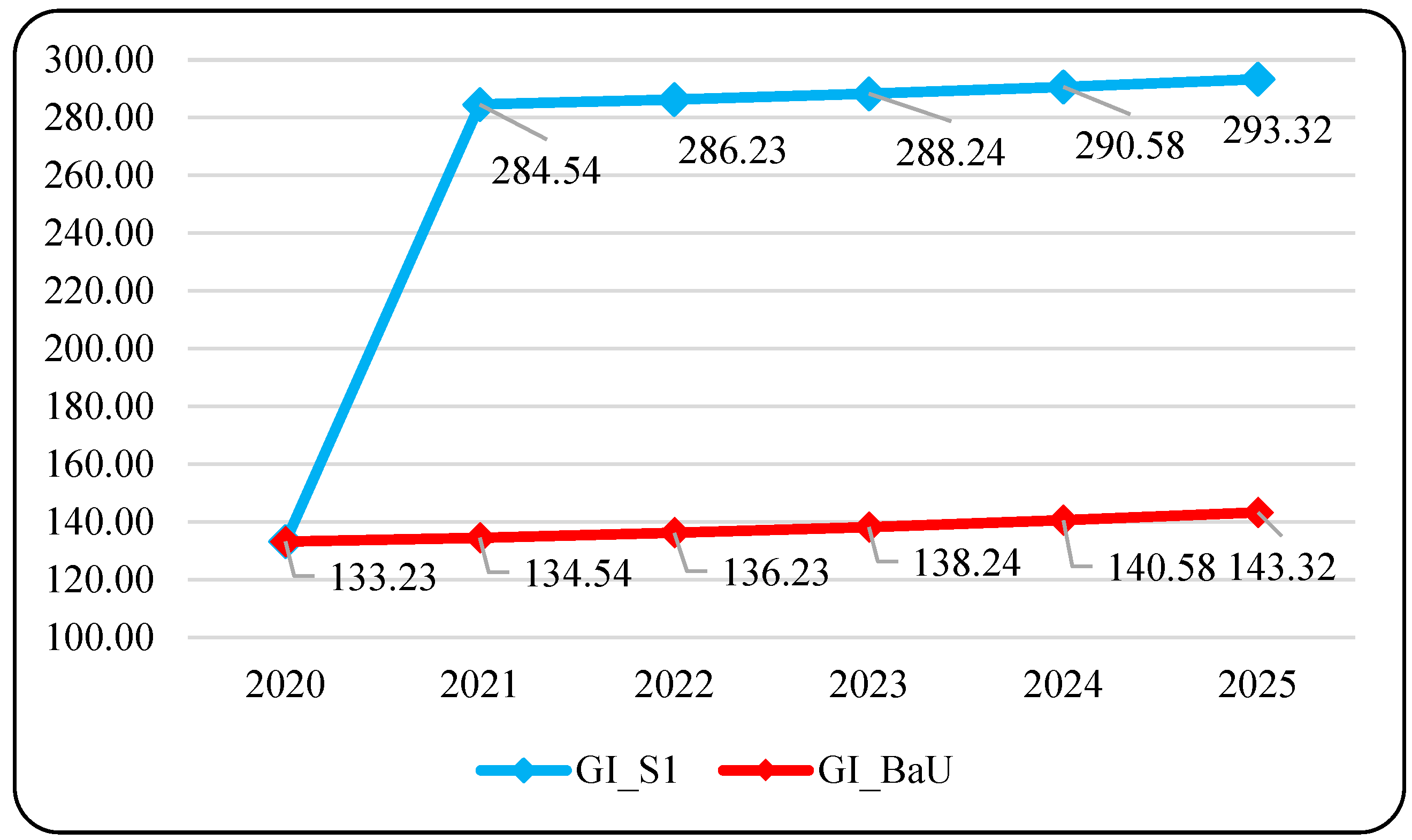
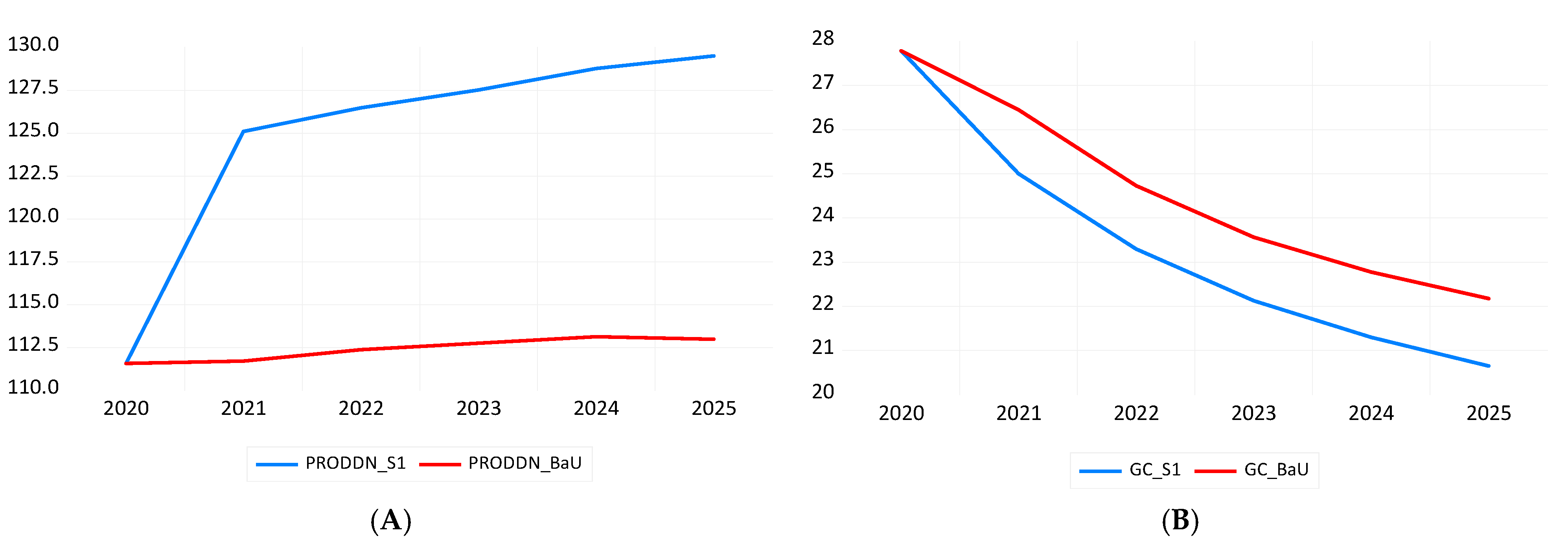
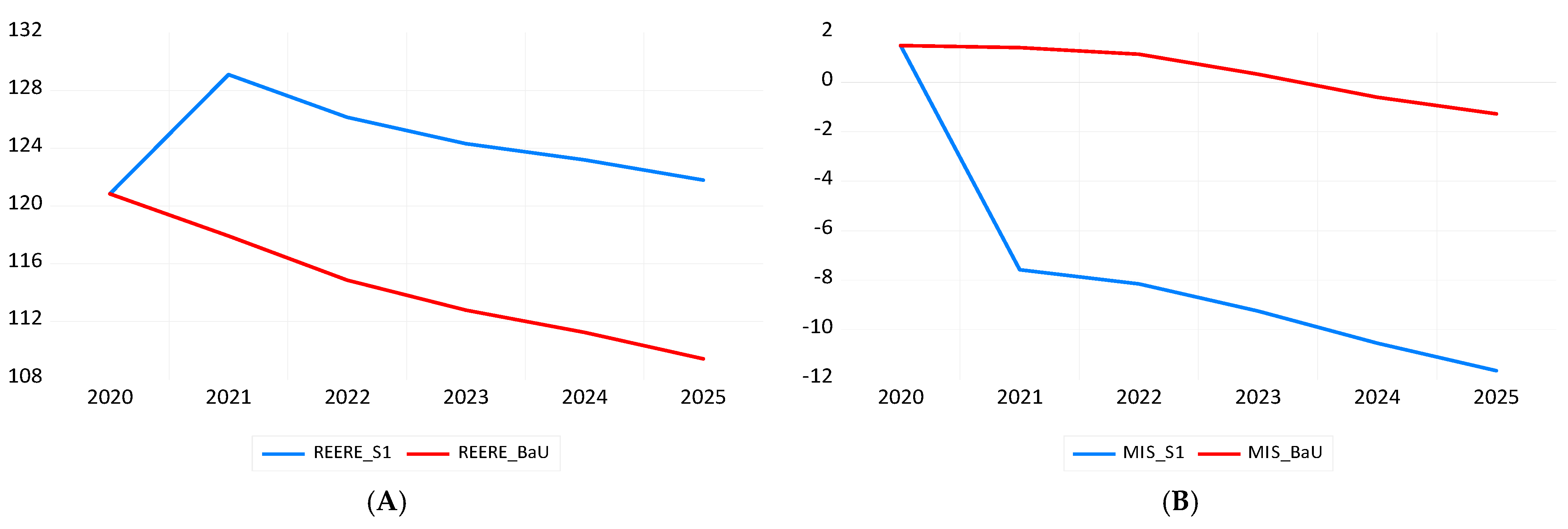
8.3. Results of the Projections

Figure 7 illustrates the projected paths of the non-oil productivity differential and the size of government consumption—two direct determinants of the REER (see Equation (2)). As can be expected from the associated discussion, the productivity differential in the non-oil sector increases, while the government consumption size decreases, in S1 compared to BaU because of increased government investments (See Figure 7). Inspection of the model simulation results reveals that increases in the productivity differential of the non-oil sector (PRODDN) are entirely driven by expansions in the sector’s economic activities (GVANOIL) given that the values of its other components—that is, the bilateral exchange rate (ER), world productivity (GDPPCW), and population (POP)—do not change from BaU to S1. Numerically, increases in value added by the non-oil sector in S1, compared to BaU, are very similar to the projected increases in the productivity differential from 2021 to 2025 shown in

Table 6. Deviations of S1 from BaU, percentage change.

Year	GI	PRODDN	REERE
2021	111.49	11.98	9.48
2022	110.11	12.54	9.84
2023	108.50	13.09	10.23
2024	106.70	13.82	10.75
2025	104.66	14.62	11.33
Average	108.29	13.21	10.33
Implied elasticity		0.10	0.12

Source: Simulation results conducted by the authors.

. This implies that increased government investment leads to increased value added of the non-oil sector. Regarding the government consumption size (GC), declines in S1 illustrated in Figure 7 are mainly driven by increases in nominal GDP. In other words, the size of government consumption decreases as non-oil economic activity and the resulting GDP and nominal GDP expand. The simulation results show that the declines in nominal government consumption (GC_Z) in S1 are quite small (i.e., 0.1% in 2021, rising to only 0.3% in 2025) compared to those in BaU.

Figure 8A illustrates that the net effect of these two main drivers (PRODDN and GC) on REER-based competitiveness is positive, as its values in S1 are higher than those in the BaU scenario. The REER establishes higher equilibrium levels because of increases in government investments over the next five years. This implies that the external competitiveness of the Kingdom rises in S1 compared to BaU. The simulation results are consistent with the theoretically predicted relationships between competitiveness, productivity, government consumption, and investment, as well as the results of the empirical estimations discussed in the previous section.

Figure 8B illustrates the SAR misalignments in both scenarios. It is apparent from the graph that without additional public investments in the economy, misalignments (i.e., deviations of the observed REER from its equilibrium level, determined by domestic and external fundamentals) show a minimal change from 1.4% in 2021 to −1.3% in 2025, as the red line illustrates. Recall that even in-sample misalignments were in an acceptable range, particularly in recent years (see Figure 3). These misalignment results, from both the estimations and simulations, show that the Kingdom’s exchange rate and monetary policies have been quite successful. The actual/observed REER deviated from its equilibrium path only slightly. When the PIF makes additional investments in the economy in S1, the fundamentals of the equilibrium exchange rate (mainly the productivity differential in the non-oil sector) increase. This leads to larger misalignments compared to BaU (see Figure 8B). In other words, driven mainly by productivity increases, the equilibrium path of the REER increases faster than the observable path of the REER, leading to higher level of competitiveness. Numerically, misalignments in S1 change from −7.6% in 2021 to −11.7% in 2025. Note, however, that such misalignments are not harmful, as they are driven mainly by productivity growth as discussed in the previous sections.

Table 6 reports numerical values from the simulations for the selected variables. We added the productivity differential in the non-oil sector (PRODDN) to the table as the development of the sector is a key goal in Saudi Vision 2030.

Table 6 documents the percentage deviations of the S1 values of government investment, the non-oil productivity differential, and REER-based competitiveness from BaU values. On average, a 108% increase in government investment translates into a 13% increase in productivity, which leads to a 10% appreciation of the equilibrium REER. To this end, the implied average elasticities of the non-oil productivity differential and equilibrium REER with respect to government investments are 0.10 and 0.12, respectively. This out-of-sample elasticity of 0.10 is quite reasonable given that the in-sample (1971–2020) average elasticity of the non-oil productivity differential with respect to government investments is calculated as 0.11 (calculated as the average value of the elasticities, i.e., the ratios of the growth rates of the non-oil productivity differential to the growth rates of government investments in each year for the period 1971–2020). As noted above, two components of the non-oil productivity differential—namely, the bilateral nominal exchange rate of USD to SAR (ER) and productivity in the rest of the world (GDPPCW)—are treated as exogenous in the simulations (i.e., their values do not change from BaU to S1). Moreover, projected population values are the same in both scenarios, even though the KGEMM treats the total population as an endogenous variable (see Figure 4). Thus, it is the non-oil value added that transmits public investment effects to the productivity differential between the non-oil sector and the rest of the world (PRODDN). We further investigated the simulation results for non-oil value added (GVANOIL) and found that its implied elasticity with respect to government investment for 2021–2025 is 0.12 (calculated as the average value of the ratios of the percentage deviations of GVANOIL and GI in S1 from their respective values in BaU. See [114] inter alia). This magnitude seems reasonable given that the in-sample average elasticity is calculated to be 0.15 for 1971–2020. Thus, it can be concluded that government investments lead to increased value added and increased productivity in the non-oil sector, thereby increasing the equilibrium level of the REER and Saudi Arabia’s external price competitiveness.

As external competitiveness improves because of PIF investments in S1 compared to BaU, Saudi Arabia’s exports are boosted. Specifically, non-oil exports increase by 14.7% on average, leading to a 0.8% increase in total exports, on average, over 2021–2025, in S1 compared to BaU. At the same time, PIF investments lead to an increase in total imports by an average of 9.9% over the 2021–2025 period in S1 compared to BaU. This increase in imports leads to a deterioration in the trade balance by an average of 12% in S1 compared to BaU. To avoid a deterioration in the trade balance, or at least reduce its magnitude, one option that authorities may wish to consider is to reduce imports by substituting them, where possible, with domestically produced goods and services. The substitution of imports with domestic production is important for local content development and thus for the diversification of the Saudi economy, the main goal of Saudi Vision 2030.

9. Conclusions and Policy Insights

Among other targets, Saudi Vision 2030 aims to improve Saudi Arabia’s ranking on the Global Competitiveness Index from 25 in 2015–2016 to within the top 10 by 2030. It also aims to increase the share of non-oil exports in the non-oil GDP from 16% in 2016 to 50% by 2030. Accomplishing these goals requires considerable improvements in Saudi Arabia’s competitiveness. This necessitates, among other aspects, an investigation to help decision-makers to better comprehend the driving forces of Saudi competitiveness.

To this end, we examined the REER as a measure of external price competitiveness and investigated both theoretically predicted and country-specific determinants. Our decision to examine the REER was rooted in literature, as previous studies have shown that it captures both domestic and global changes. We developed a novel modeling framework for REER-based competitiveness to provide policymakers with broader information regarding Saudi Arabia’s historical and projected competitiveness. To obtain robust estimates and derive well-grounded policy insights, we employed different unit root and cointegration tests as well as estimation methods. As a further robustness check, we expanded Equation (2) with additional variables to examine whether those variables provide additional information to explain the behavior of the REER. Lastly, we incorporated the estimated REER relationships into the KGEMM, a full/general equilibrium macroeconometric model, and conducted a policy scenario analysis for 2021–2025 to quantify the competitiveness effects of the PIF’s new strategy of investing in 13 strategic sectors through the non-oil sector’s productivity.

We found that Saudi external price competitiveness is shaped mainly by the productivity differential of the non-oil sector, followed by government consumption, the productivity differential of the oil sector, and NFA. The in-sample misalignment analysis shows that the observed REER values remain quite close to the equilibrium values, except during abnormal periods. This means that the appreciation and depreciation from equilibrium values have remained within an acceptable range over the period of investigation. This may indicate that the Saudi Central Bank’s exchange rate policy was quite successful. The KGEMM scenario analysis shows that when the PIF makes additional investments in the economy, the fundamentals of the equilibrium exchange rate (primarily the value added and productivity differential of the non-oil sector) rise. Saudi external price competitiveness improves as a result. Accordingly, misalignments become larger compared to those in the reference (BaU) case. In other words, the equilibrium path of the REER (that is, Saudi Arabia’s competitiveness level) shifts upward.

We have derived few policy insights from this research. The main point that policymakers may wish to consider is that productivity growth in the non-oil sector is the main driver of Saudi Arabia’s external price competitiveness. Hence, initiatives that can boost this productivity should be implemented. The simulation results show that public investment is a promising initiative in this regard, and investments by the PIF are worth highlighting. Authorities also may consider increasing government consumption, which can lead to the appreciation of both the observed and equilibrium values of the REER. The extent to which this increase may undermine competitiveness depends on whether the observed values exceed the equilibrium values. Hence, policymakers should be updated regularly regarding REER misalignment. Additionally, with respect to government consumption and public investment spending, substituting imports with locally produced goods and services where possible should be considered. Increased local content would greatly contribute to diversifying the economy, which is the key policy strategy of Saudi Vision 2030. Another policy consideration relates to NFA, as our results show that a decrease in NFA leads to the appreciation of the REER. This result implies that attracting more foreign investment and other assets from the rest of the world may lead to technological development, an enhanced business environment, and an improvement in the economic, financial, and social infrastructure. However, it may also lower the country’s NFA position and thus appreciate the REER. The former may increase competitiveness. However, if appreciation causes the observed values of the REER to exceed its equilibrium value, competitiveness may be worsened. This, in turn, necessitates updating the decision-making process to account for this misalignment stance.

Of course, this study is not free of limitations, which can be addressed in future research. One of the limitations is that we used the world GDP per capita in the construction of productivity differentials for the oil and non-oil sectors. Instead of this, one may wish to use the GDP per capita of Saudi Arabia’s main trading partners. Moreover, one may be interested in constructing world oil GDP per capita and world non-oil GDP per capita measures using the oil rent data from the World Bank database across all countries over the world, although such construction would be quite time-consuming. In addition, as an alternative measure, one may be interested in constructing a productivity differential using prices in Saudi Arabia (e.g., oil and non-oil prices) and those of the world (or in the main trading partners). Moreover, one may consider employment or labor force instead of the population in the construction of productivity measures. Furthermore, in the future, one can try to obtain data at a quarterly frequency (by either taking them from subscription-based data sources or interpolating the annual data) and use those data in the econometric estimations and testing to gain more efficiency, although this approach is debatable. Lastly, as the KGEMM is a publicly available modeling tool (https://apps.kapsarc.org/appboard/kgemm, accessed on 11 March 2023), one can extend this study by using it to simulate the competitiveness effects of other variables of interest or policy levers (such as localization targets, adjustments in the energy incentives, value-added tax, and expatriate levies).

References

1. Wysokińska, Z. Competitiveness and its relationships with productivity and sustainable development. Fibres Text. East. Eur. 2003, 11, 42. [Google Scholar]
2. Andreoni, V.; Miola, A. Competitiveness and Sustainable Developent Goals; Publications Office of the European Union: Luxembourg, 2016. [Google Scholar]
3. Kiseľáková, D.; Šofranková, B.; Čabinová, V.; Onuferová, E. Competitiveness and sustainable growth analysis of the EU countries with the use of Global Indexes’ methodology. Entrep. Sustain. 2018, 5, 581–599. [Google Scholar] [CrossRef] [PubMed] [Green Version]
4. Krstić, M.; Filipe, J.A.; Chavaglia, J. Higher Education as a Determinant of the Competitiveness and Sustainable Development of an Economy. Sustainability 2020, 12, 6607. [Google Scholar] [CrossRef]
5. Suranovic, S. International Trade: Theory and Policy; Saylor Foundation: New York, NY, USA, 2010. [Google Scholar]
6. Anyaehie, M.C.; Areji, A.C. Economic diversification for sustainable development n Nigeria. Open J. Political Sci. 2015, 5, 87. [Google Scholar] [CrossRef] [Green Version]
7. Krugman, P.R.; Obstfeld, M.; Melitz, M. International Economics: Theory and Policy, 10th ed.; Pearson Series in Economics: London, UK, 2015. [Google Scholar]
8. Mania, E.; Rieber, A. Product export diversification and sustainable economic growth in developing countries. Struct. Chang. Econ. Dyn. 2019, 51, 138–151. [Google Scholar] [CrossRef]
9. Xu, Z.; Li, Y.; Chau, S.N.; Dietz, T.; Li, C.; Wan, L.; Zhang, J. Impacts of international trade on global sustainable development. Nat. Sustain. 2020, 3, 964–971. [Google Scholar] [CrossRef]
10. Beutel, J. Economic diversification and sustainable development of GCC countries. In When Can Oil Economies Be Deemed Sustainable? Palgrave Macmillan: Singapore, 2021; pp. 99–151. [Google Scholar]
11. Hasanov, F.; Javid, M.; Joutz, F.L. Saudi Non-oil Exports Before and After COVID-19: Historical Impacts of Determinants and Scenario Analysis. Sustainability 2022, 14, 2379. [Google Scholar] [CrossRef]
12. Balassa, B. The Purchasing Power Parity Doctrine: A Reappraisal. J. Political Econ. 1964, 72, 584–596. [Google Scholar] [CrossRef] [Green Version]
13. European Commission. Price and Cost Competitiveness: Technical Appendix; Directorate-General for Economic and Financial Affairs: Brussels, Belgium, 2002. [Google Scholar]
14. International Monetary Fund (IMF). n.d. What Is Real Effective Exchange Rate (REER)? Available online: http://datahelp.imf.org/knowledgebase/articles/537472-what-is-real-effective-exchange-rate-reer (accessed on 11 March 2023).
15. Nagayasu, J. Global and Country-specific Movements in Real Effective Exchange Rates: Implications for External Competitiveness. J. Int. Money Financ. 2017, 76, 88–105. [Google Scholar] [CrossRef]
16. Peters, D. Price Competitiveness in Central and Eastern Europe—A Case Study for Transition Economies; IMK Study No. 1/2010; IMK at the Hans Boeckler Foundation, Macroeconomic Policy Institute: Düsseldorf, Germany, 2010. [Google Scholar]
17. Samuelson, P.A. Theoretical Notes on Trade Problems. Rev. Econ. Stat. 1964, 46, 145–154. [Google Scholar] [CrossRef]
18. United Nations Conference on Trade and Development (UNCTAD). Development and Globalization: Facts and Figures; United Nations Conference on Trade and Development: New York, NY, USA, 2012; Available online: https://unctad.org/system/files/official-document/webgdsdsi2012d2_en.pdf (accessed on 11 March 2023).
19. Rodrik, D. The Real Exchange Rate and Economic Growth: Theory and Evidence; Working paper; Harvard University: Cambridge, MA, USA, 2007; Available online: http://citeseerx.ist.psu.edu/viewdoc/download?doi=10.1.1.554.1195&rep=rep1&type=pdf (accessed on 11 March 2023).
20. Alkhareif, R.M.; Barnett, W.A.; Qualls, J.H. Has the Dollar Peg Served the Saudi Economy Well? Int. Financ. Bank. 2017, 4, 145–162. [Google Scholar] [CrossRef] [Green Version]
21. Hasanov, F.J.; Al Rasasi, M.H.; Alsayaary, S.S.; Alfawzan, Z. Money demand under a fixed exchange rate regime: The case of Saudi Arabia. J. Appl. Econ. 2022, 25, 385–411. [Google Scholar] [CrossRef]
22. Hasanov, F.; Joutz, F.L.; Mikayilov, J.I.; Javid, M. KGEMM: A Macroeconometric Model for Saudi Arabia; KAPSARC Discussion Paper No. KS-2020-DP04; King Abdullah Petroleum Studies and Research Center: Riyadh, Saudi Arabia, 2020. [Google Scholar] [CrossRef] [Green Version]
23. Hasanov, F.; Joutz, F.L.; Mikayilov, J.I.; Javid, M. KGEMM: A Macroeconometric Model for Saudi Arabia; Springer: New York, NY, USA, 2023. [Google Scholar]
24. Public Investment Fund (PIF). Public Investment Fund Program 2021–2025. 2021. Available online: https://www.pif.gov.sa/VRP%202025%20Downloadables%20EN/PIFStrategy2021-2025-EN.pdf (accessed on 11 March 2023).
25. Beenstock, M.; Dalziel, A. The Demand for Energy in the UK: A General Equilibrium Analysis. Energy Econ. 1986, 8, 90–98. [Google Scholar] [CrossRef]
26. Bandara, J.S. Computable general equilibrium models for development policy analysis in LDCs. J. Econ. Surv. 1991, 5, 3–69. [Google Scholar] [CrossRef]
27. Beck, J.H. Distributive justice and the rules of the corporation: Partial versus general equilibrium analysis. Bus. Ethics Q. 2005, 15, 355–362. [Google Scholar] [CrossRef]
28. Thomsen, M.R. An Interactive Text for Food and Agricultural Marketing. 2018. Open Education Resource (OER) LibreTexts Project. Available online: https://LibreTexts.org (accessed on 11 March 2023).
29. Cusbert, T.; Kendall, E. Meet MARTIN, the RBA’s New Macroeconomic Model. Aust. Reserve Bank Bull. 2018, 31–44. [Google Scholar]
30. Hasanov, F. Theoretical Framework for Industrial Electricity Consumption Revisited: Empirical Analysis and Projections for Saudi Arabia; KAPSARC Discussion Paper No. KS-2019-DP66; King Abdullah Petroleum Studies and Research Center: Riyadh, Saudi Arabia, 2019. [Google Scholar] [CrossRef] [Green Version]
31. Ballantyne, A.; Cusbert, T.; Evans, R.; Guttmann, R.; Hambur, J.; Hamilton, A.; Kendall, E.; McCirick, R.; Nodari, G.; Rees, D.M. MARTIN Has Its Place: A Macroeconometric Model of the Australian Economy. Econ. Rec. 2020, 96, 225–251. [Google Scholar] [CrossRef] [Green Version]
32. Razek, N.H.A.; McQuinn, B. Saudi Arabia’s Currency Misalignment and International Competitiveness, Accounting for Geopolitical Risks and the Super-contango Oil Market. Resour. Policy 2021, 72, 102057. [Google Scholar] [CrossRef]
33. Aleisa, E.A.; Dibooĝlu, S. Sources of Real Exchange Rate Movements in Saudi Arabia. J. Econ. Financ. 2002, 26, 101–110. [Google Scholar] [CrossRef]
34. Habib, M.M.; Kalamova, M.M. Are There Oil Currencies? The Real Exchange Rate of Oil Exporting Countries; ECB Working Paper No. 839; European Central Bank: Frankfurt am Main, Germany, 2007. [Google Scholar] [CrossRef]
35. Altarturi, B.H.M.; Alshammri, A.A.; Hussin, T.M.T.I.T.; Saiti, B. Oil Price and Exchange Rates: A Wavelet Analysis for OPEC Members. Int. J. Energy Econ. Policy 2016, 6, 421–430. Available online: http://www.econjournals.com/index.php/ijeep/article/view/2253 (accessed on 11 March 2023).
36. Suliman, T.H.M.; Abid, M. The Impacts of Oil Price on Exchange Rates: Evidence from Saudi Arabia. Energy Explor. Exploit. 2020, 38, 2037–2058. [Google Scholar] [CrossRef]
37. Abdelaziz, M.; Chortareas, G.; Cipollini, A. Stock Prices, Exchange Rates, and Oil: Evidence from Middle East Oil-exporting Countries. Top. Middle East. Afr. Econ. 2008, 10, 1–27. Available online: http://meea.sites.luc.edu/volume10/PDFS/Paper%20by%20Abdelaziz&Chortareas&Cipollini.pdf (accessed on 11 March 2023).
38. Coudert, V.; Couharde, C. Currency Misalignments and Exchange Rate Regimes in Emerging and Developing Countries; CEPII Working Paper No. 2008-07; CEPII: Paris, France, 2008; Available online: http://www.cepii.fr/PDF_PUB/wp/2008/wp2008-07.pdf (accessed on 11 March 2023).
39. Mozayani, A.H.; Parvizi, S. Exchange Rate Misalignment in Oil Exporting Countries (OPEC): Focusing on Iran. Iran. Econ. Rev. 2016, 20, 261–376. [Google Scholar] [CrossRef]
40. Couharde, C.; Delatte, A.L.; Grekou, C.; Mignon, V.; Morvillier, F. EQCHANGE: A World Database on Actual and Equilibrium Effective Exchange Rates. Int. Econ. 2018, 156, 206–230. [Google Scholar] [CrossRef] [Green Version]
41. Grekou, C. EQCHANGE Annual Assessment 2018; CEPII Working Paper No. 2018-23; CEPII: Paris, France, 2018; Available online: http://www.cepii.fr/PDF_PUB/wp/2018/wp2018-23.pdf (accessed on 11 March 2023).
42. Mahraddika, W. Real exchange rate misalignments in developing countries: The role of exchange rate flexibility and capital account openness. Int. Econ. 2020, 163, 1–24. [Google Scholar] [CrossRef]
43. Guillaumin, C.; Boubakri, S.; Silanine, A. Do commodity price volatilities impact currency misalignments in commodity-exporting countries? Econ. Bull. 2020, 40, 1727–1739. [Google Scholar]
44. Lemaire, T. Civil Conflicts and Exchange Rate Misalignment: Evidence from MENA and Arab League Members; Economic Research Forum (ERF): Giza, Egypt, 2021. [Google Scholar]
45. Aman, Z.; Mallick, S.; Emlioglu, I. Currency regimes and external competitiveness: The role of institutions, trade agreements and monetary rameworks. J. Inst. Econ. 2022, 18, 399–428. [Google Scholar] [CrossRef]
46. del Carmen Ramos-Herrera, M.; Sosvilla-Rivero, S. Economic growth and deviations from the equilibrium exchange rate. Int. Rev. Econ. Financ. 2023, 86, 764–786. [Google Scholar] [CrossRef]
47. Ugurlu, E.N.; Razmi, A. Political economy of real exchange rate levels. J. Comp. Econ. 2023. [Google Scholar] [CrossRef]
48. Elsherif, M.; Mohieldin, M. The Dynamic Interaction of Exchange Rates and International Trade Flows in the MENA Region: GARCH Analysis; Economic Research Forum: Giza, Egypt, 2020. [Google Scholar]
49. Kasem, J.; Al-Gasaymeh, A. A Cointegration Analysis for the Validity of Purchasing Power Parity: Evidence from Middle East Countries. Int. J. Technol. Innov. Manag. 2022, 2. [Google Scholar] [CrossRef]
50. Leichter, J.; Mocci, C.; Pozzuoli, S. Measuring External Competitiveness: An Overview; Government of the Italian Republic, Ministry of Economy and Finance, Department of the Treasury Working Paper No. 2; Government of the Italian Republic: Rome, Italy, 2010. [CrossRef] [Green Version]
51. Comunale, M.; Mongelli, F.P. The Role of Real, Financial, Monetary and Institutional Factors in Tracking Growth. The World Economic Forum. 2020. Available online: https://www.weforum.org/agenda/2020/01/real-financial-monetary-institutional-factors-eu-growth/ (accessed on 11 March 2023).
52. Giordano, C. How Frequent a BEER? Assessing the Impact of Data Frequency on Real Exchange Rate Misalignment Estimation; Bank of Italy Occasional Paper 522; Bank of Italy: Rome, Italy, 2019. [Google Scholar]
53. Chinn, M.D. A Primer on Real Effective Exchange Rates: Determinants, Overvaluation, Trade Flows and Competitive Devaluation. Open Econ. Rev. 2006, 17, 115–143. [Google Scholar] [CrossRef] [Green Version]
54. Baffes, J.; Elbadawi, I.A.; S’ephen, A. O’Connell. Single-equation Estimation of the Equilibrium Real Exchange Rate. In Exchange Rate Misalignment Concepts and Measurement for Developing Countries; Hinkle, L.E., Montiel, P.J., Eds.; Oxford University Press: New York, NY, USA, 1999; pp. 405–466. [Google Scholar]
55. Clark, P.B. Concepts of Equilibrium Exchange Rates. In The Globalization of Markets; Stein, J.L., Ed.; Physica: Heidelberg, Germany, 1997; pp. 49–56. [Google Scholar] [CrossRef]
56. Clark, P.B.; MacDonald, R. Exchange Rates and Economic Fundamentals: A Methodological Comparison of BEERs and FEERs. In Equilibrium Exchange Rates; MacDonald, R., Stein, J.L., Eds.; Springer: New York, NY, USA, 1999; Volume 69, pp. 285–322. [Google Scholar] [CrossRef] [Green Version]
57. Clark, P.B.; MacDonald, R. Filtering the BEER: A Permanent and Transitory Decomposition. Glob. Financ. J. 2004, 15, 29–56. [Google Scholar] [CrossRef]
58. Lauro, B.; Schmitz, M. Euro Area Exchange Rate-based Competitiveness Indicators: A Comparison of Methodologies and Empirical Results. In Proceedings of the Sixth IFC Conference on Statistical Issues and Activities in a Changing Environment, Basel, Switzerland, 28–29 August 2012; Volume 36, pp. 325–339. Available online: https://econpapers.repec.org/bookchap/bisbisifc/36-21.htm (accessed on 11 March 2023).
59. Fidora, M.; Giordano, C.; Schmitz, M. Real Exchange Rate Misalignments in the Euro Area. Open Econ. Rev. 2021, 32, 71–107. [Google Scholar] [CrossRef]
60. Alshehabi, O.H.; Ding, S. Estimating Equilibrium Exchange Rates for Armenia and Georgia; IMF Working Paper No. 08/110; International Monetary Fund: Washington, DC, USA, 2008. [Google Scholar]
61. Javed, S.A.; Ali, W.; Ahmed, V. Exchange Rate and External Competitiveness: A Case of Pakistan; SDPI Monetary Policy Brief, Policy Paper No. 41; SDPI: Islamabad, Pakistan, 2016. [Google Scholar] [CrossRef]
62. Orszaghova, L.; Savelin, L.; Schudel, W. External Competitiveness of EU Candidate Countries; ECB Occasional Paper No. 141; European Central Bank: Frankfurt am Main, Germany, 2012; Available online: https://www.ecb.europa.eu/pub/pdf/scpops/ecbocp141.pdf (accessed on 11 March 2023).
63. Couharde, C.; Delatte, A.-L.; Grekou, C.; Mignon, V.; Morvillier, F. Measuring the Balassa-Samuelson effect: A guidance note on the RPROD database. Int. Econ. 2020, 161, 237–247. [Google Scholar] [CrossRef] [Green Version]
64. Couharde, C.; Grekou, C.; Mignon, V. MULTIPRIL, a new database on multilateral price levels and currency misalignments. Int. Econ. 2021, 165, 94–117. [Google Scholar] [CrossRef]
65. World Bank. World Development Indicators Database. 2021 Release. [Dataset]. 2021. Available online: https://datatopics.worldbank.org/world-development-indicators/ (accessed on 11 March 2023).
66. Chudik, A.; Mongardini, J. Search of Equilibrium: Estimating Equilibrium Real Exchange Rates in Sub-Saharan African Countries; IMF Working Paper No. 07/90; International Monetary Fund: Washington, DC, USA, 2007; ISBN 9781451866544. [Google Scholar]
67. Saudi Arabian Monetary Authority (SAMA). Yearly Statistics. Saudi Central Bank. 2018. Available online: https://www.sama.gov.sa/en-US/EconomicReports/Pages/YearlyStatistics.aspx (accessed on 11 March 2023).
68. Enders, W. Applied Econometrics Time Series, 5th ed.; Wiley: Hoboken, NJ, USA, 2015. [Google Scholar]
69. Pesaran, M.H.; Shin, Y. An Autoregressive Distributed Lag Modelling Approach to Cointegration Analysis; Cambridge Working Papers in Economics; Faculty of Economics, University of Cambridge: Cambridge, UK, 1995. [Google Scholar] [CrossRef]
70. Pesaran, M.H.; Shin, Y.; Smith, R.J. Bounds Testing Approaches to the Analysis of Level Relationships. J. Appl. Econom. 2001, 16, 289–326. [Google Scholar] [CrossRef]
71. Dickey, D.A.; Fuller, W.A. Distribution of the Estimators for Autoregressive Time Series with a Unit Root. J. Am. Stat. Assoc. 1979, 74, 427–431. [Google Scholar] [CrossRef]
72. Phillips, P.C.B.; Perron, P. Testing for a Unit Root in Time Series Regression. Biometrika 1988, 75, 335–346. [Google Scholar] [CrossRef]
73. Enders, W.; Lee, J. The Flexible Fourier Form and Dickey–Fuller Type Unit Root Tests. Econ. Lett. 2012, 117, 196–199. [Google Scholar] [CrossRef]
74. Perron, P. Testing for a Unit Root in a Time Series with a Changing Mean. J. Bus. Econ. Stat. 1990, 8, 153–162. [Google Scholar] [CrossRef]
75. Perron, P.; Vogelsang, T.J. Nonstationarity and Level Shifts with an Application to Purchasing Power Parity. J. Bus. Econ. Stat. 1992, 10, 301–320. [Google Scholar] [CrossRef]
76. Perron, P.; Vogelsang, T.J. Testing for a Unit Root in a Time Series with a Changing Mean: Corrections and Extensions. J. Bus. Econ. Stat. 1992, 10, 467–470. [Google Scholar] [CrossRef]
77. Vogelsang, T.J.; Perron, P. Additional Tests for a Unit Root Allowing for a Break in the Trend Function at an Unknown Time. Int. Econ. Rev. 1998, 39, 1073–1100. [Google Scholar] [CrossRef] [Green Version]
78. Enders, W.; Lee, J. A Unit Root Test Using a Fourier Series to Approximate Smooth Breaks. Oxf. Bull. Econ. Stat. 2012, 74, 574–599. [Google Scholar] [CrossRef] [Green Version]
79. Badinger, H. Austria’s Demand for International Reserves and Monetary Disequilibrium: The Case of a Small Open Economy with a Fixed Exchange Rate Regime. Economica 2004, 71, 39–55. [Google Scholar] [CrossRef]
80. Dibooglu, S.; Enders, W. Multiple Cointegrating Vectors and Structural Economic Models: An Application to the French Franc/US Dollar Exchange Rate. South. Econ. J. 1995, 61, 1098–1116. [Google Scholar] [CrossRef]
81. Ericsson, N.R.; MacKinnon, J.G. Distributions of error correction tests for cointegration. Econom. J. 2002, 5, 285–318. [Google Scholar] [CrossRef] [Green Version]
82. Johansen, S. Statistical Analysis of Cointegration Vectors. J. Econ. Dyn. Control 1988, 12, 231–254. [Google Scholar] [CrossRef]
83. Johansen, S. Cointegration in Partial Systems and the Efficiency of Single-equation Analysis. J. Econom. 1992, 52, 389–402. [Google Scholar] [CrossRef]
84. Johansen, S.; Juselius, K. Maximum Likelihood Estimation and Inference on Cointegration—With Applications to the Demand for Money. Oxf. Bull. Econ. Stat. 1990, 52, 169–210. [Google Scholar] [CrossRef]
85. Juselius, K. The Cointegrated VAR Methodology. In Oxford Research Encyclopedia of Economics and Finance; Oxford University Press: London, UK, 2006. [Google Scholar] [CrossRef]
86. Cheung, Y.-W.; Lai, K.S. Finite-sample Sizes of Johansen’s Likelihood Ratio Tests for Cointegration. Oxf. Bull. Econ. Stat. 1993, 55, 313–328. [Google Scholar] [CrossRef]
87. Reimers, H.-E. Comparisons of Tests for Multivariate Cointegration. Stat. Pap. 1992, 33, 335–359. [Google Scholar] [CrossRef]
88. Reinsel, G.C.; Ahn, S.K. Vector Autoregressive Models with Unit Roots and Reduced Rank Structure: Estimation, Likelihood Ratio Test, and Forecasting. J. Time Ser. Anal. 1992, 13, 353–375. [Google Scholar] [CrossRef]
89. Narayan, P.K. The Saving and Investment Nexus for China: Evidence from Cointegration Tests. Appl. Econ. 2005, 37, 1979–1990. [Google Scholar] [CrossRef]
90. MacKinnon, J.G. Numerical distribution functions for unit root and cointegration tests. J. Appl. Econom. 1996, 11, 601–618. [Google Scholar] [CrossRef]
91. MacKinnon, J.G.; Haug, A.A.; Michelis, L. Numerical Distribution Functions of Likelihood Ratio Tests for Cointegration. J. Appl. Econom. 1999, 14, 563–577. [Google Scholar] [CrossRef]
92. Gujarati, D.N.; Porter, D.C. Basic Econometrics, 5th ed.; McGraw-Hill: New York, NY, USA, 2009. [Google Scholar]
93. Meshulam, D.; Sanfey, P. The Determinants of Real Exchange Rates in Transition Economies; European Bank for Reconstruction and Development Working Paper Series (No. 228); European Bank for Reconstruction and Development: London, UK, 2019; Available online: https://www.ebrd.com/publications/working-papers/real-exchange-rates (accessed on 11 March 2023).
94. International Monetary Fund (IMF). Saudi Arabia: 2011 Article IV Consultation: Staff Report; Public Information Notice on the Executive Board Discussion; IMF Staff Country Reports No. 11/292; International Monetary Fund: Washington, DC, USA, 2011. [Google Scholar] [CrossRef]
95. Hasanov, F.J.; Liddle, B.; Mikayilov, J.I.; Bollino, C.A. How Total Factor Productivity Drives Long-run Energy Consumption in Saudi Arabia. In Energy and Environmental Strategies in the Era of Globalization; Shahbaz, M., Balsalobre, D., Eds.; Springer: New York, NY, USA, 2019; pp. 195–220. [Google Scholar]
96. Feenstra, R.C.; Inklaar, R.; Timmer, M.P. The Next Generation of the Penn World Table. Am. Econ. Rev. 2015, 105, 3150–3182. [Google Scholar] [CrossRef] [Green Version]
97. International Monetary Fund (IMF). Saudi Arabia: 2019 Article IV Consultation—Press Release and Staff Report; IMF Country Report No. 19/290; International Monetary Fund: Washington, DC, USA, 2019. [Google Scholar] [CrossRef] [Green Version]
98. Jelić, O.N.; Ravnik, R. Introducing Policy Analysis Croatian MAcroecoNometric Model (PACMAN); Croatian National Bank: Zagreb, Croatia, 2021. [Google Scholar]
99. Nikas, A.; Doukas, H.; Papandreou, A. A Detailed Overview and Consistent Classification of Climate-economy Models. In Understanding Risks and Uncertainties in Energy and Climate Policy; Doukas, H., Flamos, A., Lieu, J., Eds.; Springer: New York, NY, USA, 2019; pp. 1–54. [Google Scholar]
100. Blanchard, O. On the future of macroeconomic models. Oxf. Rev. Econ. Policy 2018, 34, 43–54. [Google Scholar] [CrossRef]
101. Blanchard, O. Do DSGE models have a future. In DSGE Models in the Conduct of Policy: Use as Intended; Gürkaynak, R.S., Tille, C., Eds.; CEPR Press: Brussels, Belgium, 2017; p. 93. [Google Scholar]
102. Hendry, D.F. Deciding between Alternative Approaches in Macroeconomics. Int. J. Forecast. 2018, 34, 119–135. [Google Scholar] [CrossRef]
103. Hendry, D.F.; Muellbauer, J.N.J. The Future of Macroeconomics: Macro Theory and Models at the Bank of England. Oxf. Rev. Econ. Policy 2018, 34, 287–328. [Google Scholar] [CrossRef] [Green Version]
104. Giacomini, R. Economic Theory and Forecasting: Lessons from the Literature. J. Econom. 2015, 18, C22–C41. [Google Scholar] [CrossRef] [Green Version]
105. Gürkaynak, R.S.; Tille, C. (Eds.) DSGE Models in the Conduct of Policy: Use as Intended; CEPR Press: Brussels, Belgium, 2017. [Google Scholar]
106. Gürkaynak, R.S.; Kısacıkoğlu, B.; Rossi, B. Do DSGE Models Forecast More Accurately Out-Of-Sample than VAR Models? Adv. Econom. 2013, 32, 27–79. [Google Scholar]
107. Pesaran, M.H.; Smith, R. Beyond the DSGE Straitjacket; CESifo Working Paper no. 3447; CESifo: Munich, Germany, 2011. [Google Scholar]
108. Wickens, M. Real business cycle analysis: A needed revolution in macroeconometrics. Econ. J. 1995, 433, 1637–1648. [Google Scholar] [CrossRef]
109. Kaufmann, R.K.; Dees, S.; Karadeloglou, P.; Sanchez, M. Does OPEC Matter? An Econometric Analysis of Oil Prices. Energy J. 2004, 25, 67–90. [Google Scholar] [CrossRef]
110. Kaufmann, R.K.; Bradford, A.; Belanger, L.H.; Mclaughlin, J.P.; Miki, Y. Determinants of OPEC Production: Implications for OPEC Behavior. Energy Econ. 2008, 30, 333–351. [Google Scholar] [CrossRef]
111. Wirl, F.; Kujundzic, A. The Impact of OPEC Conference Outcomes on World Oil Prices 1984–2001. Energy J. 2004, 25, 45–62. [Google Scholar] [CrossRef]
112. AlGhamdi, A. Saudi Arabia Energy Report; KAPSARC Discussion Paper No. KS–2020–DP25; King Abdullah Petroleum Studies and Research Center: Riyadh, Saudi Arabia, 2020. [Google Scholar]
113. Al Moneef, H.E.M.; Hasanov, F.J. Fiscal Multipliers for Saudi Arabia Revisited; KAPSARC Discussion Paper No. KS–2020–DP21; King Abdullah Petroleum Studies and Research Center: Riyadh, Saudi Arabia, 2020. [Google Scholar]
114. Musila, J.W. An Econometric Model of the Malawian Economy. Econ. Model. 2002, 19, 295–330. [Google Scholar] [CrossRef]
115. International Monetary Fund (IMF). Saudi Arabia: 2018 Article IV Consultation—Press Release and Staff Report; IMF Country Report No. 18/263; International Monetary Fund: Washington, DA, USA, 2018. [Google Scholar] [CrossRef]
116. Hasanov, F.J.; AlKathiri, N.; Alshahrani, S.A.; Alyamani, R. The impact of fiscal policy on non-oil GDP in Saudi Arabia. Appl. Econ. 2021, 54, 793–806. [Google Scholar] [CrossRef]
117. Al-Hamidy, A. Aspects of Fiscal/Debt Management and Monetary Policy Interaction: The Recent Experience of Saudi Arabia; BIS Paper No. 67v; Bank for International Settlements: Basel, Switzerland, 2012. [Google Scholar] [CrossRef] [Green Version]
118. Babetskii, I.; Égert, B. Equilibrium Exchange Rate in the Czech Republic: How Good is the Czech BEER? Czech J. Econ. Financ. 2005, 55, 232–252. [Google Scholar] [CrossRef] [Green Version]
119. Brixiova, Z.; Égert, B.; Essid, T.H.A. The Real Exchange Rate and External Competitiveness in Egypt, Morocco and Tunisia. Rev. Middle East Econ. Financ. 2014, 10, 25–51. [Google Scholar] [CrossRef] [Green Version]
120. Égert, B.; Lahrèche-Révil, A.; Lommatzsch, K. The Stock-flow Approach to the Real Exchange Rate of CEE Transition Economies; No. 2004-15; CEPII: Paris, France, 2004. [Google Scholar]
121. Al-Bassam, K.A. Money Demand and Supply in Saudi Arabia: An Empirical Analysis. Ph.D. Thesis, University of Leicester, Leicester, UK, 1990. [Google Scholar]
122. Al Rasasi, M.; Banafea, W. Estimating Money Demand Function in Saudi Arabia: Evidence from Cash in Advance Model; SAMA Working Paper: WP/18/4; Saudi Central Bank: Riyadh, Saudi Arabia, 2018. [Google Scholar]
123. Al Rasasi, M.H.; Qualls, J.H. Testing for Causality between Oil Prices and Money Supply in Saudi Arabia; SAMA Working Paper: WP/19/04; Saudi Central Bank: Riyadh, Saudi Arabia, 2019. [Google Scholar]
124. Chatah, M.B. A Monetary Framework for the Saudi Arabian Economy. Ph.D. Thesis, University of Texas at Austin, Austin, TX, USA, 1983. [Google Scholar]
125. Darrat, A.F. The Money Demand Relationship in Saudi Arabia: An Empirical Investigation. J. Econ. Stud. 1984, 11, 43–50. [Google Scholar] [CrossRef]
126. Darrat, A.F. The Demand for Money in Some Major OPEC Members: Regression Estimates and Stability Results. Appl. Econ. 1986, 18, 127–142. [Google Scholar] [CrossRef]
127. El Mallakh, R.; El Mallakh, D.H. Saudi Arabia: Energy, Developmental Planning, and Industrialization; Lexington Books: Lexington, MA, USA, 1982. [Google Scholar]
128. Al-Yousif, Y.K. Do Government Expenditures Inhibit or Promote Economic Growth: Some Empirical Evidence from Saudi Arabia. Indian Econ. J. 2000, 48, 92–96. [Google Scholar] [CrossRef]
129. Fasano, U.; Wang, Q. Fiscal Expenditure Policy and Non-oil Economic Growth: Evidence from GCC Countries; IMF Working Paper No. 2001-195; International Monetary Fund: Washington, DC, USA, 2001. [Google Scholar] [CrossRef]
130. Looney, R.E. Saudi Arabia’s Development Strategy: Comparative Advantage vs. Sustainable Growth; Defense Technical Information Center, Accession No. ADA528520; Naval Postgraduate School: Monterey, CA, USA, 1989. [Google Scholar]
131. Amano, R.A.; Van Norden, S. Exchange Rates and Oil Prices. Rev. Int. Econ. 1988, 6, 683–694. [Google Scholar] [CrossRef]
132. Chen, Y.; Rogoff, K. Commodity Currencies. J. Int. Econ. 2003, 60, 133–160. [Google Scholar] [CrossRef]
133. Ferraro, D.; Rogoff, K.; Rossi, B. Can Oil Prices Forecast Exchange Rates? An Empirical Analysis of the Relationship between Commodity Prices and Exchange Rates. J. Int. Money Financ. 2015, 54, 116–141. [Google Scholar] [CrossRef]
134. Benigno, G.; Thoenissen, C. Equilibrium Exchange Rates and Supply-side Performance. Econ. J. 2003, 113, C103–C124. [Google Scholar] [CrossRef]
135. MacDonald, R.; Ricci, L.A. Purchasing Power Parity and New Trade Theory; IMF Working Paper No. 02/32; International Monetary Fund: Washington, DC, USA, 2002. [Google Scholar] [CrossRef]
136. Alberola, E.; Navia, D. Equilibrium Exchange Rates in New EU Members: External Imbalances Versus Real Convergence. Rev. Dev. Econ. 2008, 12, 605–619. [Google Scholar] [CrossRef]
137. Alberola, E.; Navia, D. Equilibrium Exchange Rates in New EU Members: External Imbalances v. Real Convergence; Banco de España Working Paper No. 0708; Banco de España: Madrid, Spain, 2007. [Google Scholar]
138. Aglietta, M.; Baulant, C.; Coudert, V. Why the Euro Will Be Strong: An Approach Based on Equilibrium Exchange Rates. Rev. Econ. 1998, 49, 721–731. [Google Scholar]
139. Comunale, M. Current Account and Real Effective Exchange Rate Misalignments in Central Eastern EU Countries: An Update Using the Macroeconomic Balance Approach. Econ. Syst. 2018, 42, 414–436. [Google Scholar] [CrossRef]
140. Lommatzsch, K.; Tober, S. What is Behind the Real Appreciation of the Accession Countries’ Currencies? An Investigation of the PPI-based Real Exchange Rate. Econ. Syst. 2004, 28, 383–403. [Google Scholar] [CrossRef]
141. Burgess, R.; Fabrizio, S.; Xiao, Y. Competitiveness in the Baltics in the Run-up to EU Accession; IMF Country Report No. 03/114; International Monetary Fund: Washington, DC, USA, 2003. [Google Scholar]
142. Alonso-Gamo, P.; Fabrizio, S.; Kramarenko, V.; Wang, Q. Lithuania: History and Future of the Currency Board Arrangement; IMF Working Paper No. 127; International Monetary Fund: Washington, DC, USA, 2002. [Google Scholar]
143. Hemrit, W.; Benlagha, N. The Impact of Government Spending on Non-oil-GDP in Saudi Arabia (Multiplier Analysis). Int. J. Econ. Bus. Res. 2018, 15, 350–372. [Google Scholar] [CrossRef]
144. Oxford Economics Group. Oxford Economics Global Economic Model Database. March Release [Dataset]. 2021. Available online: https://www.oxfordeconomics.com/service/subscription-services/macro/global-economic-model/ (accessed on 11 March 2023).
145. Weyerstrass, K.; Neck, R.; Blueschke, D.; Majcen, B.; Srakar, A.; Verbič, M. SLOPOL10: A macroeconometric model for Slovenia. Econ. Bus. Rev. 2018, 20, 269–302. [Google Scholar] [CrossRef]
146. Khan, M.A.; ud Din, M. A Dynamic Macroeconometric Model of Pakistan’s Economy; Working Papers & Research Reports; Pakistan Institute of Development Economics: Islamabad, Pakistan, 2011. [Google Scholar]
147. Weyerstrass, K.; Neck, R. SLOPOL6: A macroeconometric model for Slovenia. Int. Bus. Econ. Res. J. 2007, 6, 81–94. [Google Scholar] [CrossRef]
148. Buenafe, S.W.; Reyes, C.M. Alternative Estimation Methodologies for Macro Model: ECM vs. OLS; PIDS Discussion Paper No. 2001-22; Philippine Institute for Development Studies (PIDS): Makati, Philippines, 2001. [Google Scholar]
149. Dreger, C.; Marcellino, M. A Macroeconometric Model for the Euro Economy. J. Policy Model. 2007, 29, 1–13. [Google Scholar] [CrossRef] [Green Version]
150. Welfe, W. Macroeconometric Models; Springer: New York, NY, USA, 2013. [Google Scholar]
151. Fair, R.C. An Analysis of the Accuracy of Four Macroeconometric Models. J. Political Econ. 1979, 87, 701–718. [Google Scholar] [CrossRef] [Green Version]
152. Fair, R.C. Testing Macroeconometric Models. Am. Econ. Rev. 1993, 83, 287–293. [Google Scholar]
153. Looney, R.E. Pre-revolutionary Iranian Economic Policy Making: An Optimal Control Based Assessment. Econ. Model. 1985, 2, 357–368. [Google Scholar] [CrossRef]
154. Looney, R.E. Socio-economic Tradeoffs in Saudi Arabia’s Third Five Year Plan (1980–1985). Socio-Econ. Plan. Sci. 1986, 20, 181–192. [Google Scholar] [CrossRef]
155. Looney, R.E. Saudi Arabia’s Fiscal Options: 1986–1992. Socio-Econ. Plan. Sci. 1988, 22, 109–123. [Google Scholar] [CrossRef]
Figure 1. Log levels and growth rates of the variables. (A) Log levels; (B) Growth rates. Source: Authors’ construction.
Sustainability 15 09011 g001aSustainability 15 09011 g001b
Figure 2. Actual and equilibrium REER series, 1980–2018. Scheme 2021 data, and authors’ estimations.
Sustainability 15 09011 g002
Figure 3. REER misalignment, %. Source: Authors’ calculation.
Sustainability 15 09011 g003
Figure 4. REER-based competitiveness linkages in KGEMM. Source: Authors’ construction.
Sustainability 15 09011 g004
Figure 5. Government investments (in billion SAR, 2010 prices). Source: Authors’ projections.
Sustainability 15 09011 g005
Figure 6. Transmission channel from government investments to competitiveness. Note: Sustainability 15 09011 i001, Sustainability 15 09011 i002, and Sustainability 15 09011 i003 indicate direction of impact, increase, and decrease, respectively. Source: Authors’ construction.
Sustainability 15 09011 g006
Figure 7. Projected paths of non-oil productivity differential and government consumption size. (A) PRODDN, BaU versus S1; (B) GC, BaU versus S1. Source: Authors’ projections.
Sustainability 15 09011 g007
Figure 8. Projected paths of competitiveness and misalignments. (A) REERE, BaU versus S1; (B) Misalignments, BaU versus S1. Source: Authors’ projections.
Sustainability 15 09011 g008