
Sustainability on Different Canola (Brassica napus L.) Cultivars by GGE Biplot Graphical Technique in Multi-Environment
 ,
,  , and
, and 
Abstract
:1. Introduction
2. Materials and Methods
2.1. Experiment Design
2.2. Analysis Method
- Evaluating together the grain yield and the stability of two cultivars at the same time
- Determine the most suitable genotype in each environment
- Evaluating the relationships between genotypes
- Ranking of genotypes based on the most suitable environment
- Classification of environments based on the most suitable genotype
- Appraising of relationships between environments using graphical analysis of GGE biplot
3. Results and Discussion
3.1. Variance Analysis
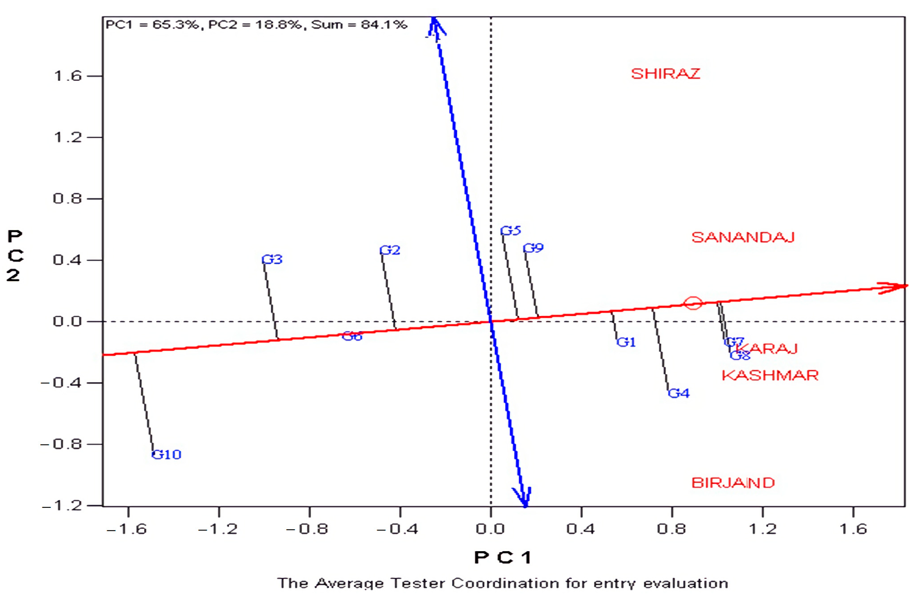
3.2. AEC View
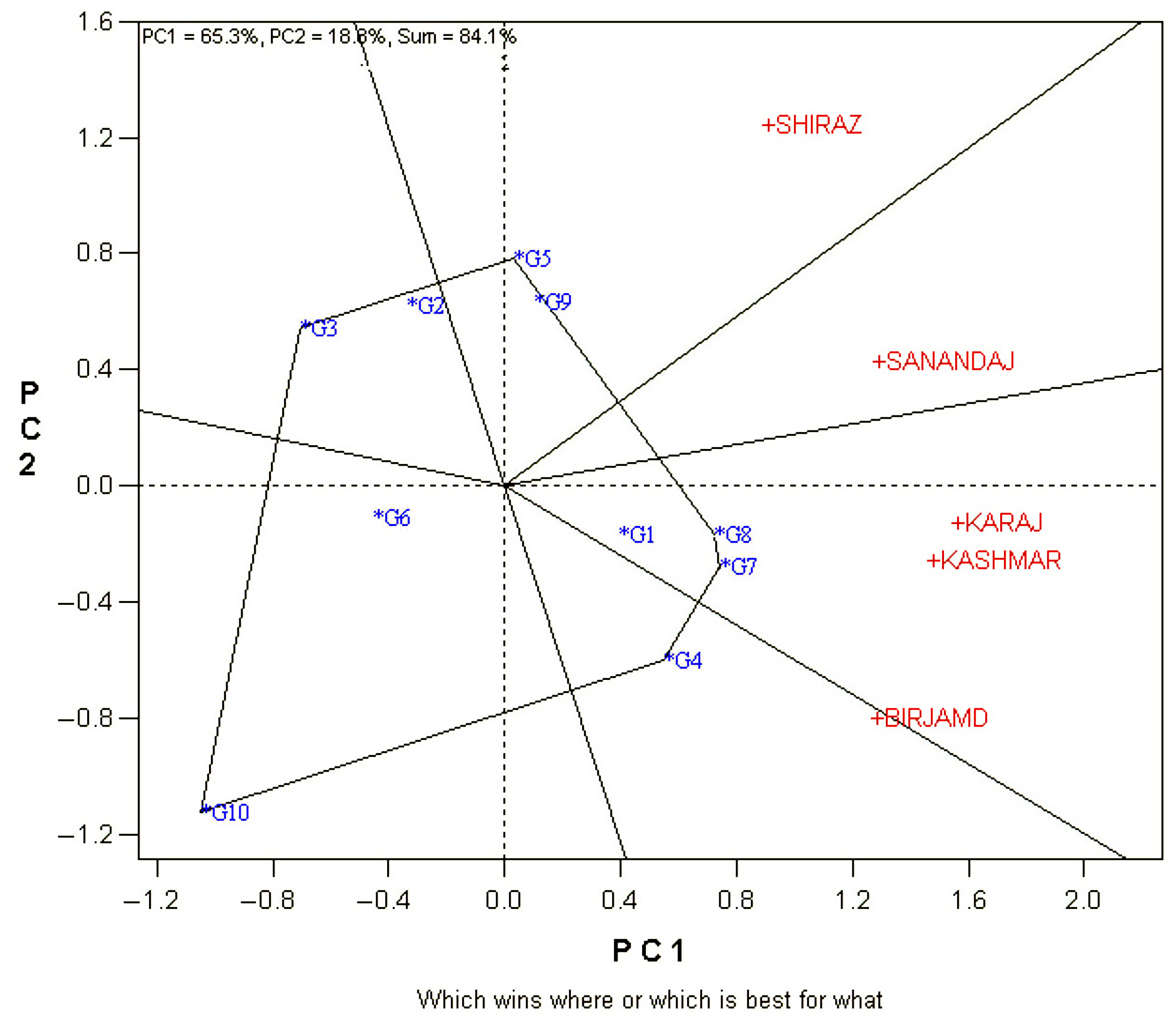
3.3. Polygon View
3.4. Genotype Grouping
3.5. Ranking of Genotypes Based on the Most Suitable Environment
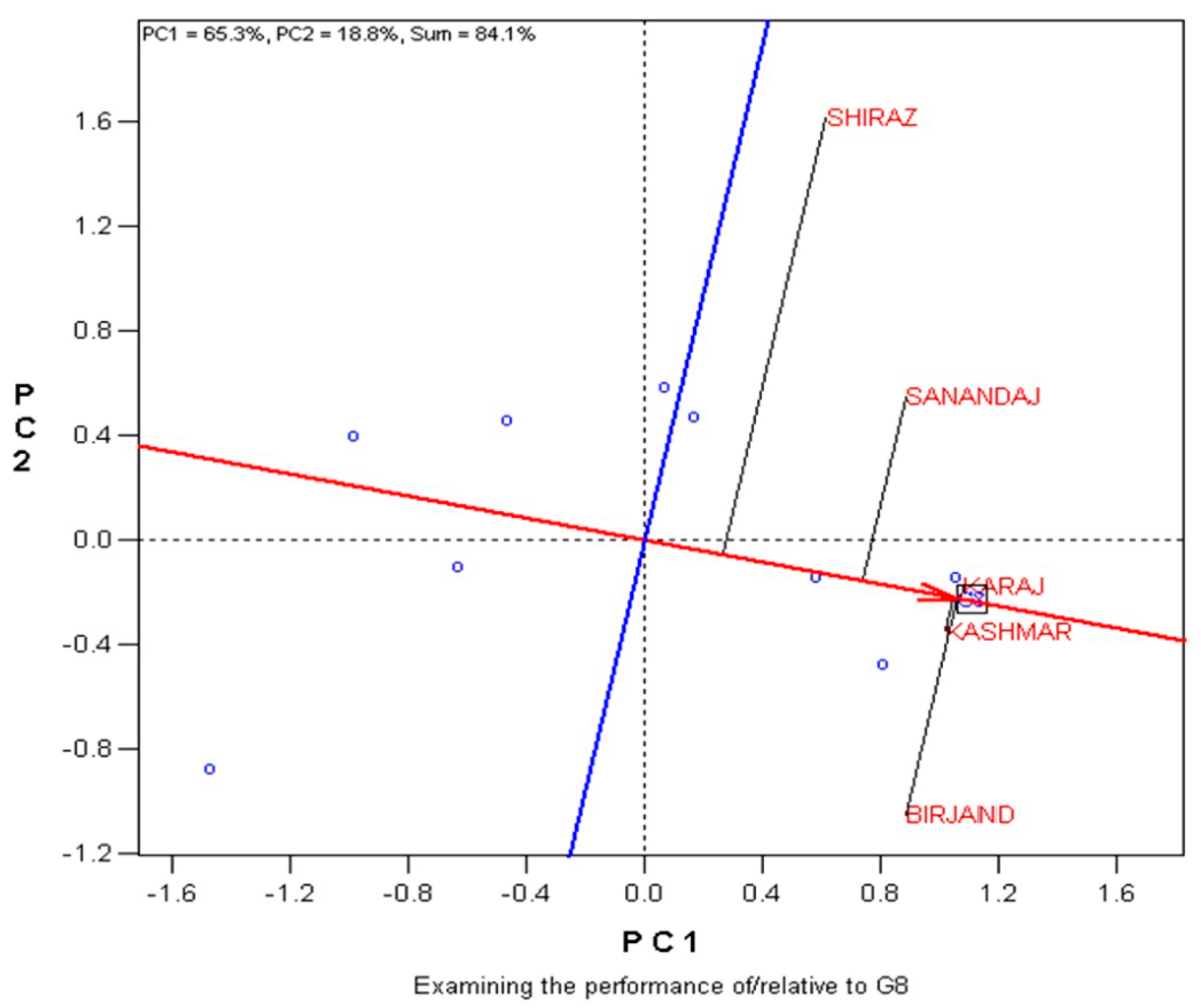
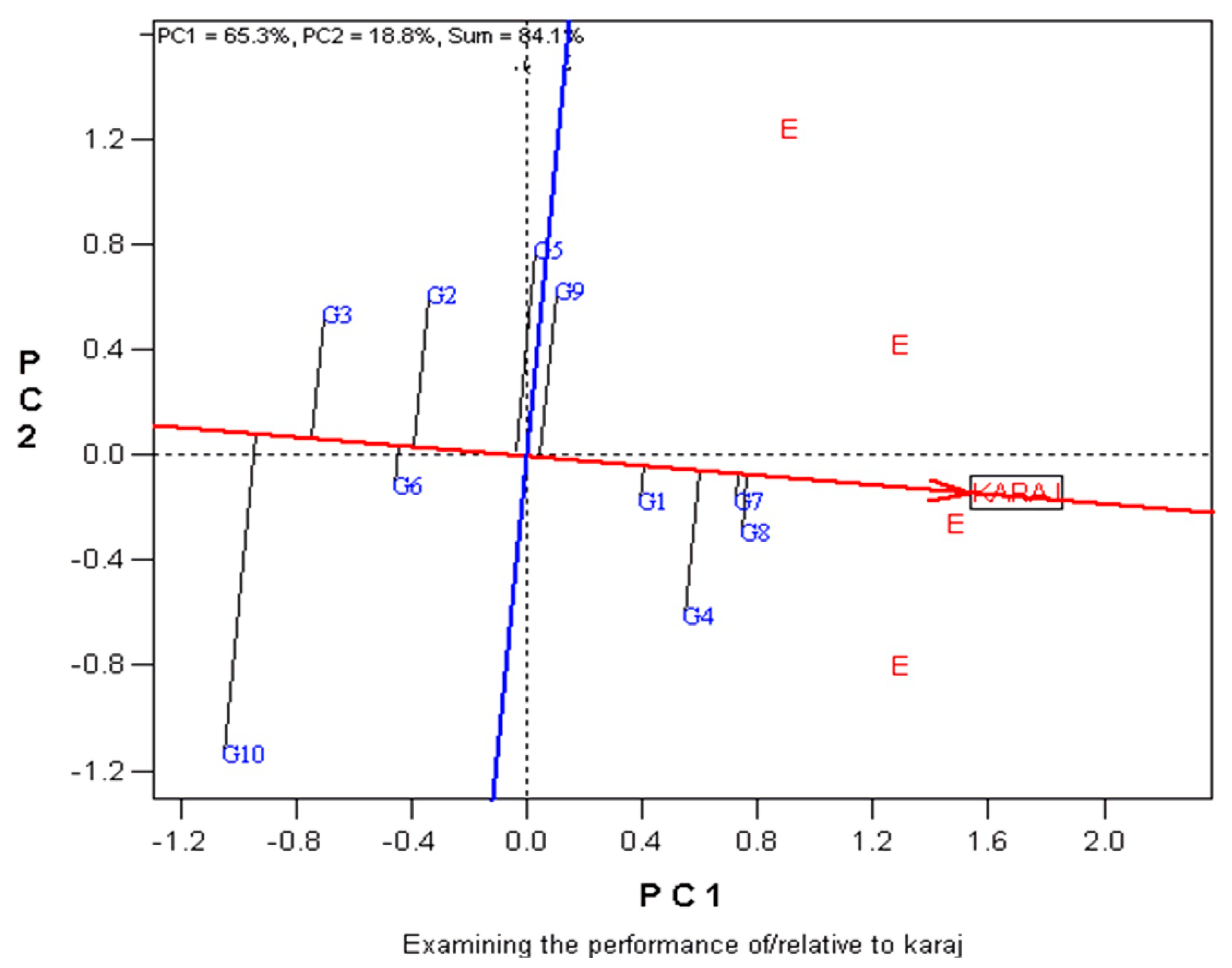
3.6. Ranking of Genotypes Based on the Most Suitable Environment (Karaj)
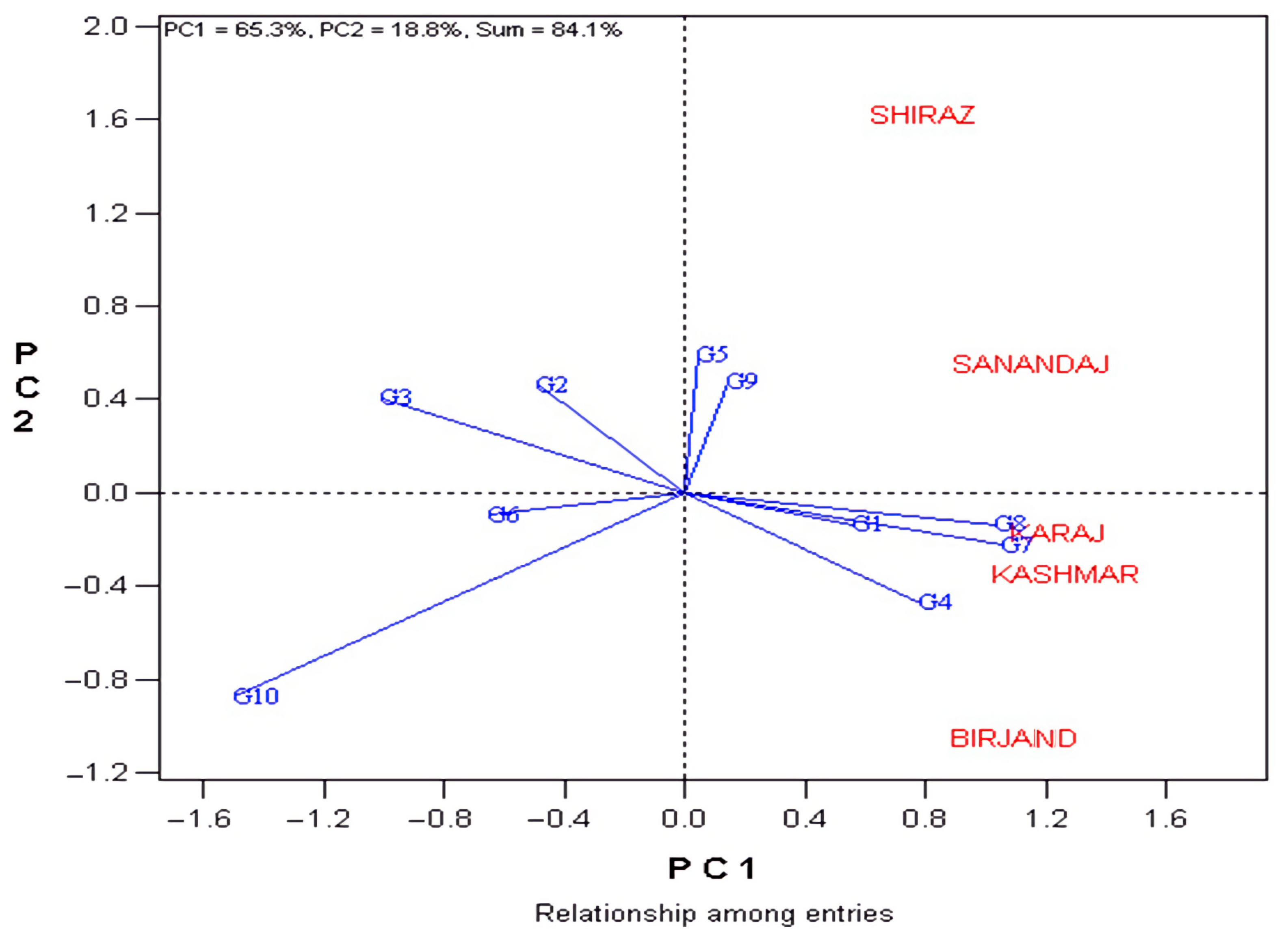
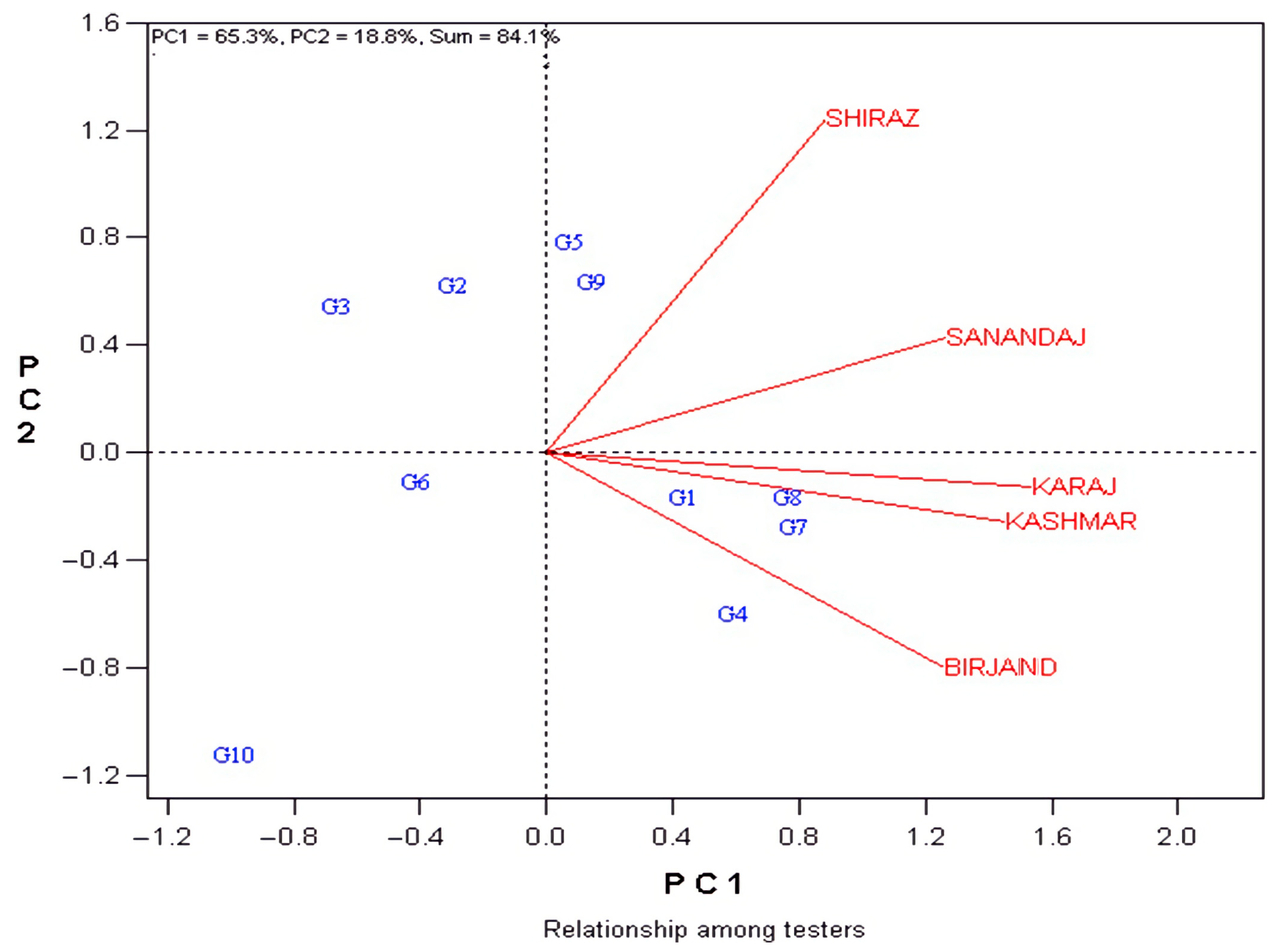
3.7. Relationships between Environments
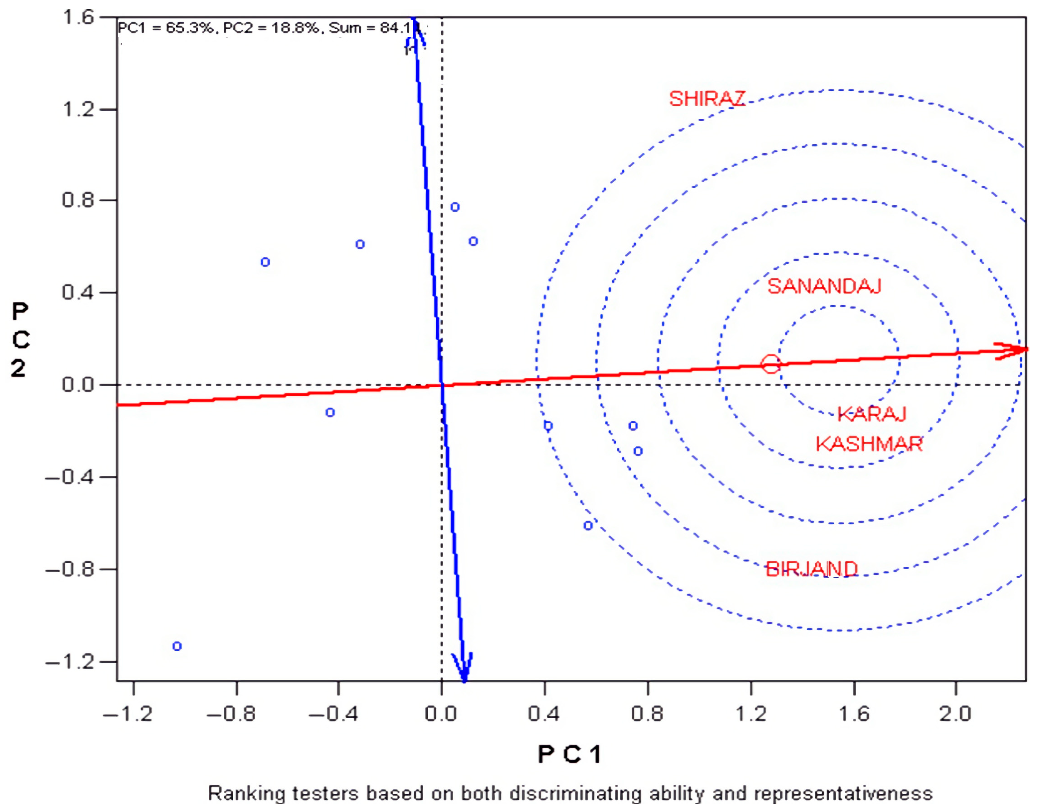
3.8. Ideal Environment with the Ranking Biplot
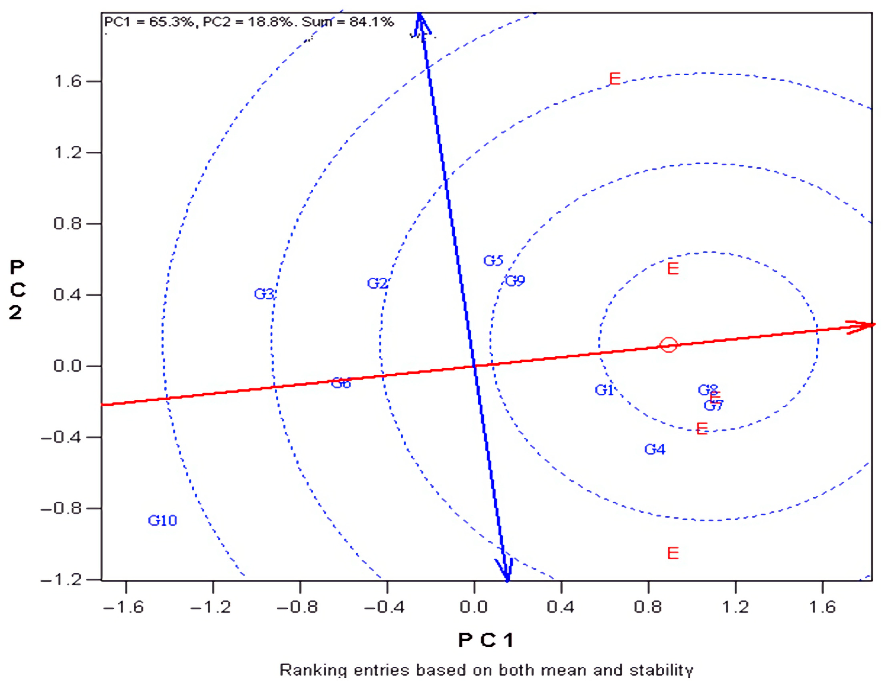
3.9. Ideal Genotype Based on Grain Yield and Stability Simultaneously
- (1)
- It has the highest yield of the entire dataset.
- (2)
- It is stable, as indicated by being located on the AEC abscissa.
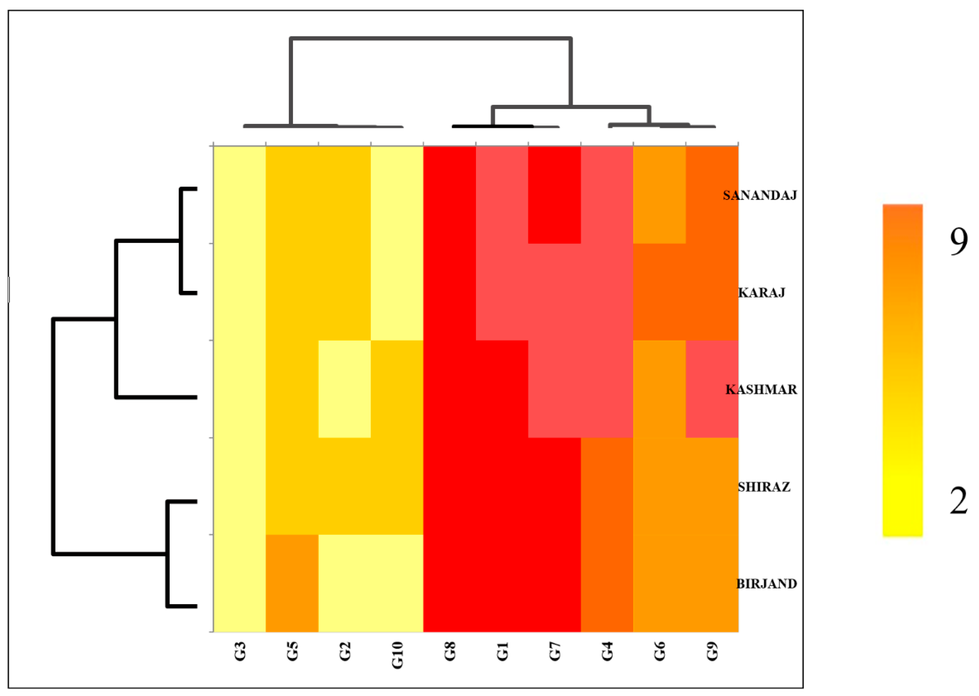
3.10. Cluster Analysis by Heat Map Method
4. Conclusions
Author Contributions
Funding
Institutional Review Board Statement
Informed Consent Statement
Data Availability Statement
Conflicts of Interest
References
- Eckes, A.H.; Gubała, T.; Nowakowski, P.; Szymczyszyn, T.; Wells, R.; Irwin, J.A.; Horro, C.; Hancock, J.M.; King, G.; Dyer, S.C.; et al. Introducing the Brassica Information Portal: Towards integrating genotypic and phenotypic Brassica crop data. F1000Research 2017, 6, 465. [Google Scholar] [CrossRef] [PubMed] [Green Version]
- Mohammadi, R.; Amri, A. Genotype × environment interaction implication: A case study of durum wheat breeding in Iran. In Advances in Plant Breeding Strategies: Agronomic, Abiotic and Biotic Stress Traits; Springer: Cham, Switzerland, 2016; pp. 515–558. [Google Scholar]
- Amiri, O.H.; Alem, Z.K.M.; Javidfar, F. Stability of seed yield in spring rapeseed (Brassica napus) genotypies. Iran. J. Crop Sci. 2004, 6, 203–2014. [Google Scholar]
- Rameeh, V. Combining ability and factor analysis in F2 diallel crosses of rapeseed varieties. Plant Breed. Seed Sci. 2001, 62, 73. [Google Scholar] [CrossRef]
- Klomsa-Ard, P.; Jaisil, P.; Patanothai, A. Performance and stability for yield and component traits of elite sugarcane genotypes across production environments in Thailand. Sugar Tech 2013, 15, 354–364. [Google Scholar] [CrossRef]
- Gauch, H.G., Jr. Statistical analysis of yield trials by AMMI and GGE. Crop Sci. 2004, 46, 1488–1500. [Google Scholar] [CrossRef]
- Muller, M.H.; Delieux, F.; Fernandez-Martinez, J.M.; Garric, B.; Lecomte, V.; Anglade, G.; Leflon, M.; Motard, C.; Segura, R. Occurrence, distribution and distinctive morphological traits of weedy Helianthus annuus L. populations in Spain and France. Genet. Resour. Crop Evol. 2009, 56, 869–877. [Google Scholar] [CrossRef]
- Karimizadeh, R.; Mohammadi, M.; Sabaghnia, N.; Shefazadeh, M.K. Using Huehn’s nonparametric stability statistics to investigate genotype× environment interaction. Not. Bot. Horti Agrobot. Cluj-Napoca 2012, 40, 293–301. [Google Scholar] [CrossRef] [Green Version]
- Yan, W.; Hunt, L.A.; Sheng, Q.; Szlavnics, Z. Cultivar evaluation and mega-environment investigation based on the GGE biplot. Crop Sci. 2000, 40, 597–605. [Google Scholar] [CrossRef]
- Makumbi, D.; Diallo, A.; Kanampiu, F.; Mugo, S.; Karaya, H. Agronomic performance and genotype× environment interaction of herbicide-resistant maize varieties in eastern Africa. Crop Sci. 2015, 55, 540–555. [Google Scholar] [CrossRef] [Green Version]
- Escobar, M.; Berti, M.; Matus, I.; Tapia, M.; Johnson, B. Genotype× environment interaction in canola (Brassica napus L.) seed yield in Chile. Chil. J. Agric. Res. 2011, 71, 175. [Google Scholar] [CrossRef] [Green Version]
- Nowosad, K.; Liersch, A.; Popławska, W.; Bocianowski, J. Genotype by environment interaction for seed yield in rapeseed (Brassica napus L.) using additive main effects and multiplicative interaction model. Euphytica 2016, 208, 187–194. [Google Scholar] [CrossRef] [Green Version]
- Mousavi, S.N.; Bodnár, K.; Nagy, J. Evaluation of decreasing moisture content of different maize genotypes. Acta Agrar. Debr. 2018, 30, 147–151. [Google Scholar] [CrossRef] [PubMed]
- Farshadfar, E.; Mohammadi, R.; Aghaee, M.; Vaisi, Z. GGE biplot analysis of genotype × environment interaction in wheat-barley disomic addition lines. Aust. J. Crop Sci. 2012, 6, 1074–1079. [Google Scholar]
- Yan, W.; Kang, M.S.; Ma, B.; Woods, S.; Cornelius, P.L. GGE biplot vs. AMMI analysis of genotype-by-environment data. Crop Sci. 2007, 47, 643–653. [Google Scholar] [CrossRef] [Green Version]
- Yan, W. Singular-value partitioning in biplot analysis of multienvironment trial data. Agron. J. 2002, 94, 990–996. [Google Scholar]
- Rahnejat, S.S.; Farshadfar, E. Evaluation of phenotypic stability in canola (Brassica napus) using GGE-biplot. Int. J. Biosci. 2015, 6, 350–356. [Google Scholar]
- Alizadeh, B.; Rezaizad, A.; Hamedani, M.Y.; Shiresmaeili, G.; Nasserghadimi, F.; Khademhamzeh, H.R.; Gholizadeh, A. Genotype× environment interactions and simultaneous selection for high seed yield and stability in Winter Rapeseed (Brassica napus) multi-environment trials. Agric. Res. 2022, 11, 185–196. [Google Scholar] [CrossRef]
- Mousavi, S.M.N.; Hejazi, P.; Khalkhali, S.K.Z. Study on stability of grain yield sunflower cultivars by AMMI and GGE biplot in Iran. Mol. Plant Breed. 2016, 7, 1–6. [Google Scholar]
- Yan, W. GGEbiplot—A Windows application for graphical analysis of multienvironment trial data and other types of two-way data. Agron. J. 2001, 93, 1111–1118. [Google Scholar] [CrossRef] [Green Version]
- Ansarifard, I.; Mostafavi, K.; Khosroshahli, M.; Reza Bihamta, M.; Ramshini, H. A study on genotype–environment interaction based on GGE biplot graphical method in sunflower genotypes (Helianthus annuus L.). Food Sci. Nutr. 2020, 8, 3327–3334. [Google Scholar] [CrossRef]
- Brar, K.S.; Singh, P.; Mittal, V.P.; Singh, P.; Jakhar, M.L.; Yadav, Y.; Sharma, M.M.; Shekhawat, U.S.; Kumar, C. GGE biplot analysis for visualization of mean performance and stability for seed yield in taramira at diverse locations in India. J. Oilseed Brassica 2016, 1, 66–74. [Google Scholar]
- Zhao, X.; Xia, H.; Wang, X.; Wang, C.; Liang, D.; Li, K.; Liu, G. Variance and stability analyses of growth characters in half-sib Betula platyphylla families at three different sites in China. Euphytica 2016, 208, 173–186. [Google Scholar] [CrossRef]
- D’Andrea, K.E.; Otegui, M.E.; Cirilo, A.G.; Eyherabide, G. Crop Physiology & Metabolism-Genotypic Variability in Morphological and Physiological Traits among Maize Inbred Lines—Nitrogen Responses. Crop Sci. 2006, 46, 1266–1276. [Google Scholar]
- Yan WeiKai, Y.W.; Hunt, L.A. Biplot analysis of multi-environment trial data. In Quantitative Genetics, Genomics and Plant Breeding; CABI Publishing: Wallingford, UK, 2002; pp. 289–303. [Google Scholar]
- Gunasekera, C.P.; Martin, L.D.; Siddique, K.H.M.; Walton, G.H. Genotype by environment interactions of Indian mustard (Brassica juncea L.) and canola (B. napus L.) in Mediterranean-type environments: 1. Crop growth and seed yield. Eur. J. Agron. 2006, 25, 1–12. [Google Scholar] [CrossRef]
- Yan, W.; Cornelius, P.L.; Crossa, J.; Hunt, L.A. Two types of GGE biplots for analyzing multi-environment trial data. Crop Sci. 2001, 41, 656–663. [Google Scholar] [CrossRef] [Green Version]
- Zhang, H.; Berger, J.D.; Milroy, S.P. Genotype× environment interaction studies highlight the role of phenology in specific adaptation of canola (Brassica napus) to contrasting Mediterranean climates. Field Crops Res. 2013, 144, 77–88. [Google Scholar] [CrossRef]
- Yan, W.; Rajcan, I. Biplot analysis of test sites and trait relations of soybean in Ontario. Crop Sci. 2002, 42, 11–20. [Google Scholar] [CrossRef]
- Thomason, W.E.; Phillips, S.B. Methods to evaluate wheat cultivar testing environments and improve cultivar selection protocols. Field Crops Res. 2006, 99, 87–95. [Google Scholar] [CrossRef]
- Navabi, A.; Yang, R.C.; Helm, J.; Spaner, D.M. Can spring wheat-growing megaenvironments in the northern Great Plains be dissected for representative locations or niche-adapted genotypes? Crop Sci. 2006, 46, 1107–1116. [Google Scholar] [CrossRef]
- Yan, W.; Wu, H.X. Application of GGE biplot analysis to evaluate genotype (G), environment (E), and G× E interaction on Pinus radiata: A case study. N. Z. J. For. Sci. 2008, 38, 132–142. [Google Scholar]
- Yan, W.; Tinker, N.A. Biplot analysis of multi-environment trial data: Principles and applications. Can. J. Plant Sci. 2006, 86, 623–645. [Google Scholar] [CrossRef] [Green Version]
- Roy, D. Plant Breeding Analysis and Exploitation of Variation; Alpha Science International Ltd.: London, UK, 2000. [Google Scholar]
- Yan, W.; Holland, J.B. A heritability-adjusted GGE biplot for test environment evaluation. Euphytica 2010, 171, 355–369. [Google Scholar] [CrossRef] [Green Version]
- Omrani, A.; Omrani, S.; Khodarahmi, M.; Shojaei, S.H.; Illés, Á.; Bojtor, C.; Mousavi, S.M.N.; Nagy, J. Evaluation of grain yield stability in some selected wheat genotypes using AMMI and GGE biplot methods. Agronomy 2022, 12, 1130. [Google Scholar] [CrossRef]
- Erdemci, I. Investigation of genotype× environment interaction in chickpea genotypes using AMMI and GGE biplot analysis. Turk. J. Field Crops 2018, 23, 20–26. [Google Scholar] [CrossRef] [Green Version]
- Meng, Y.; Ren, P.; Ma, X.; Li, B.; Bao, Q.; Zhang, H.; Wang, J.; Bai, J.; Wang, H. GGE biplot-based evaluation of yield performance of barley genotypes across different environments in China. J. Agric. Sci. Technol. 2016, 18, 533–543. [Google Scholar]


| Genotype No. | Genotype | Origin | Genotype No. | Genotype | Origin |
|---|---|---|---|---|---|
| G1 | Sarigol | Iran | G6 | Likord | Germany |
| G2 | Hyola308 | Canada | G7 | Okapi | France |
| G3 | Option500 | Germany | G8 | Hyola401 | Canada |
| G4 | Opera | Sweden | G9 | Zarfam | Iran |
| G5 | Modena | Denmark | G10 | Modena | Denmark |
| Area | Longitude | Latitude | Elevation AMSL (m) | Temperature (°C) | Rainfall Average (2016–2017) | EC(ds/m) | Acidity | Lime (%) | Organic Carbon (%) | Organic Materials (%) | Clay (%) | Silt (%) | Sand (%) |
|---|---|---|---|---|---|---|---|---|---|---|---|---|---|
| Karaj | 50°54′ E | 35°55′ N | 1312 | 18.3 | 288.5 | 0.20 | 8.2 | 7 | 32 | 45 | 32 | 25 | 22 |
| Birjand | 59°12′ E | 32°52′ N | 1491 | 21 | 143.95 | 0.5 | 7.4 | 8 | 25 | 35 | 42 | 18 | 31 |
| Shiraz | 52°36′ E | 29°32′ N | 1484 | 17 | 328.9 | 0.26 | 7.22 | 6 | 42 | 53 | 34 | 28 | 16 |
| Kashmar | 58°48′ E | 35°53′ N | 1109 | 19 | 198 | 0.32 | 7.88 | 7 | 36 | 51 | 31 | 24 | 24 |
| Sanandaj | 47°00′ E | 35°20′ N | 1373 | 16 | 461 | 0.27 | 7.45 | 7 | 40 | 46 | 36 | 22 | 24 |
| Source of Variation | df | Sum of Squares | Mean Square | % of L + G + GL | % of Y + G + GY | p Value |
|---|---|---|---|---|---|---|
| Location (L) | 4 | 212.50 | 53.12 ** | 68.44 | p < 0.001 | |
| Year (Y) | 1 | 0.78 | 0.78 ** | 8.69 | p < 0.001 | |
| Location × Year (L × Y) | 4 | 277.55 | 0.69 ** | p < 0.001 | ||
| Rep/(Loc × Year) | 20 | 11.55 | 0.57 | |||
| Genotype (G) | 9 | 57.87 | 6.43 ** | 18.63 | 58.60 | p < 0.001 |
| Location × Genotype (L × G) | 36 | 40.08 | 1.11 ** | 12.91 | p < 0.001 | |
| Year × Genotype (Y × G) | 9 | 32.28 | 3.58 ** | 32.69 | p < 0.001 | |
| Location× Year × Genotype | 36 | 137.74 | 3.82 ** | p < 0.001 | ||
| Error | 299 | 140.39 | 53.12 |
Disclaimer/Publisher’s Note: The statements, opinions and data contained in all publications are solely those of the individual author(s) and contributor(s) and not of MDPI and/or the editor(s). MDPI and/or the editor(s) disclaim responsibility for any injury to people or property resulting from any ideas, methods, instructions or products referred to in the content. |
© 2023 by the authors. Licensee MDPI, Basel, Switzerland. This article is an open access article distributed under the terms and conditions of the Creative Commons Attribution (CC BY) license (https://creativecommons.org/licenses/by/4.0/).
Share and Cite
Shojaei, S.H.; Mostafavi, K.; Ghasemi, S.H.; Bihamta, M.R.; Illés, Á.; Bojtor, C.; Nagy, J.; Harsányi, E.; Vad, A.; Széles, A.; et al. Sustainability on Different Canola (Brassica napus L.) Cultivars by GGE Biplot Graphical Technique in Multi-Environment. Sustainability 2023, 15, 8945. https://doi.org/10.3390/su15118945
Shojaei SH, Mostafavi K, Ghasemi SH, Bihamta MR, Illés Á, Bojtor C, Nagy J, Harsányi E, Vad A, Széles A, et al. Sustainability on Different Canola (Brassica napus L.) Cultivars by GGE Biplot Graphical Technique in Multi-Environment. Sustainability. 2023; 15(11):8945. https://doi.org/10.3390/su15118945
Chicago/Turabian StyleShojaei, Seyed Habib, Khodadad Mostafavi, Seyed Hamed Ghasemi, Mohammad Reza Bihamta, Árpád Illés, Csaba Bojtor, János Nagy, Endre Harsányi, Attila Vad, Adrienn Széles, and et al. 2023. "Sustainability on Different Canola (Brassica napus L.) Cultivars by GGE Biplot Graphical Technique in Multi-Environment" Sustainability 15, no. 11: 8945. https://doi.org/10.3390/su15118945