Marginal Carbon Dioxide Emission Reduction Cost and Influencing Factors in Chinese Industry Based on Bayes Bootstrap

Abstract

Accurate measurement of the shadow price of carbon dioxide (CO₂) is fundamental to the scientific assessment of the carbon emission reduction cost and the formulation and execution of China’s carbon emission mitigation policies. Underpinned by the directional distance function, this research uses a parametric linear programming method and a Bayes bootstrap estimation method to estimate the marginal CO₂ emission reduction cost of the industrial sector in China and to quantify the related influencing factors. The results revealed that the marginal reduction cost of industrial CO₂ is CNY 4565/ton. The marginal reduction cost of CO₂ varies by industry, with the textile industry being the highest and the petroleum, coking and nuclear fuel processing industries the lowest. Meanwhile, an increasing number of industries are shifting to cleaner production. Furthermore, the marginal reduction cost of industrial CO₂ has an “inverted U-shaped” relation with carbon intensity. Carbon emission reduction can be accomplished effectively if the carbon intensity is kept below the threshold value of 0.41 tons/CNY 10,000.

1. Introduction

At present, the global climate catastrophe is becoming increasingly severe. Accelerating carbon emission reduction to combat global warming has become the mainstream consensus worldwide. Being the world’s top emitter of carbon dioxide (CO₂), China has taken the initiative to shoulder international responsibilities commensurate with its own level of development. Over the years, China has been committed to promoting and implementing global carbon reduction work and has made outstanding contributions to addressing the Paris Agreement on climate change and resolving complex problems in international relations. In 2009, China announced its quantified carbon emission reduction targets at the Copenhagen Climate Conference, pledging to reduce CO₂ emissions per unit of GDP (i.e., carbon emission intensity) by 40% to 45% from its previous level in 2005 by 2020. In 2015, China subscribed to an Intended Nationally Determined Contribution to tackle climate change. At the Paris Climate Summit, China renewed its commitment to curb CO₂ emission intensity by 60% to 65% from 2005 levels by 2030 and to achieve carbon peaking by around 2030. In 2020, President Xi further proclaimed the carbon emission reduction target at the Climate Ambition Summit. By 2030, China will have reduced its CO₂ emission intensity by more than 65% compared to the level in 2005. While setting carbon emission reduction targets and goals, the Chinese government is also actively exploring market-based policy instruments to drive carbon emission reduction. A pilot environmental tax was introduced back in the 1990s. Since 2011, pilot regional carbon emission trading has been launched in seven cities and provinces, covering Beijing, Shanghai and Guangdong. The national carbon emission trading was officially initiated in July 2021.

Currently, carbon taxes and carbon emission trading are two of the most important market-based policy instruments at home and abroad [1]. Both approaches to controlling carbon emissions have their pros and cons, according to the government and academic debate. The effectiveness of policy implementation is closely related to the development of each country, as well as the status and potential for emission reductions in different sectors within the country. At present, China’s regional economic development is uneven, with widely varying industrial structures [2]. On the one hand, different regions and industries have different priorities in facilitating carbon emission reduction [3]. On the other hand, the efficiency, potential and cost of carbon reduction vary considerably between districts and sectors [4]. It is therefore crucial to accurately measure the shadow price of CO₂.

Accurate measurement of the shadow price of CO₂ is the basic work to scientifically evaluate China’s current carbon emission reduction potential and costs. It can not only provide references for the initial trading price of the carbon emission rights market but also furnish theoretical support and practical guidance for the government to formulate a reasonable carbon tax policy [5]. In this paper, we reviewed the relevant literature [6,7,8] on shadow price measurement models for CO₂ and discovered that most scholars rarely addressed the impact of stochastic perturbation factors on undesirable output when choosing Parametric Linear Programming (PLP) to gauge the shadow price of CO₂. At the same time, they did not validly test the estimates, resulting in a discrepancy between the measured shadow price of CO₂ and the real one. Hence, this paper focuses on how to reduce uncertainty in the measurement of the shadow price of CO₂ and improve the scientific validity of the shadow price of CO₂.

The contribution of this paper is as follows: (1) It attempts to construct a robust estimation method by introducing an effective statistical error tool, Bayes bootstrap, to improve and optimize the model for measuring the shadow price of CO₂. (2) It analyzes in detail the shadow price of industrial CO₂ in terms of time trends and industry differences. (3) It constructs a panel regression model to relate carbon intensity and marginal emission reduction costs and to further fit industrial marginal emission reduction cost curves.

This article is structured as follows: Section 2 presents a review of the available relevant literature; Section 3 constructs a theoretical model of the shadow price of CO₂ and presents its estimation approach; Section 4 describes the relevant variables and data; Section 5 analyzes and addresses the empirical data; Section 6 gives the research conclusion.

2. Literature Review

Over the last few years, numerous studies have been undertaken by domestic and international scholars on the popular issue of CO₂ reduction costs. According to the existing literature, the models adopted to assess the cost of CO₂ emission reduction mainly include the bottom-up model, the top-down model, the hybrid model, and the efficiency analysis model. Among them, the bottom-up model comprises the engineering economic model [9] and the dynamic optimization model [10]. It focuses on analyzing the technical details of carbon emission reduction and is primarily used to analyze the carbon emission reduction costs of various technology options. However, it ignores the impact of carbon emission reduction in the energy sector on other industries and the macroeconomy [11,12]. In contrast, the top-down model includes the macroeconomic model [13], the input-output model [14] and the computable general equilibrium (CGE) model [15], etc. The advantage of this type of model lies in its ability to simulate the relationship between the energy industry and other industries. Meanwhile, it can provide insight into the influence of carbon emission reduction policies on industrial sectors and the macroeconomy. Nonetheless, it lacks a specific description of carbon emission reduction technologies. In parallel, the hybrid model, combining the advantages of bottom-up and top-down models, can analyze the cost of carbon emission reduction from technical and economic perspectives. However, its construction and calculation process is particularly complicated due to the high degree of aggregation [16]. The last type of model, namely, the efficiency analysis model [17], is based on the microscopic production theory. By modeling the production technology containing CO₂ emissions, the resulting shadow price represents the trade-off between good and bad output, which is considered the marginal emission reduction cost [18]. The efficiency analysis model allows for a more direct assessment of the cost of CO₂ emission reduction than the other three models mentioned above. In addition, it is more popular among scholars because of its relaxed requirements on sample data and simple calculation process.

Depending on the methods used to construct the production frontier, the efficiency analysis model is subdivided into parametric and non-parametric models. Non-parametric methods are mainly based on data envelopment analysis (DEA), which has the advantage of not requiring a pre-determined functional form and being more flexible in estimating the shadow price of CO₂ [17,19,20,21,22,23]. However, the piecewise function adopted by non-parametric methods in constructing the production frontier cannot guarantee the differentiability of all positions. In addition, non-parametric methods are susceptible to outliers, leading to non-unique estimates [24]. In contrast to non-parametric methods, parametric methods can set differentiable production boundary functions in advance to ensure the uniqueness of estimation results [25]. Therefore, parametric models are more suitable than non-parametric models for estimating the shadow price of CO₂.

According to the form of the function, parameter methods can be divided into the distance function and the directional distance function. The former requires that good outputs and bad outputs vary proportionally. In contrast, the latter allows for the parallel observation of an augmentation of good outputs and a reduction of bad outputs, which is consistent with the carbon emission reduction goals pursued by enterprises and is widely used to estimate marginal emission reduction costs. According to the differences in methods, parametric methods are further divided into the parametric linear programming method [26,27,28,29] and the stochastic frontier analysis method [30,31,32,33,34]. Both methods have their pros and cons. In particular, the advantage of the stochastic frontier analysis method is that it accounts for statistical noise. Nonetheless, it cannot incorporate constraints into the analysis and inevitably encounters endogeneity problems when obtaining production function [35]. In contrast, the parametric linear programming method in the estimation process, albeit able to impose the constraints assumed by the directional distance function, is unable to deal with the influence of random disturbance factors on the shadow price of bad output or to effectively test the estimates. This results in a certain deviation of the measured results from the actual results, which can be remedied through bootstrap simulation [36].

Throughout the literature above, each of the four types of models has advantages and disadvantages, but the efficiency analysis model based on the directional distance function is superior in evaluating the shadow price of CO₂. Therefore, this paper applies the efficiency analysis model of the directional distance function and adopts the parametric linear programming method. Meanwhile, a more optimized Bayes bootstrap estimation method was introduced to obtain a more robust shadow price of CO₂ by correcting the deviation of the original parameters so as to make up for the shortcomings of the parametric linear programming method.

3. Research Methods

3.1. Research Framework

With the directional distance function as a basis, this research uses a parametric linear programming method and a Bayes bootstrap estimation method to gauge the marginal emission reduction cost of industrial CO₂ in China. On this basis, the influential factors of marginal emission reduction costs are further studied through an econometric model. Figure 1 shows the research framework of this article.

3.2. Directional Distance Function

In this paper, the setting of Färe et al. [25] is followed, and it is assumed that $N$ input factors $x=\left(x_1,x_2,\cdots ,x_N\right)\in R_{+}^N$ are used in the production process to produce $M$ good outputs $y=\left(y_1,y_2,\cdots ,y_M\right)\in R_{+}^M$ and $L$ bad outputs $b=\left(b_1,b_2,\cdots ,b_L\right)\in R_{+}^L$. The production technology in the production process can be specified as the following output sets:

$$P\left(x\right)=\left\{\left(y,b\right):x can produce\left(y,b\right)\right\}$$

(1)

The output set $P\left(x\right)$ needs to satisfy the standard production theory assumptions [18]: compactness and free disposal of inputs. In this context, the compactness assumption implies that finite inputs cannot be produced indefinitely, while the input disposability assumption means that output will not decrease unless inputs are reduced. In addition, $P\left(x\right)$ also satisfies weak disposability and null hypothesis and can be denoted as follows:

(i)

If $\left(y,b\right)\in P\left(x\right)$, and $0\le \theta \le 1$, then $\left(\theta y,\theta b\right)\in P\left(x\right)$

(ii)

If $\left(y,b\right)\in P\left(x\right)$, and $b=0$, then $y=0$

The weak disposability assumption (i) states that any good and bad outputs are proportional, implying that any reduction in bad outputs has a cost, whereas the null hypothesis (ii) implies that as long as there is a good output in production, there must be a bad output, and the only way to avoid bad output is to stop all production.

Under the constraints of the above assumptions, this essay further employs a directional distance function to represent the production technology. Given that the direction vector $g=\left(g_y,g_b\right)\in R_{+}^M\times R_{+}^L$, and $g\ne 0$, the directional distance function can be stated as:

$$\overrightarrow{D}\left(x,y,b;g_y,g_b\right)=max\left\{\beta :\left(y+\beta g_y,b-\beta g_b\right)\in P\left(x\right)\right\}$$

(2)

The directional distance function delineates the maximum feasible increment of good output and the maximum feasible decrement of bad output under a given production technique $P\left(x\right)$. The process is depicted in Figure 2. Given production technology $P\left(x\right)$ and direction vector $g=\left(g_y,g_b\right)>0$, the bad output ${\beta }^{*}{g}_b$ is reduced, while the good output ${\beta }^{*}{g}_y$ is expanded along the direction vector until it reaches point $B\left(y+{\beta }^{*}{g}_y,b-{\beta }^{*}{g}_b\right)$ on the boundary of production set $P\left(x\right)$. ${\beta }^{*}=\overrightarrow{D}\left(x,y,b;g_y,-g_b\right)$ is the specific value of the directional distance function. The directional distance function is an efficiency index, and $\beta$ is the inefficiency value, representing the optimal expansion or reduction degree. The larger the $\beta$ value is, the lower the technical efficiency is. If $\beta =0$, the production technology is effective and at the forefront of production.

Since the directional distance function is established based on the production set $P\left(x\right)$, it also satisfies the basic properties of $P\left(x\right)$, which are elaborated as follows by Färe et al. [25]:

(i)

If and only if $\left(y,b\right)\in P\left(x\right)$, then $\overrightarrow{D}\left(x,y,b;g_y,-g_b\right)\ge 0$

(ii)

If $\left(y^{\prime },b\right)\le y,b\in P\left(x\right)$, then $\overrightarrow{D}\left(x,y^{\prime },b;g_y,-g_b\right)\ge \overrightarrow{D}\left(x,y,b;g_y,-g_b\right)$

(iii)

If $\left(y,b^{\prime }\right)\ge y,b\in P\left(x\right)$, then $\overrightarrow{D}\left(x,y,b^{\prime };g_y,-g_b\right)\ge \overrightarrow{D}\left(x,y,b;g_y,-g_b\right)$

(iv)

If $\left(y,b\right)\in P\left(x\right) and 0\le \theta \le 1$, then $\overrightarrow{D}\left(x,\theta y,\theta b;g_y,-g_b\right)\ge 0$

Property (i) states that for any viable production vector, the directional distance function has a non-negative value. Property (ii) indicates that the bad output remains constant under a given input, whereas the value of the directional distance function does not grow accordingly as good output increases. Property (iii) denotes that the good output remains unchanged under a given input, and the value of the directional distance function does not decline even if the bad output increases. Property (iv) demonstrates that the good and bad outputs satisfy weak disposability. In addition, the directional distance function meets the transformation property:

$$\overrightarrow{D}\left(x,y+\alpha g_y,b-\alpha g_b;g_y,-g_b\right)=\overrightarrow{D}\left(x,y,b;g_y,-g_b\right)-\alpha$$

(3)

where $\alpha$ is a scalar. The transformation property shows that if the good output increases $\alpha g_y$ while the bad output decreases $\alpha g_b$, then the value of the directional distance function will decrease $\alpha$ accordingly.

3.3. Shadow Price of Bad Output

To find the shadow price of undesirable output, the dual property between the directional distance function and the yield function should be utilized. Therefore, the income function is constructed, and the good output price vector is specified as $p=\left(p_1,p_2,\cdots ,p_M\right)\in R_{+}^M$ and the bad output price vector is determined as $q=\left(q_1,q_2,\cdots ,q_L\right)\in R_{+}^L$, following the method of Färe et al. [25]. The existence of bad output is assumed to lead to a reduction in income, and the income function is set as follows:

$$R\left(x,p,q\right)=max\left\{py-qb:\left(y,b\right)\in P\left(x\right)\right\}$$

(4)

Using the property (i) of the directional distance function, the following income function can be attained:

$$R\left(x,p,q\right)=max\left\{py-qb:\overrightarrow{D}\left(x,y,b;g\right)\ge 0\right\}$$

(5)

The income function describes the maximum feasible income that the observed subject can obtain when facing the good output price $p$ and the bad output price $q$. If $y,b\in P\left(x\right)$, there must be $(y+\beta g_y,b-\beta g_b)\in P\left(x\right)$. Therefore, given a feasible direction vector $g=(g_y,g_b)$, the following results can be obtained:

$$R\left(x,p,q\right)\ge \left(py-qb\right)+p\overrightarrow{D}\left(x,y,b;g\right)g_y+q\overrightarrow{D}\left(x,y,b;g\right)g_b$$

(6)

The left-hand side of Equation (6) signifies the maximum achievable return, and the right-hand side corresponds to the observed return plus the return obtained by increasing the good output along $g_y$ and the return obtained by decreasing the bad output along $g_b$.

After rearranging Equation (6), the following Equation can be obtained:

$$\overrightarrow{D}\left(x,y,b;g\right)\le \frac{R(x,p,q)-\left(py-qb\right)}{p{g}_y+q{g}_b}$$

(7)

Thus, the directional distance function can be obtained by the yield function:

$$\overrightarrow{D}\left(x,y,b;g\right)=min\left\{\frac{R\left(x,p,q\right)-\left(py-qb\right)}{p{g}_y+q{g}_b}\right\}$$

(8)

Based on the data envelope theorem, the two first-order terms can be obtained as follows:

$${\nabla }_y\overrightarrow{D}\left(x,y,b;g\right)=\frac{-p}{p{g}_y+q{g}_b}\le 0$$

(9)

$${\nabla }_b\overrightarrow{D}\left(x,y,b;g\right)=\frac{q}{p{g}_y+q{g}_b}\ge 0$$

(10)

Shadow prices for bad output can be obtained by sorting:

$$q_j=-p_m\left(\frac{\partial \overrightarrow{D}\left(x,y,b;g\right)/\partial b_j}{\partial \overrightarrow{D}\left(x,y,b;g\right)/\partial y_m}\right)$$

(11)

where $\frac{\partial \overrightarrow{D}/\partial b}{\partial \overrightarrow{D}/\partial y}$ is the slope of the tangent line of the observation object $\left(y,b\right)$ on the boundary of the production set $P\left(x\right)$, namely, the marginal conversion rate of good output and bad output on the boundary of the production set $P\left(x\right)$. This indicates the decrease in good output when reducing one unit of undesirable output, which is multiplied by the price of the good output to give a shadow price $q$. The shadow price $q$ represents the opportunity cost of cutting one unit of bad output, i.e., the marginal abatement cost of reducing emissions.

3.4. The Parametric Linear Programming Model

The directional distance function can be categorized as the translog function and the quadratic function. As the quadratic function satisfies the conversion property of the directional distance function and has first- and second-order parameters for calculating marginal effects [37,38,39], it is adopted in this paper for parameter estimation. This paper follows the setting of Färe et al. [25] and sets the direction vector to $g=\left(g_y,g_b\right)=\left(1,1\right)$, indicating that good output expands while bad output shrinks in the same range.

Assuming that there are $k=1,2,\dots ,K$ decision units and production is carried out in year $t=1,2,\dots ,T$, then the quadratic directional distance function of the $k$ decision unit in year $t$ can be expressed as:

$$\begin{gathered} \overrightarrow{D_0}\left(x^t{}_k,y^t{}_k,b^t{}_k;1,-1\right)=\alpha +\sum _{n=1}^N{\alpha }_n{x}^t{}_{nk}+\sum _{m=1}^M{\beta }_m{y}^t{}_{mk}+\sum _{l=1}^L{\gamma }_l{b}^t{}_{lk}+\frac{1}{2}\sum _{n=1}^N\sum _{n^{\prime }=1}^N{\alpha }_{n{n}^{\prime }}{x}^t{}_{nk}{x}^t{}_{n^{\prime }k} \\ +\frac{1}{2}\sum _{m=1}^M\sum _{m^{\prime }=1}^M{\beta }_{m{m}^{\prime }}{y}^t{}_{mk}{y}^t{}_{m^{\prime }k}+\frac{1}{2}\sum _{l=1}^L\sum _{l^{\prime }=1}^L{\gamma }_{l{l}^{\prime }}{b}^t{}_{lk}{b}^t{}_{l^{\prime }k}+\sum _{n=1}^N\sum _{m=1}^M{\delta }_{nm}{x}^t{}_{nk}{y}^t{}_{mk} \\ +\sum _{n=1}^N\sum _{l=1}^L{\eta }_{nl}{x}^t{}_{nk}{b}^t{}_{lk}+\sum _{m=1}^M\sum _{l=1}^L{\mu }_{ml}{y}^t{}_{mk}{b}^t{}_{lk} \end{gathered}$$

(12)

In order to control the individual effect and time effect, the individual dummy variable $I$ and time dummy variable $T$ are added to the intercept term of Equation (12), referring to Fare et al. [18]:

$$\alpha ={\alpha }_0+{\sum }_{k=1}^K{D}_{I_k}{I}_k+{\sum }_{t=1}^T{D}_{T_t}{T}_t$$

(13)

Under the above settings, the linear programming method is adopted in this paper to solve the parameters in Equation (12), which requires the objective function to be minimized through parameter selection [40]. Therefore, further constraints need to be set for unknown parameters:

$$\begin{gathered} min\sum _{t=1}^T\sum _{k=1}^K\left. [\overrightarrow{D_0}(x^t{}_k,y^t{}_k,b^t{}_k;g_y,g_b)-0\right] \\ \left(i\right) \overrightarrow{D_0}\left(x^t{}_k,y^t{}_k,b^t{}_k;g_y,g_b\right)\ge 0, k=1,2,\cdots \cdots ,K; t=1,2,\cdots \cdots ,T \\ \left(\mathrm{ii}\right) \frac{\partial \overrightarrow{D_0}\left(x^t{}_k,y^t{}_k,b^t{}_k;g_y,g_b\right)}{\partial b_l}\ge 0, l=1,2,\cdots \cdots ,L; k=1,2,\cdots \cdots ,K; t=1,2,\cdots \cdots ,T \\ \left(\mathrm{iii}\right) \frac{\partial \overrightarrow{D_0}\left(x^t{}_k,y^t{}_k,b^t{}_k;g_y,g_b\right)}{\partial y_m}\le 0, m=1,2,\cdots \cdots ,M; k=1,2,\cdots \cdots ,K; t=1,2,\cdots \cdots ,T \\ \left(\mathrm{iv}\right) \frac{\partial \overrightarrow{D_0}\left(x^t{}_k,y^t{}_k,b^t{}_k;g_y,g_b\right)}{\partial x_n}\ge 0, n=1,2,\cdots \cdots ,N; k=1,2,\cdots \cdots ,K; t=1,2,\cdots \cdots ,T \\ \left(v\right) {\alpha }_{n{n}^{\prime }}={\alpha }_{n^{\prime }n}, n\ne n^{\prime }; {\beta }_{m{m}^{\prime }}={\beta }_{m^{\prime }m},m\ne m^{\prime }; {\gamma }_{l{l}^{\prime }}={\gamma }_{l^{\prime }l},l\ne l^{\prime } \\ \left(\mathrm{vi}\right) {\sum }_{m=1}^M{\beta }_m-{\sum }_{l=1}^L{\gamma }_l=-1 \\ {\sum }_{m^{\prime }=1}^M{\beta }_{m{m}^{\prime }}-{\sum }_{l=1}^L{\mu }_{ml}=0, m=1,2,\cdots \cdots ,M \\ {\sum }_{l^{\prime }=1}^L{\gamma }_{l{l}^{\prime }}-{\sum }_{m=1}^M{\mu }_{ml}=0, l=1,2,\cdots \cdots ,L \\ {\sum }_{m=1}^M{\delta }_{nm}-{\sum }_{l=1}^L{\eta }_{nl}=0, n=1,2,\cdots \cdots ,N \end{gathered}$$

(14)

In Equation (14), constraint (i) requires that all observation points are feasible, that is, non-negative of the directional distance function. Constraints (ii), (iii) and (iv) impose monotone properties on all inputs and outputs, implying that an uplift in good outputs or a drop in bad outputs can reduce the distance between the observed object and the production frontier. The constraints (v) and (vi) correspond to the symmetry and conversion of the directional distance function, respectively.

3.5. Bayes Bootstrap

The advantage of parametric linear programming methods is that the constraints assumed by the directional distance function can be applied. Nevertheless, it has its own limitations in that it cannot deal with the influence of random disturbance factors on the shadow price of bad output, nor can it provide a valid test of the estimated results, which would greatly reduce the accuracy and effectiveness of the shadow price estimation of CO₂. To address the above issues, this paper introduces an effective Bayes bootstrap estimation method for statistical error and hypothesis testing. Robust estimates of the shadow price of CO₂ are obtained by iterative sampling and correction for bias due to sampling variation, which remedies the shortcomings of the linear programming method.

The specific steps are as follows:

(i)

The sample was assumed to be $X=\left(x_1,x_2,\cdots ,x_m\right)$, and each Bayes bootstrap resampled to the posterior probability generated by each $x_j$, $j=1,2,\cdots ,m$.

(ii)

A Bayes bootstrap sample was generated by $m-1$ random variables $u_1,u_2,\cdots ,u_{m-1}$ which obeyed (0,1) uniform distribution. The generated random variables were sorted from smallest to largest.

(iii)

The difference values $g_j=u_j-u_{j-1}$ were calculated, $j=1,2,\cdots ,m$, where $u_0=0$, $u_m=1$.

(iv)

The difference value $g=\left(g_1,g_2,\cdots ,g_m\right)$ was the probability vector attached to the data value $x_1,x_2,\cdots ,x_m$ in Bayes bootstrap resampling. Namely, $\sum _{j=1}^m{g}_j{x}_j$, $g_j$ obeyes Dirichlet distribution and satisfies the conditions of $\sum _{j=1}^m{g}_j=1$.

(v)

(i)–(iv) were repeated several times (1000 times in this paper) to obtain several Bayes bootstrap samples, which were then fitted to model (14) for parameter estimation, and the corresponding Bayes bootstrap sample estimation results were obtained.

(vi)

The revised parameter estimates and standard errors were calculated.

$$\tilde{q}=\widehat{q}-bias\left({\widehat{q}}^{*}\right)=\widehat{q}-\left(\overline{{\widehat{q}}^{*}}-\widehat{q}\right)=2\widehat{q}-\overline{{\widehat{q}}^{*}}$$

(15)

$$SE\left({\widehat{q}}^{*}\right)=\sqrt{\frac{1}{S-1}{\sum }_{s=1}^S{\left({\widehat{q}}^{*}{}_s-\overline{{\widehat{q}}^{*}}\right)}^2}$$

(16)

4. Variables and Data

Based on the directional distance function, this paper adopts the parametric linear programming method and the Bayes bootstrap estimation method to remove anomalous years and selects the shadow price of industrial CO₂ in China from 1998 to 2019. Due to the lack of data prior to 2003 for “other mining industries”, “other manufacturing industries” and “waste resource comprehensive utilization industries”, these three industries were excluded from the samples, following the practice of Li and Lin [41]. Therefore, 36 industrial sectors were finally selected as research objects in this paper, as presented in

Table 1. A list of industrial sectors.

Code	Industrial Sector	Code	Industrial Sector
ind01	Coal Mining and Dressing	ind19	Raw Chemical Materials and Chemical Products
ind02	Petroleum and Natural Gas Extraction	ind20	Medical and Pharmaceutical Products
ind03	Ferrous Metals Mining and Dressing	ind21	Chemical Fiber
ind04	Nonferrous Metals Mining and Dressing	ind22	Rubber Products
ind05	Nonmetal Minerals Mining and Dressing	ind23	Plastic Products
ind06	Food Processing	ind24	Nonmetal Mineral Products
ind07	Food Production	ind25	Smelting and Pressing of Ferrous Metals
ind08	Beverage Production	ind26	Smelting and Pressing of Nonferrous Metals
ind09	Tobacco Processing	ind27	Metal Products
ind10	Textile Industry	ind28	Ordinary Machinery
ind11	Garments and Other Fiber Products	ind29	Equipment for Special Purpose
ind12	Leather, Furs, Down and Related Products	ind30	Transportation Equipment
ind13	Timber Processing, Bamboo, Cane, Palm & Straw Products	ind31	Electric Equipment and Machinery
ind14	Furniture Manufacturing	ind32	Electronic and Telecommunications Equipment
ind15	Papermaking and Paper Products	ind33	Instruments, Meters Cultural and Office Machinery
ind16	Printing and Record Medium Reproduction	ind34	Electric Power, Steam and Hot Water Production and Supply
ind17	Cultural, Educational and Sports Articles	ind35	Gas Production and Supply
ind18	Petroleum Processing and Coking	ind36	Tap Water Production and Supply

.

In terms of variable selection, this paper takes the form of “three inputs and two outputs”, i.e., capital $K$, labor $L$ and energy $E$ as inputs, industrial output $Y$ as a good output, and carbon dioxide emission ($C{O}_2$) as a bad output. The variables and data sources are briefly described below.

(1)

Capital stock. As for the method of estimating capital stock, this paper adopts the perpetual inventory method of Zhang [42]:

$$K_{it}=K_{i,t-1}\left(1-{\rho }_{it}\right)+I_{it}$$

(17)

where $K_{it}$ and $K_{i,t-1}$ are the capital stock of industry $i$ in year $t$ and year $t-1$, respectively. $I_{it}$ is the investment in fixed assets of industry $i$ in year $t$, while ${\rho }_{it}$ is the depreciation rate. Relevant data are sourced from the China Industrial Statistics Yearbook.

(2)

Labor force. This paper takes the yearly employment averages in each industrial sector published in the China Industrial Statistics Yearbook for each year as the labor input index.

(3)

Energy consumption. Energy consumption is measured by standard coal, according to the figures for total energy consumption by sector in the China Energy Statistical Yearbook.

(4)

Industrial output. Since the state no longer publishes data on gross industrial output value and industrial value added for different industries after 2012, the gross industrial output value data post 2012 were estimated using the following Equation:

Industrial output = industrial sales + current year’s inventory − last year’s inventory

(18)

(5)

Carbon dioxide (CO₂) emissions. In this paper, the departmental method of IPCC [43] is used to estimate CO₂ emissions from fossil energy. The specific Equation is as follows:

$${\mathrm{CO}}_2={\sum }_{i=1}^{}{\sum }_{r=1}^{}{E}_{ir}·LC{V}_r·C{C}_r·O_r·\frac{44}{12}$$

(19)

In the Equation, $i$ and $r$ represent the industrial sector and energy type, respectively; $E_{ir}$ signifies the consumption of the $r$ energy in the $i$ sector; $LC{V}_r$ denotes the average low calorific value of the $r$ energy; $C{C}_r$ stands for the carbon content per unit calorific value of the $r$ energy; $O_r$ represents the carbon oxidation rate of the $r$ energy. The data were quoted from the China Energy Statistical Yearbook.

Due to the long research time span of this paper, all economic indicators in this paper are calculated at the constant price of 2000 in order to eliminate the impact of inflation.

Table 2. Descriptive statistics of variables.

Category	Variable	Unit	Mean	Std.	Min.	Max.
Good output	$Y$	Billion	5363.09	5413.44	131.84	23,641.58
Bad output	$C{O}_2$	Mt	158.02	558.79	0.29	4641.96
Inputs	$L$	Ten thousand people	214.94	181.30	14.54	909.26
	$K$	Billion	5176.44	8952.88	99.91	86,853.77
	$E$	Mt	5946.03	11,416.42	83.07	69,296.00

lists illustrative statistics for input and output variables for 36 industrial sectors.

5. Empirical Analysis

5.1. Parameter Estimation

In this paper, the optimization toolbox in MATLAB software was used to set the number of sampling as 1000 to solve the linear programming problem in Equation (14). In contrast to the existing literature, this research adopts the Bayes bootstrap estimation approach to correct the deviation of the estimated results while estimating the original samples. Parameter estimation results are exhibited in

Table 3. Parameter estimate.

Parameter	Original Value	Standard Error	Corrected Value	Parameter	Original Value	Standard Error	Corrected Value
${\alpha }_0$	0.0000	0.0000	0.0000	${\alpha }_{33}$	0.0000	0.0005	−0.0002
${\alpha }_1$	0.0009	0.0013	0.0018	${\beta }_{11}$	−0.0002	0.0009	−0.0009
${\alpha }_2$	0.0000	0.0002	−0.0003	${\gamma }_{11}$	−0.0002	0.0009	−0.0009
${\alpha }_3$	0.0000	0.0015	−0.0006	${\delta }_{11}$	0.0089	0.0121	0.0209
${\beta }_1$	−0.0006	0.0002	−0.0005	${\delta }_{21}$	0.0000	0.0003	0.0005
${\gamma }_1$	0.9994	0.0094	0.9998	${\delta }_{31}$	0.0000	0.0031	0.0012
${\alpha }_{11}$	−0.0470	0.0009	−0.0001	${\eta }_{11}$	0.0089	0.0121	0.0209
${\alpha }_{21}$	0.0000	0.0303	−0.0340	${\eta }_{21}$	0.0000	0.0003	0.0005
${\alpha }_{22}$	0.0000	0.0002	0.0004	${\eta }_{31}$	0.0000	0.0031	0.0012
${\alpha }_{31}$	0.0000	0.0008	−0.0003	${\mu }_{11}$	−0.0002	0.0009	−0.0009
${\alpha }_{32}$	0.0000	0.0009	−0.0002	-	-	-	-

. Where the original value refers to the parameter obtained by estimating the original samples using the linear programming method, the standard error is the sampling standard error obtained using Bayes bootstrap, and the corrected value refers to the parameter obtained by sampling the original samples using Bayes bootstrap.

As can be seen from Table 3, there are significant differences between the original and corrected values of the parameter estimation. This suggests that if the influence of stochastic factors on the production frontier is not taken into account, biased parameter estimation will be obtained, leading to inaccurate estimates of the production frontier and thus affecting the accurate measurement of the shadow price of CO₂. In addition, the standard error can reflect the stability of parameter estimates. The smaller the standard error, the closer the resampled sample will be to the total sample and the more representative it will be. From the estimation results, it can be seen that Bayes bootstrap has excellent stability for parameter estimation. Here, the shadow price of CO₂ is calculated and analyzed by using robust parameter estimates corrected by standard errors.

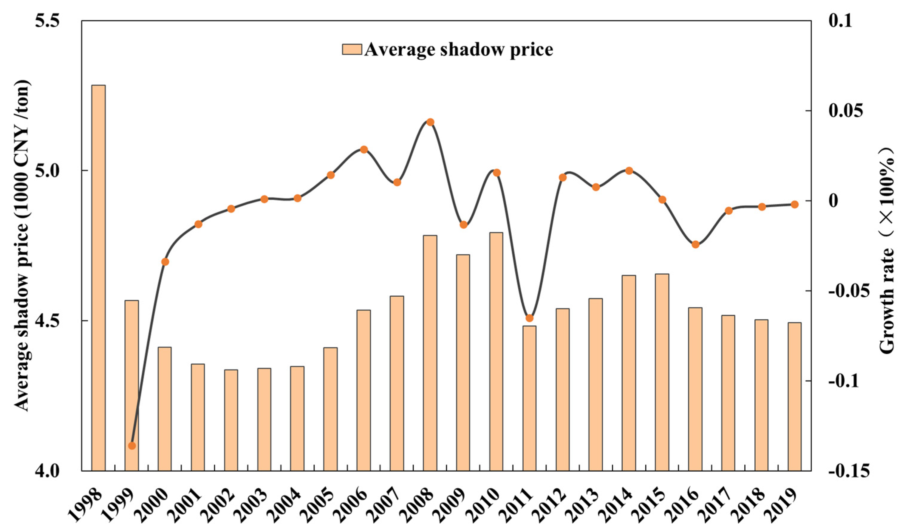
5.2. Shadow Price of Industrial CO₂

Figure 3 depicts the dynamic evolution process of the shadow price of industrial CO₂ from 1998 to 2019 (more details are shown in

Table A1. Shadow price of carbon dioxide in industrial sectors (CNY 1000/ton).

	1998	2001	2004	2007	2010	2013	2016	2019	Average MAC (CNY 1000/ton)	Average Carbon Intensity (CNY 10,000/ton)
ind01	12.966	7.706	7.791	8.551	8.339	8.157	6.724	5.220	7.935	1.881
ind02	3.951	3.570	3.587	3.580	3.720	3.591	3.747	3.721	3.672	1.628
ind03	3.666	3.642	3.661	3.684	3.662	3.616	3.625	3.544	3.640	1.190
ind04	3.843	3.744	3.696	3.719	3.688	3.638	3.607	3.551	3.678	0.452
ind05	4.004	3.789	3.733	3.719	3.723	3.669	3.678	3.569	3.726	1.532
ind06	4.417	4.131	4.073	4.169	4.336	4.013	4.154	3.662	4.113	0.414
ind07	4.094	3.894	3.943	4.010	4.140	4.160	4.193	4.069	4.056	0.647
ind08	4.085	3.910	3.833	3.845	3.921	3.964	3.984	3.797	3.909	0.687
ind09	3.514	3.490	3.441	3.426	3.408	3.365	3.417	3.427	3.431	0.119
ind10	17.984	8.649	9.366	11.866	11.538	6.345	5.776	5.055	9.030	0.442
ind11	4.892	5.027	5.949	7.606	8.073	7.658	7.078	5.262	6.505	0.185
ind12	4.148	4.171	4.631	5.229	5.378	5.447	5.179	4.636	4.881	0.129
ind13	3.871	3.747	3.840	4.008	4.099	3.951	3.950	3.731	3.897	0.486
ind14	3.686	3.649	3.768	3.945	4.030	4.013	4.035	4.024	3.890	0.150
ind15	4.284	4.034	3.988	4.009	4.043	3.927	3.874	3.880	3.992	1.229
ind16	3.938	3.771	3.793	3.833	3.883	3.872	3.891	3.847	3.842	0.186
ind17	3.866	3.854	4.025	4.170	4.221	4.610	4.641	4.286	4.200	0.294
ind18	3.597	3.391	3.209	3.077	2.965	2.900	3.161	3.252	3.173	1.449
ind19	6.755	5.190	4.592	4.369	4.423	3.880	3.982	3.617	4.519	1.468
ind20	3.999	4.067	3.979	4.022	4.115	4.129	4.207	4.106	4.064	0.293
ind21	3.708	3.650	3.578	3.557	3.570	3.570	3.536	3.599	3.592	0.452
ind22	3.914	3.795	3.787	3.851	3.892	3.725	3.744	3.706	3.800	0.335
ind23	4.161	4.026	4.215	4.580	4.955	4.536	4.547	4.482	4.433	0.137
ind24	15.874	6.925	6.449	6.351	6.556	5.722	5.948	5.041	6.733	10.366
ind25	5.263	4.492	3.818	3.317	3.247	3.368	3.593	3.303	3.741	8.938
ind26	4.041	3.933	3.668	3.438	3.471	3.319	3.353	3.417	3.572	0.828
ind27	4.725	4.293	4.368	4.753	5.151	4.935	4.928	5.174	4.748	0.287
ind28	7.075	5.249	5.153	5.747	6.457	5.495	5.437	5.283	5.627	0.357
ind29	5.496	4.551	4.557	4.673	4.932	4.772	4.777	4.747	4.760	0.261
ind30	5.986	4.904	4.507	4.630	4.885	4.954	5.109	5.261	4.993	0.144
ind31	4.903	4.411	4.691	5.423	6.628	6.164	6.243	5.997	5.557	0.081
ind32	3.996	3.775	3.881	5.336	8.692	11.054	10.997	17.036	7.932	0.035
ind33	3.877	3.750	3.822	3.929	4.022	3.899	3.892	3.832	3.879	0.077
ind34	4.311	4.268	3.795	3.275	3.127	3.028	3.281	3.322	3.527	26.711
ind35	3.609	3.587	3.571	3.556	3.532	3.529	3.526	3.578	3.555	1.434
ind36	3.748	3.752	3.754	3.721	3.745	3.704	3.724	3.763	3.737	0.164

). It is evident that the distribution of the shadow price of industrial CO₂ during the study period was mainly in the range of CNY 3~6 thousand/ton. The kernel density curve moves progressively to the right as time progresses. At the same time, the peak of the curve gradually decreases and the distribution of the shadow price becomes wider, indicating an expansion of the mean and variance of the shadow price distribution of CO₂ in the industrial sector.

As Figure 4 reveals, the average shadow price of industrial CO₂ in China showed a general downward trend between 1998 and 2019, falling from CNY 5285/ton to CNY 4494/ton—a decrease of 0.8%. Moreover, the mean shadow price of industrial CO₂ was CNY 4565/ton during the study period. This suggested that for the average Chinese industry, a reduction of 1 ton of CO₂ emissions would be accompanied by a reduction in gross industrial output of CNY 4565 at the current level of technology.

Specifically, during the study period, the shadow price of industrial CO₂ in China was broadly divided into three development stages: (1) The significantly declining stage (1998–2002): During this period, the shadow price of industrial CO₂ displayed a rapid downward trend, from CNY 5284.6/ton in 1998 to CNY 4336.0/ton in 2002, a cumulative decrease of 20.0%. As the government phased out and closed a total of over 100,000 small, technologically backward, energy-intensive and highly polluting companies in the mid-1990s, the survival of the fittest mechanism of market competition came into play and disorderly production was curbed. In 1997, the “Energy Conservation Law of the People’s Republic of China” was introduced. Since then, energy conservation and emission reduction have become a basic national policy, and carbon emission intensity has been effectively controlled and is now on a decreasing trend. (2) The slow growth stage (2002–2010): The shadow price of industrial CO₂ during this period rose from CNY 4340.5/ton in 2003 to CNY 4793.6/ton in 2010—an overall increase of only 10.4% and an average annual growth rate of 1.4%. In this period, China’s accession to the WTO and its export-oriented economic development mode gave rise to a large number of export-oriented light industries, such as textile industries, which led to cleaner production technology throughout the economy, causing a slight increase in the shadow price of CO₂. (3) The stage of a slow decline in fluctuation (2010–2019): During this period, the shadow price of industrial CO₂ decreased by CNY 299/ton, or 6.2%. In particular, it rose from CNY 4481.7/ton in 2011 to CNY 4655.0/ton in 2015 before slowly declining to CNY 4494.4/ton in 2019.

5.3. Shadow Price of CO₂ in Industrial Sectors

The above is a general overview of the shadow price of CO₂ in industrial sectors during 1998–2019. Further analysis of the shadow price of CO₂ and its trend over time for 36 industrial sectors is presented below, broken down by the industrial sector.

Figure 5 reveals that the shadow price of CO₂ varies considerably among the different industrial sectors during the study period. Of these 36 industrial industries, coal mining and dressing (ind01), the textile industry (ind10), garments and other fiber products (ind11), nonmetal mineral products (ind24) and electronic and telecommunications equipment (ind32) have a shadow price of CO₂ exceeding CNY 6000/ton. There are 12 industries with shadow prices of CO₂ between CNY 4000 and CNY 6000/ton, including the industries of leather, furs, down and related products (ind12); ordinary machinery (ind28); electric equipment and machinery (ind31), etc. Meanwhile, the shadow price of CO₂ is below CNY 4000/ton in 19 industries, such as petroleum processing and coking (ind18); smelting and pressing of ferrous metals (ind25); electric power, steam and hot water production and supply (ind34), etc.

Specifically, among the five industries with shadow prices of CO₂ exceeding CNY 6000/ton, the textile industry (ind10) records a significantly higher average shadow price of CO₂ than the other industries, with CNY 9030/ton. The coal mining and dressing (ind01) and electronic and telecommunications equipment (ind32) sectors are next to the textile sector at CNY 7935/ton and CNY 7932/ton, respectively. Evidently, industries with high shadow prices of CO₂ are mainly light industries and technology-intensive industries characterized by low carbon emissions, low pollution and high technology levels. Accordingly, these industries have little room for emission reduction and relatively greater difficulty in reducing emissions. The ordinary machinery sector (ind28) has the highest average shadow price of CO₂, amounting to CNY 5627/ton, while the food production sector (ind07) has the lowest at CNY 4056/ton. Of the 19 industries with a shadow price of CO₂ below CNY 4000/ton, the petroleum processing and coking industry (ind18) emerges at the bottom of the list at CNY 3173/ton. Furthermore, these 19 industries emit substantial amounts of carbon in the course of economic development, and the room for emission reduction is relatively large. Therefore, to achieve carbon emission reduction without affecting economic growth, we should focus on industries with low shadow prices of CO₂, and these 19 industries are good choices.

Figure 6 further depicts the tendency in the shadow price of CO₂ over time for different industrial sectors. As can be seen, the time-varying trends in the shadow price of CO₂ between 1998 and 2019 are clearly different for the different industrial sectors. Of the 36 industries, shadow prices trended upwards in 11 industries, downwards in 17 industries and remained unchanged in the other 8 industries.

Specifically, the shadow price of the electronic and telecommunications equipment sector (ind32) showed the most pronounced upward trend, with a cumulative increase of 326.3% and an annual growth rate of 3.3%, followed by the electric equipment and machinery (ind31), which saw its shadow price of CO₂ increase by 22.3%. However, there was a relatively moderate trend in the shadow price of CO₂ in sectors such as garments and other fiber products (ind11); leather, furs, down and related products (ind12); cultural, educational and sports articles (ind17); and metal products (ind27). In contrast, changes in the shadow price of CO₂ were more pronounced in industries such as textile (ind10), nonmetal mineral products (ind24), coal mining and dressing (ind01), and raw chemical materials and chemical products (ind19). In addition, the shadow price of CO₂ for gas production and supply (ind35) and tap water production and supply (ind36) remained essentially unchanged.

5.4. Influencing Factors of the Shadow Price

The above analysis reveals distinct differences between industries with regard to the shadow price of CO₂, namely, the marginal emission reduction cost. To account for this observation, it is necessary to further explore the potential factors affecting the marginal emission reduction cost of CO₂ from both theoretical and empirical studies. Existing studies [44] suggest that the shadow price of CO₂ has an “inverted U-shaped” relationship with the carbon emission intensity. This relationship can be used to estimate the marginal emission reduction cost, and thus, for policy simulation analysis. This paper takes into account the influence of the following factors on the marginal cost of CO₂ emission reductions:

(1)

Energy consumption structure (Ratio_coal). As an energy source with high carbon emission intensity, coal produces far more CO₂ than natural gas and oil. Therefore, this paper exposes the structure of energy consumption using the proportion of coal in total energy consumption with a view to measuring the impact of changes in the energy mix on reducing the marginal cost of CO₂.

(2)

Energy intensity (Inten_energy). Energy intensity is expressed as the proportion of energy consumption to total industrial output.

(3)

Carbon emission intensity (Inten_carbon). Generally, energy intensity and carbon emission intensity can be considered proxy variables for technological advances in energy use [45]. Therefore, carbon emission intensity is used to probe the relationship between different industries and the marginal reduction cost of CO₂ over time.

(4)

Industry type (Ratio_kl). In this paper, the ratio of capital input to labor input is used to determine the industry type. A lower ratio of capital to labor indicates a more labor-intensive industry, while a higher ratio means that the industry is more capital-intensive. Typically, higher capital–labor ratios imply superior production technology, which will further affect the marginal cost of CO₂ reduction.

According to the preceding analysis, this assay takes the marginal reduction cost of CO₂ as the explained variable, represented by $y_{i,t}$, and the above four potential influencing factors as explanatory variables, represented by $Z_{i,t}$, and constructs the panel regression model as follows:

$$y_{i,t}=\alpha +\beta x^2{}_{i,t}+\gamma x_{i,t}+\eta Z_{i,t}+{\lambda }_t+{\mu }_i+{\epsilon }_{i,t}$$

(20)

where $\alpha ,\beta ,\gamma ,\eta$ are regression coefficients, ${\lambda }_t$ is the time effect, ${\mu }_i$ is the individual effect, and ${\epsilon }_{i,t}$ is the error term. Descriptive statistics of the above variables are shown in

Table 4. Descriptive statistics of variables.

Variable.	Samples	Mean	Std.	Min.	Max.
Mac	792	4.565	1.722	2.859	17.984
Inten_carbon	792	0.018	0.049	0	0.429
Inten_carbon2	792	0.003	0.014	0	0.184
Inten_energy	792	2.957	5.675	0.042	34.407
Ratio coal	792	0.693	1.094	0.005	7.599
Ratio kl	792	28.027	38.472	2.185	325.6

.

To avoid multicollinearity among influencing factors, different covariates were gradually added to the regression model for comparison, and the optimal regression model was selected by in-sample fitting criteria and out-of-sample prediction criteria. Considering the large inter-industry variation and the possible serial correlation of marginal CO₂ emission reduction costs, this paper adopts the feasible generalized least square (FGLS) method for estimation, and the detailed regression outcomes are exhibited in

Table 5. The regression results of MACC.

	(1)	(2)	(3)	(4)
Inten_carbon	17.157 **	24.332 ***	24.127 ***	24.927 ***
	(7.573)	(7.432)	(7.425)	(7.400)
Inten_carbon2	−27.221 *	−34.837 **	−35.868 **	−30.109 **
	(14.387)	(14.023)	(14.029)	(14.145)
Inten_energy		−0.112 ***	−0.108 ***	−0.100 ***
		(0.016)	(0.017)	(0.017)
Ratio_coal			−0.239	−0.086
			(0.179)	(0.188)
Ratio_kl				−0.006 ***
				(0.002)
Constant	5.402 ***	5.271 ***	5.366 ***	5.278 ***
	(0.268)	(0.262)	(0.271)	(0.272)
Observations	792	792	792	792
Number of id	36	36	36	36
Wald	1590	1732	1737	1759
AIC	2353.268	2309.636	2309.867	2305.177
BIC	2629.067	2590.11	2595.015	2590
RAE	0.436	0.423	0.421	0.417
RMSFE	0.992	0.964	0.963	0.959

Standard errors in parentheses. *** p < 0.01, ** p < 0.05, * p < 0.1.

. It is evident that the non-linear relationship between marginal CO₂ emission reduction cost and carbon emission intensity is robust. At the significance level of 1%, the coefficients for carbon emission intensity are all positive and those for the secondary terms are all negative. The significance level increases from 10% to 5% with the gradual addition of control variables.

Specifically, model (1) only includes carbon emission intensity and its secondary term as explanatory variables, providing a simple exploration of the association between marginal CO₂ emission reduction costs and carbon emission intensity. The outcomes uncover that the coefficient of carbon emission intensity is positive at the significance level of 5%, and the coefficient of the secondary term is negative at the significance level of 10%. Furthermore, marginal CO₂ emission reduction costs have a distinct inverted U-shaped relationship with carbon emission intensity. In parallel, control variables were gradually added to exclude the impacts of other missing variables. Based on model (1), the energy intensity variable is included in the regression analysis in model (2). Regression results point to a significant negative effect of energy intensity on CO₂ emission reduction costs, which is in line with expectations. The quadratic coefficient of carbon emission intensity remains negative, with a sharp increase in significance from 10% to 5%, which further verifies the inverted U-shaped relationship between the CO₂ emission reduction costs and carbon emission intensity. In model (3), energy structure variables are further incorporated into the regression analysis on the basis of model (2). The estimated results show that the share of coal in energy consumption negatively affects CO₂ emission reduction costs. That is, an expansion in the ratio of coal to energy consumption will lead to a decrease in the CO₂ emission reduction costs, but the coefficient of this variable is not significant. In model (4), the industry-type variable was further added to clarify the impact of industry type on CO₂ emission reduction costs. As Table 5 depicts, the regression coefficient of the industry-type variable is significantly negative at the 1% level. Additionally, a time dummy variable is added to model (4) to eliminate the impact of technological progress on CO₂ reduction costs. The results demonstrated that there remains a remarkable inverted U-shaped association between CO₂ emission reduction costs and carbon emission intensity despite controlling for time trends.

The last four rows in Table 5 report the results of the regression in-sample fitting criteria and out-of-sample prediction criteria. AIC and BIC are usually used to compare the goodness of fit in a sample. The smaller the AIC and BIC values are, the better the model fit. For out-of-sample predictions, smaller MAE and RMSFE values yield smaller prediction errors and more accurate results. It is clear from the table that model (4) is the best-fitting model, both in terms of in-sample fit criteria and out-of-sample prediction criteria. Therefore, model (4) can be used to estimate the marginal cost curve of CO₂ emission reduction. The inflection point of the marginal cost curve of CO₂ emission reduction, namely, the critical value, can be calculated as 0.41 tons/CNY 10,000.

Figure 7 simulates the marginal CO₂ emission reduction cost curve of the industrial sector. As can be seen, marginal CO₂ emission reduction costs will rise with the increase of carbon emission intensity provided that the industrial carbon emission intensity is less than the threshold value of 0.41 tons/CNY 10,000, which means a cleaner production technology. In contrast, when the industrial carbon emission intensity is greater than 0.41 tons/CNY 10,000, the marginal CO₂ emission reduction cost will decrease with the elevation of carbon emission intensity, and the production technology will become less clean.

Compared with the average carbon emission intensity of industrial sectors (see Table A1), a total of 17 industries have a carbon emission intensity of less than 0.41 tons/CNY 10,000, including the tobacco processing sector (ind09); the furniture manufacturing sector (ind14); the culture, educational, and sports articles (ind17); and the electronic and telecommunications equipment (ind32). This implies that the production technology will become cleaner even if the carbon emission intensity of these industries increases in the short term as long as the threshold is not exceeded. The remaining 19 industries, especially high-emitting sectors such as smelting and pressing of ferrous metals (ind25) and electric power, steam and hot water production and supply (ind34), have carbon emission intensifies much higher than 0.41 tons/CNY 10,000, implying that production technologies will become dirtier as carbon emission intensifies increase further. The research results show that industries with high marginal emission reduction costs have low carbon emission intensity and vice versa [46], which confirms the findings of this paper.

6. Conclusions

Based on the directional distance function, this paper adopts parametric linear programming and the Bayes bootstrap estimation method to more scientifically and accurately measure the marginal CO₂ emission reduction cost of 36 industrial sectors in China from 1998 to 2019 and provides a detailed analysis from the perspective of time trend and industry differences. The marginal reduction cost curve for the industry is further fitted by constructing a panel regression model. The findings of this article are listed as follows:

(1)

The parameter estimates modified by the Bayes bootstrap estimation method are significantly higher than the original parameter estimates solved by the linear programming method, indicating that ignoring the influence of random disturbances on the production frontier leads to biased model parameters and does accurately predict the shadow price of CO₂.

(2)

The average deviation-corrected shadow price of CO₂ is CNY 4565/ton, which has roughly evolved three stages in terms of time trends: the significantly declining stage (1998~2002), the slow growth stage (2002~2010) and the stage of a slow decline in fluctuation (2010~2019). The shadow price of CO₂ varied greatly by industry, with the textile industry having the highest average shadow price of CO₂ at CNY 9030/ton, as opposed to the lowest in the petroleum processing and coking industry at CNY 3173/ton. Moreover, the trend in the shadow price of CO₂ over time in different industries reveals that more industries are becoming cleaner.

(3)

The fitting results of the CO₂ marginal emission reduction cost curve show that the shadow price of CO₂ has an “inverted U-shaped” relationship with the carbon emission intensity. The marginal CO₂ emission reduction cost will rise with the increase in carbon emission intensity, provided that the industrial carbon emission intensity is less than the threshold value of 0.41 tons/CNY 10,000, which means a cleaner production technology. In contrast, when the industrial carbon emission intensity is greater than 0.41 tons/CNY 10,000, the marginal CO₂ emission reduction cost will decrease with the enhancement in carbon emission intensity, and the production technology will become less clean.

According to the above conclusions, some important policy implications are drawn. First, the shadow price of carbon dioxide varies considerably between sectors, which means that it is more efficient to reduce emissions through market mechanisms. Therefore, within the constraint of the 2030 carbon intensity target, the government can allocate carbon emission permits to various industries following the principles of equity and efficiency. In addition, when setting emission reduction targets for different industrial sectors, the government can allocate more emission reduction tasks to high-emission industries with lower shadow prices on the right side of the critical value, or set its emission reduction targets with a critical value as the benchmark.

The limitation of this paper is that only four potential variables, namely, energy consumption structure, energy intensity, carbon emission intensity and industry type, were considered when studying the influencing factors of marginal emission reduction costs. Therefore, further research should include more variables such as per capita industrial output, industrial structure, and the number of private cars in order to more accurately determine the impact of economic development on marginal emission reduction costs.

References

1. Xu, H.; Pan, X.; Li, J.; Feng, S.; Guo, S. Comparing the impacts of carbon tax and carbon emission trading, which regulation is more effective? J. Environ. Manag. 2023, 330, 117156. [Google Scholar] [CrossRef] [PubMed]
2. Peng, J.; Yu, B.-Y.; Liao, H.; Wei, Y.-M. Marginal abatement costs of CO2 emissions in the thermal power sector: A regional empirical analysis from China. J. Clean. Prod. 2018, 171, 163–174. [Google Scholar] [CrossRef]
3. Huang, G.; Ouyang, X.; Yao, X. Dynamics of China’s regional carbon emissions under gradient economic development mode. Ecol. Indic. 2015, 51, 197–204. [Google Scholar] [CrossRef]
4. Wang, K.; Wei, Y.M. China’s regional industrial energy efficiency and carbon emissions abatement costs. Appl. Energy 2014, 130, 617–631. [Google Scholar] [CrossRef]
5. Wei, C.; Löschel, A.; Liu, B. An empirical analysis of the CO2 shadow price in Chinese thermal power enterprises. Energy Econ. 2013, 40, 22–31. [Google Scholar] [CrossRef]
6. Shen, Z.; Li, R.; Baležentis, T. The patterns and determinants of the carbon shadow price in China’s industrial sector: A by-production framework with directional distance function. J. Clean. Prod. 2021, 323, 129175. [Google Scholar] [CrossRef]
7. Jin, Y.; Chen, B. Comparison of potential CO2 reduction and marginal abatement costs across in the China and Korea manufacturing industries. J. Innov. Knowl. 2022, 7, 100172. [Google Scholar] [CrossRef]
8. Zhou, X.; Fan, L.W.; Zhou, P. Marginal CO2 abatement costs: Findings from alternative shadow price estimates for Shanghai industrial sectors. Energy Policy 2015, 77, 109–117. [Google Scholar] [CrossRef]
9. Wang, Y.; Geng, S.; Zhao, P.; Du, H.; He, Y.; Crittenden, J. Cost–benefit analysis of GHG emission reduction in waste to energy projects of China under clean development mechanism. Resour. Conserv. Recycl. 2016, 109, 90–95. [Google Scholar] [CrossRef]
10. Zhang, Z.X.; Folmer, H. Economic modelling approaches to cost estimates for the control of carbon dioxide emissions. Energy Econ. 1998, 20, 101–120. [Google Scholar] [CrossRef]
11. Yu, S.; Zhang, J.; Cheng, J. Carbon reduction cost estimating of Chinese coal-fired power generation units: A perspective from national energy consumption standard. J. Clean. Prod. 2016, 139, 612–621. [Google Scholar] [CrossRef]
12. Morris, J.; Paltsev, S.; Reilly, J. Marginal abatement costs and marginal welfare costs for greenhouse gas emissions reductions: Results from the EPPA model. Environ. Model. Assess. 2012, 17, 325–336. [Google Scholar] [CrossRef]
13. Pereira, A.M.; Pereira, R.M.M. Is fuel-switching a no-regrets environmental policy? VAR evidence on carbon dioxide emissions, energy consumption and economic performance in Portugal. Energy Econ. 2010, 32, 227–242. [Google Scholar] [CrossRef]
14. Wang, G.Y.; Li, Y.P.; Liu, J.; Huang, G.H.; Chen, L.R.; Yang, Y.J.; Gao, P.P. A two-phase factorial input-output model for analyzing CO2-emission reduction pathway and strategy from multiple perspectives–A case study of Fujian province. Energy 2022, 248, 123615. [Google Scholar] [CrossRef]
15. Hannum, C.; Cutler, H.; Iverson, T.; Keyser, D. Estimating the implied cost of carbon in future scenarios using a CGE model: The Case of Colorado. Energy Policy 2017, 102, 500–511. [Google Scholar] [CrossRef]
16. Tanatvanit, S.; Limmeechokchai, B.; Shrestha, R.M. CO2 mitigation and power generation implications of clean supply-side and demand-side technologies in Thailand. Energy Policy 2004, 32, 83–90. [Google Scholar] [CrossRef]
17. Choi, Y.; Zhang, N.; Zhou, P. Efficiency and abatement costs of energy-related CO2 emissions in China: A slacks-based efficiency measure. Appl. Energy 2012, 98, 198–208. [Google Scholar] [CrossRef]
18. Färe, R.; Grosskopf, S.; Weber, W.L. Shadow prices and pollution costs in US agriculture. Ecol. Econ. 2006, 56, 89–103. [Google Scholar] [CrossRef]
19. Xie, B.C.; Duan, N.; Wang, Y.S. Environmental efficiency and abatement cost of China’s industrial sectors based on a three-stage data envelopment analysis. J. Clean. Prod. 2017, 153, 626–636. [Google Scholar] [CrossRef]
20. Sun, Z.; Luo, R.; Zhou, D. Optimal path for controlling sectoral CO2 emissions among China’s regions: A centralized DEA approach. Sustainability 2015, 8, 28. [Google Scholar] [CrossRef]
21. Wu, J.; Yin, P.; Sun, J.; Chu, J.; Liang, L. Evaluating the environmental efficiency of a two-stage system with undesired outputs by a DEA approach: An interest preference perspective. Eur. J. Oper. Res. 2016, 254, 1047–1062. [Google Scholar] [CrossRef]
22. Cecchini, L.; Venanzi, S.; Pierri, A.; Chiorri, M. Environmental efficiency analysis and estimation of CO2 abatement costs in dairy cattle farms in Umbria (Italy): A SBM-DEA model with undesirable output. J. Clean. Prod. 2018, 197, 895–907. [Google Scholar] [CrossRef]
23. Baležentis, T.; Dabkienė, V.; Štreimikienė, D. Eco-efficiency and shadow price of greenhouse gas emissions in Lithuanian dairy farms: An application of the slacks-based measure. J. Clean. Prod. 2022, 356, 131857. [Google Scholar] [CrossRef]
24. Lee, J.D.; Park, J.B.; Kim, T.Y. Estimation of the shadow prices of pollutants with production/environment inefficiency taken into account: A nonparametric directional distance function approach. J. Environ. Manag. 2002, 64, 365–375. [Google Scholar] [CrossRef] [PubMed]
25. Färe, R.; Grosskopf, S.; Noh, D.-W.; Weber, W. Characteristics of a polluting technology: Theory and practice. J. Econom. 2005, 126, 469–492. [Google Scholar] [CrossRef]
26. Marklund, P.O.; Samakovlis, E. What is driving the EU burden-sharing agreement: Efficiency or equity? J. Environ. Manag. 2007, 85, 317–329. [Google Scholar] [CrossRef]
27. Liu, J.Y.; Feng, C. Marginal abatement costs of carbon dioxide emissions and Its influencing factors: A global perspective. J. Clean. Prod. 2018, 170, 1433–1450. [Google Scholar] [CrossRef]
28. Xue, Z.; Mu, H.; Li, N.; Zhang, M. Analysis on shadow price and abatement potential of carbon dioxide in China’s provincial industrial sectors. Environ. Sci. Pollut. Res. 2022, 29, 14604–14623. [Google Scholar] [CrossRef]
29. Wang, F.; Wang, R.; Nan, X. Marginal abatement costs of industrial CO2 emissions and their influence factors in China. Sustain. Prod. Consum. 2022, 30, 930–945. [Google Scholar] [CrossRef]
30. Yang, K.; Lei, Y. The carbon dioxide marginal abatement cost calculation of Chinese provinces based on stochastic frontier analysis. Nat. Hazards 2017, 85, 505–521. [Google Scholar] [CrossRef]
31. Zhang, N.; Huang, X.; Liu, Y. The cost of low-carbon transition for China’s coal-fired power plants: A quantile frontier approach. Technol. Forecast. Soc. Chang. 2021, 169, 120809. [Google Scholar] [CrossRef]
32. Liu, Q.; Qi, R.; Zhao, Y.; Zhou, T. Comparative analysis of the marginal abatement cost modeling for coal-fired power plants in China. J. Clean. Prod. 2022, 356, 131883. [Google Scholar] [CrossRef]
33. Zhang, N.; Huang, X.; Qi, C. The effect of environmental regulation on the marginal abatement cost of industrial firms: Evidence from the 11th Five-Year Plan in China. Energy Econ. 2022, 112, 106147. [Google Scholar] [CrossRef]
34. Qi, C.; Choi, Y. A study of the feasibility of international ETS cooperation between Shanghai and Korea from environmental efficiency and CO2 marginal abatement cost perspectives. Sustainability 2019, 11, 4468. [Google Scholar] [CrossRef]
35. Ackerberg, D.A.; Caves, K.; Frazer, G. Identification properties of recent production function estimators. Econometrica 2015, 83, 2411–2451. [Google Scholar] [CrossRef]
36. Yang, M.; Xu, J.; Li, M.; Duan, H. A bootstrap assessment of the shadow prices of CO2 for the industrial sector in China’s key cities. Clim. Change Econ. 2021, 12, 2150015. [Google Scholar] [CrossRef]
37. Färe, R.; Lundberg, A. Parameterizing the Shortage Function; Mimeo, Department of Economics, Oregon State University: Corvallis, OR, USA, 2006. [Google Scholar]
38. Färe, R.; Grosskopf, S.; Hayes, K.J.; Margaritis, D. Estimating demand with distance functions: Parameterization in the primal and dual. J. Econom. 2008, 147, 266–274. [Google Scholar] [CrossRef]
39. Färe, R.; Martins-Filho, C.; Vardanyan, M. On functional form representation of multi-output production technologies. J. Product. Anal. 2010, 33, 81–96. [Google Scholar] [CrossRef]
40. Aigner, D.J.; Chu, S. On estimating the industry production function. Am. Econ. Rev. 1968, 58, 826–839. [Google Scholar]
41. Li, K.; Lin, B. Metafroniter energy efficiency with CO2 emissions and its convergence analysis for China. Energy Econ. 2015, 48, 230–241. [Google Scholar] [CrossRef]
42. Zhang, J. Estimation of China’s provincial capital stock (1952–2004) with applications. J. Chin. Econ. Bus. Stud. 2008, 6, 177–196. [Google Scholar] [CrossRef]
43. Eggleston, S.; Buendia, L.; Miwa, K. 2006 IPCC Guidelines for National Greenhouse Gas Inventories; Institute for Global Environmental Strategies: Hayama, Japan, 2006. [Google Scholar]
44. Du, L.; Hanley, A.; Wei, C. Marginal abatement costs of carbon dioxide emissions in China: A parametric analysis. Environ. Resour. Econ. 2015, 61, 191–216. [Google Scholar] [CrossRef]
45. Fan, Y.; Liu, L.-C.; Wu, G.; Wei, Y.-M. Analyzing impact factors of CO2 emissions using the STIRPAT model. Environ. Impact Assess. Rev. 2006, 26, 377–395. [Google Scholar] [CrossRef]
46. Xiao, B.; Niu, D.; Wu, H.; Wang, H. Marginal abatement cost of CO2 in China based on directional distance function: An industry perspective. Sustainability 2017, 9, 138. [Google Scholar] [CrossRef]
Figure 1. Research framework of this paper.
Sustainability 15 08662 g001
Figure 2. Directional distance function.
Sustainability 15 08662 g002
Figure 3. The kernel density curve of the shadow price of industrial CO2.
Sustainability 15 08662 g003
Figure 4. The mean shadow price of industrial CO2 (CNY 1000/ton).
Sustainability 15 08662 g004
Figure 5. The average shadow price of CO2 in industrial sectors (CNY 1000/ton).
Sustainability 15 08662 g005
Figure 6. The shadow price of CO2 in different industrial sectors (CNY 1000/ton).
Sustainability 15 08662 g006
Figure 7. MACC of the industrial sector.
Sustainability 15 08662 g007