
Seascape Visual Characterization: Combining Viewing Geometry and Physical Features to Quantify the Perception of Seascape

Abstract
:1. Introduction
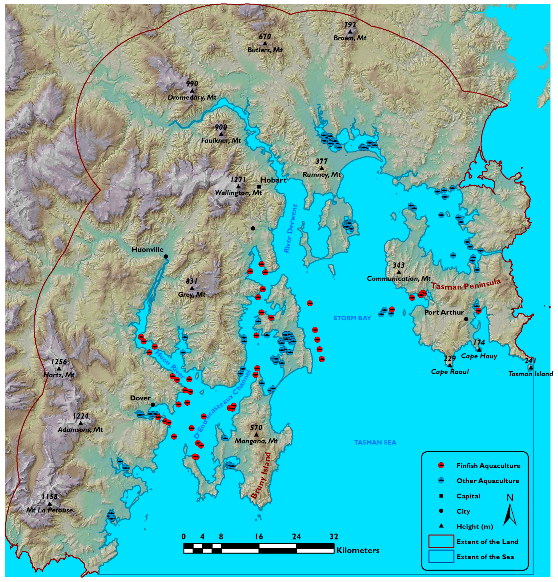
2. Study Region
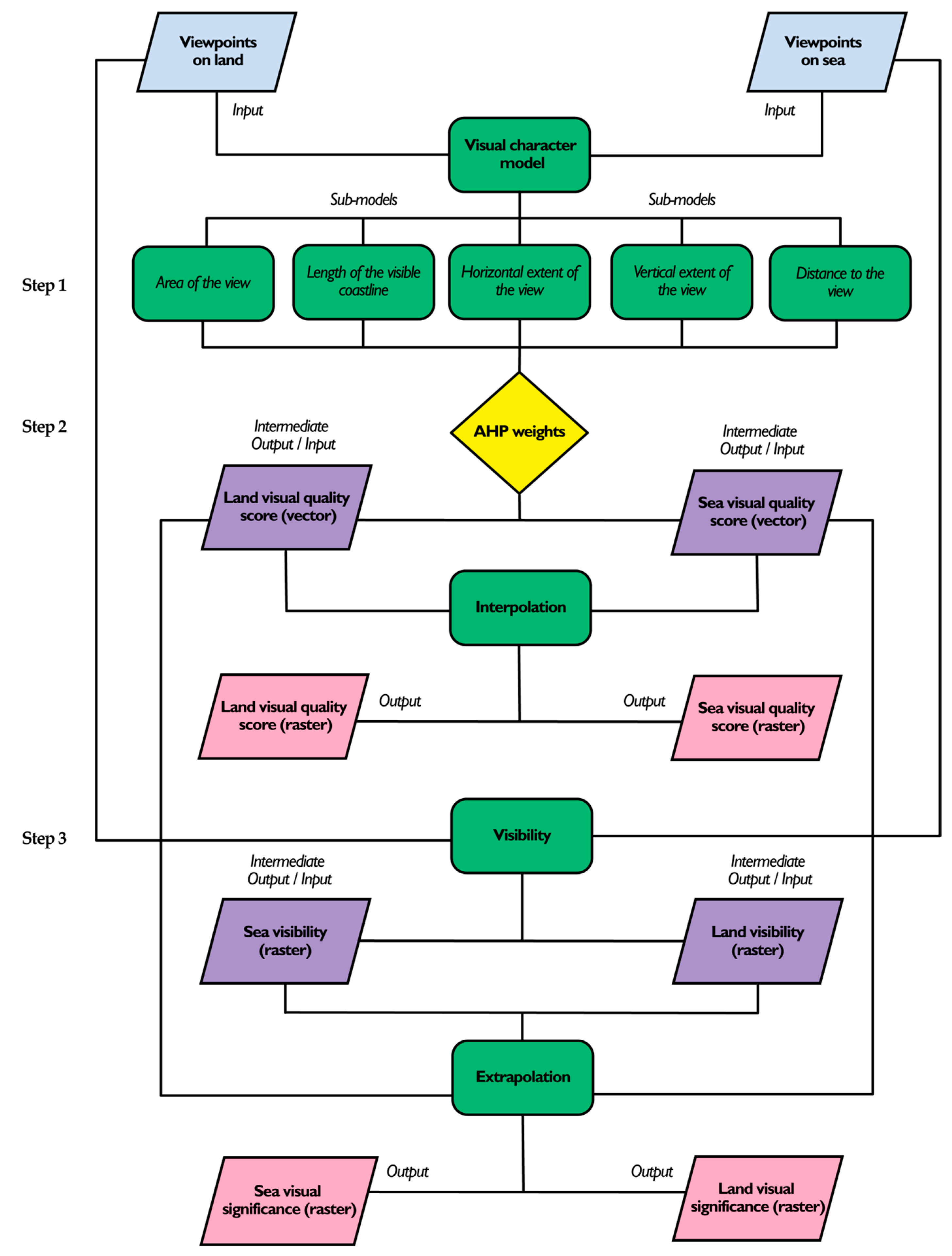
3. Model Components and Development
3.1. Establishing the Visual Character Model Environment
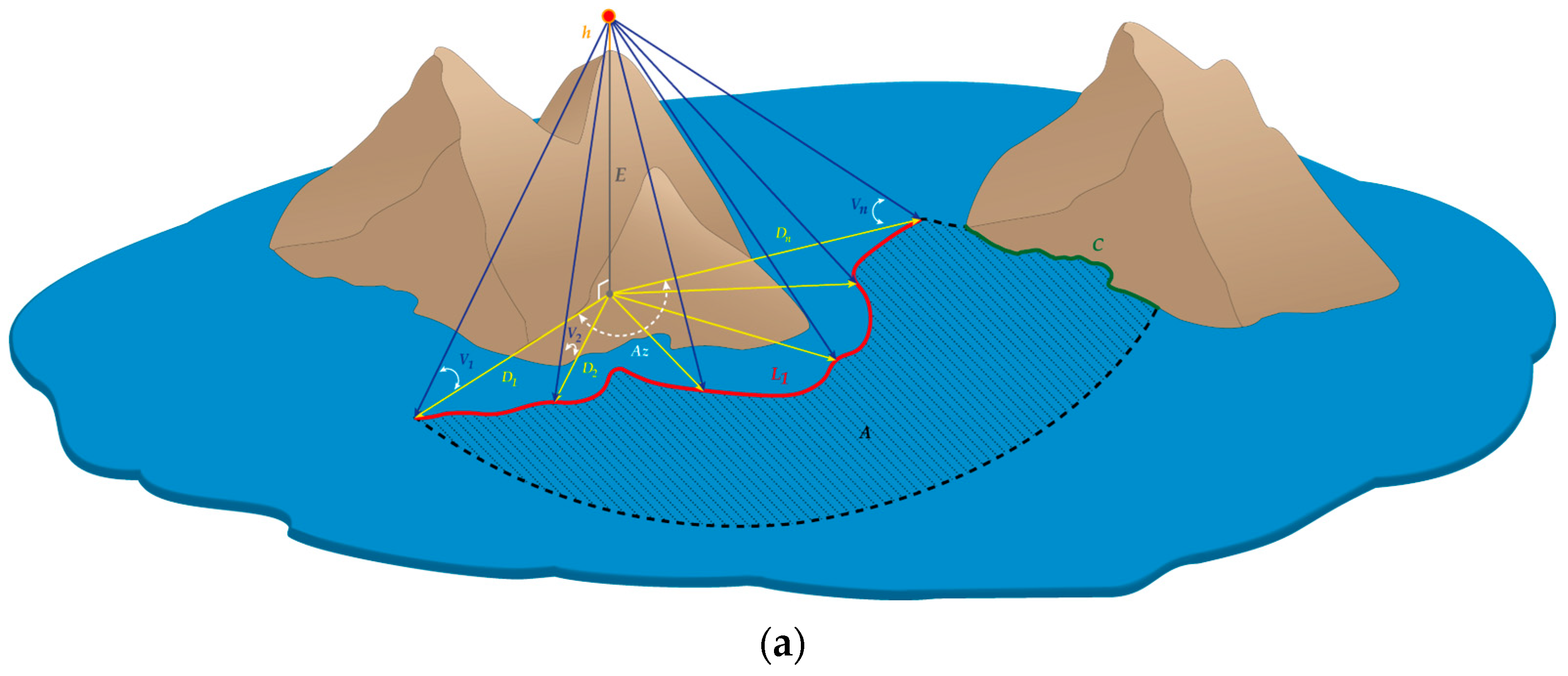
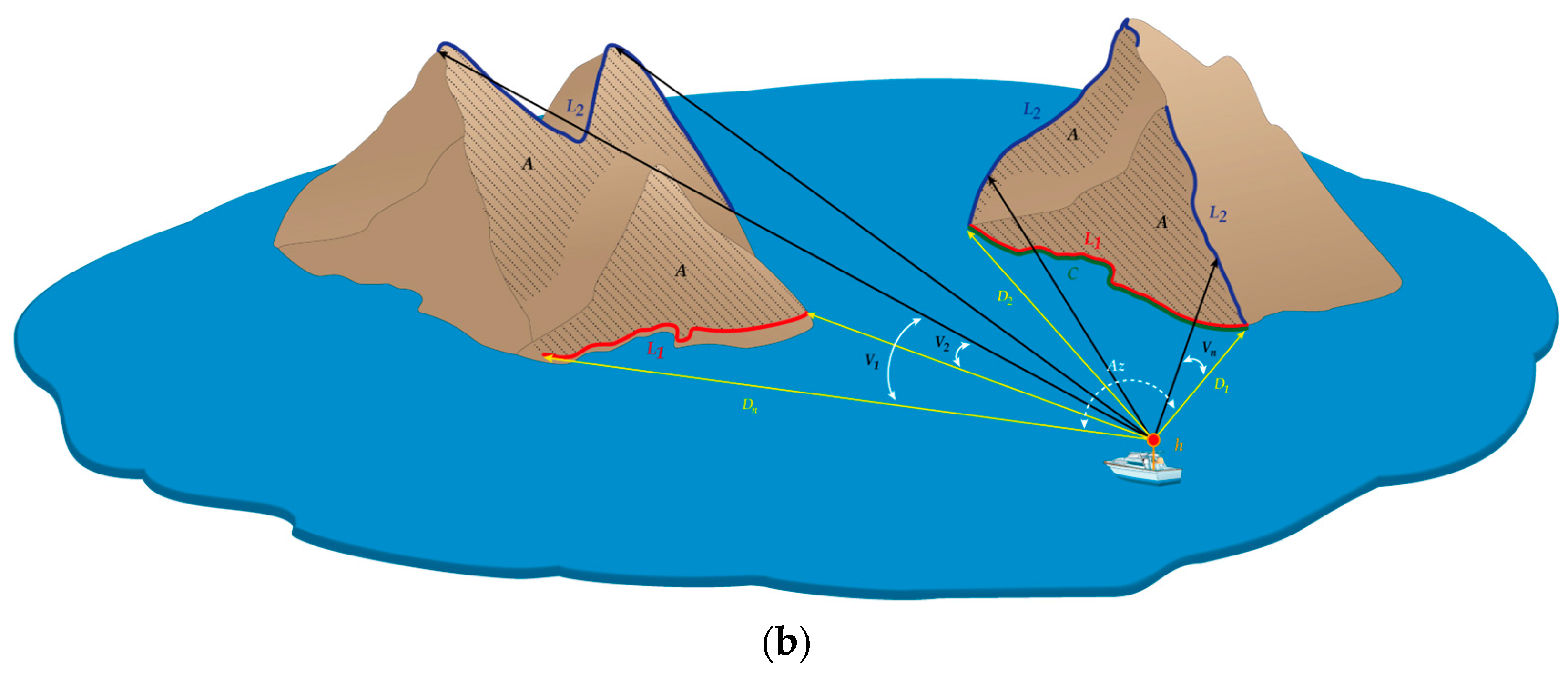
3.2. Stage One: Seascape Visual Character Model
3.2.1. Area of Visibility
3.2.2. Length of the Visible Coastline
3.2.3. Horizontal Extent of the View
3.2.4. Vertical Extent of the View
3.2.5. Distance to the View
3.3. Second Stage: Seascape Visual Perceptual Quality Score
3.4. Stage Three: Synthesis
4. Results
5. Discussion
6. Conclusions
Author Contributions
Funding
Institutional Review Board Statement
Informed Consent Statement
Data Availability Statement
Acknowledgments
Conflicts of Interest
References
- Hill, M.; Briggs, J.; Minto, P.; Bagnall, D.; Foley, K.; Williams, A. Guide to Best Practice in Seascape Assessment; Marine Institute: Rinville, Ireland, 2001. [Google Scholar]
- Eikeset, A.M.; Mazzarella, A.B.; Davíðsdóttir, B.; Klinger, D.H.; Levin, S.A.; Rovenskaya, E.; Stenseth, N.C. What is blue growth? The semantics of “Sustainable Development” of marine environments. Mar. Policy 2018, 87, 177–179. [Google Scholar] [CrossRef]
- Hoerterer, C.; Schupp, M.F.; Benkens, A.; Nickiewicz, D.; Krause, G.; Buck, B.H. Stakeholder Perspectives on Opportunities and Challenges in Achieving Sustainable Growth of the Blue Economy in a Changing Climate. Front. Mar. Sci. 2020, 6, 795. [Google Scholar] [CrossRef]
- Maslov, N.; Claramunt, C.; Wang, T.; Tang, T. Evaluating the Visual Impact of an Offshore Wind Farm. Energy Procedia 2017, 105, 3095–3100. [Google Scholar] [CrossRef]
- Falconer, L.; Hunter, D.-C.; Telfer, T.C.; Ross, L.G. Visual, seascape and landscape analysis to support coastal aquaculture site selection. Land Use Policy 2013, 34, 1–10. [Google Scholar] [CrossRef]
- Devine-Wright, P.; Howes, Y. Disruption to place attachment and the protection of restorative environments: A wind energy case study. J. Environ. Psychol. 2010, 30, 271–280. [Google Scholar] [CrossRef]
- Depellegrin, D.; Blazauskas, N.; Egarter-Vigl, L. An integrated visual impact assessment model for offshore windfarm development. Ocean Coast Manag. 2014, 98, 95–110. [Google Scholar] [CrossRef]
- Morris, P.; Therivel, R. Methods of Environmental Impact Assessment, 3rd ed.; Routledge: London, UK, 2009. [Google Scholar] [CrossRef]
- Natural England. An Approach to Seascape Character Assessment; NECR105; Bristol, UK, 2012. Available online: https://assets.publishing.service.gov.uk/government/uploads/system/uploads/attachment_data/file/396177/seascape-character-assessment.pdf (accessed on 13 March 2023).
- Briggs, J.; White, S. Welsh Seascapes and Their Sensitivity to Offshore Developments: Method Report; Countryside Council for Wales (CCW): Bangor, UK, 2009.
- Parker, S.K.A.; Grant, A.; Ahern, K. National Seascape Assessment for Wales; NRW Evidence Report 80; Wales, UK, 2015. Available online: https://naturalresources.wales/media/682028/mca-00-technical-report-summary-method-appendix.pdf (accessed on 13 March 2023).
- MMO. Seascape Assessment for the South Marine Plan Areas: Technical Report; MMO 1037; Marine Management Organisation: Newcastle, UK, 2014; p. 88.
- DTI. Guidance on the Assessment of the Impact of Offshore Wind Farms: Seascape and Visual Impact Report; 806666; UK, 2005. Available online: http://www.dti.gov.uk/renewables/pdfs/seascape_rep.pdf (accessed on 13 March 2023).
- Miller, D.R.; Morrice, J.G. A Geographical Analysis of the Intervisibility of the Coastal Areas of Wales for Characterizing Seascapes; INTERREG 1994–1999; UK, 2001. Available online: https://www.hutton.ac.uk/sites/default/files/files/Geographic%20Analysis%20of%20Seascapes%20of%20Wales%20Miller%20and%20Morrice%20April%202002.pdf (accessed on 13 March 2023).
- Fry, G.; Tveit, M.S.; Ode, A.; Velarde, M.D. The ecology of visual landscapes: Exploring the conceptual common ground of visual and ecological landscape indicators. Ecol. Indic. 2009, 9, 933–947. [Google Scholar] [CrossRef]
- Tveit, M.; Ode, A.; Fry, G. Key concepts in a framework for analysing visual landscape character. Landsc. Res. 2006, 31, 229–255. [Google Scholar] [CrossRef]
- Gkoltsiou, A.; Mougiakou, E. The use of Islandscape character assessment and participatory spatial SWOT analysis to the strategic planning and sustainable development of small islands. The case of Gavdos. Land Use Policy 2021, 103, 105277. [Google Scholar] [CrossRef]
- Tsilimigkas, G.; Rempis, N.; Derdemezi, E.T. Marine Zoning and Landscape Management on Crete Island, Greece. J. Coast. Conserv. 2020, 24, 43. [Google Scholar] [CrossRef]
- López-Sánchez, N.; Niveau-de-Villedary y Mariñas, A.M.; Gómez-González, J.I. The Shrines of Gadir (Cadiz, Spain) as References for Navigation. GIS Visibility Anal. 2019, 5, 284–308. [Google Scholar] [CrossRef]
- Taofiqurohman, A.; Radjawane, I.M.; Dhahiyat, Y. Aesthetic quality assessment in Santolo Beach, West Java Province, Indonesia. IOP Conf. Ser. Earth Environ. Sci. 2018, 162, 012029. [Google Scholar] [CrossRef]
- Depellegrin, D. Assessing cumulative visual impacts in coastal areas of the Baltic Sea. Ocean. Coast Manag. 2016, 119, 184–198. [Google Scholar] [CrossRef]
- Kaplan, S. An informal model for the prediction of preference. In Landscape Asessment: Values, Perception and Resources; Zube, E.H., Brush, R.O., Fabos, J.G., Eds.; Dowden, Hutchinson and Ross: Stroudsburg, PA, USA, 1975; pp. 92–101. [Google Scholar]
- Martin, B.; Ortega, E.; Otero, I.; Arce, R.M. Landscape character assessment with GIS using map-based indicators and photographs in the relationship between landscape and roads. J. Env. Manag. 2016, 180, 324–334. [Google Scholar] [CrossRef]
- Sullivan, R.; Kirchler, L.; Lahti, T.; Roché, S.; Beckman, K.; Cantwell, B.; Richmond, P. Wind Turbine Visibility and Visual Impact Threshold Distances in Western Landscapes. In Proceedings of the National Association of Environmental Professionals 37th Annual Conference, Portland, OR, USA, 21–24 May 2012. [Google Scholar]
- Mouflis, G.D.; Gitas, I.Z.; Iliadou, S.; Mitri, G.H. Assessment of the visual impact of marble quarry expansion (1984–2000) on the landscape of Thasos island, NE Greece. Landsc. Urban Plan. 2008, 86, 92–102. [Google Scholar] [CrossRef]
- Kaplan, S. Perception and landscape: Conceptions and misconceptions. In Environmental Aesthetics: Theory, Research, and Application; Nasar, J.L., Ed.; Cambridge University Press: Cambridge, UK, 1988; pp. 45–55. [Google Scholar] [CrossRef]
- Cakci, I. Landscape Perception. Landsc. Plan. 2012, 251–276. [Google Scholar] [CrossRef]
- Sevenant, M.; Antrop, M. Landscape Representation Validity: A Comparison between On-site Observations and Photographs with Different Angles of View. Landsc. Res. 2011, 36, 363–385. [Google Scholar] [CrossRef]
- ASH design + assessment. Landscape/Seascape Capacity for Aquaculture: Outer Hebrides Pilot Study; No. 460; Scottish Natural Heritage Commissioned: Inverness, UK, 2011. [Google Scholar]
- Pinkau, A.; Schiele, K.S. Strategic Environmental Assessment in marine spatial planning of the North Sea and the Baltic Sea–An implementation tool for an ecosystem-based approach? Mar. Policy 2021, 130, 104547. [Google Scholar] [CrossRef]
- ESRI. Viewshed (Spatial Analyst). Available online: https://pro.arcgis.com/en/pro-app/latest/tool-reference/spatial-analyst/viewshed.htm (accessed on 10 April 2023).
- ESRI. Line Of Sight (3D Analyst). Available online: https://pro.arcgis.com/en/pro-app/latest/tool-reference/3d-analyst/line-of-sight.htm (accessed on 10 April 2023).
- ESRI. Skyline (3D Analyst). Available online: https://pro.arcgis.com/en/pro-app/latest/tool-reference/3d-analyst/skyline.htm (accessed on 10 April 2023).
- Tasmanian Government. The Perfect Environment for an Innovative and Successful Aquaculture Industry. Available online: www.cg.tas.gov.au (accessed on 1 October 2022).
- Land Information System Tasmania. LIST Tasmania 25 Metre Digital Elevation Model; LIST, Ed.; Land Information System Tasmania (LIST): Tasmania, Australia, 2010.
- Bourassa, S.C.; Hoesli, M.; Sun, J. What’s in a View? Environ. Plan. A Econ. Space 2004, 36, 1427–1450. [Google Scholar] [CrossRef]
- Saaty, T.L. The Analytic Hierarchy Process; McGraw-Hill: New York, NY, USA, 1980. [Google Scholar] [CrossRef]
- Tandy, C. The isovist method of landscape survey. Methods Landsc. Anal. 1967, 10, 9–10. [Google Scholar]
- Wu, Z.; Wang, Y.; Gan, W.; Zou, Y.; Dong, W.; Zhou, S.; Wang, M. A Survey of the Landscape Visibility Analysis Tools and Technical Improvements. Int. J. Environ. Res. Public Health 2023, 20, 1788. [Google Scholar] [CrossRef] [PubMed]
- Sullivan, R.G. Assessment of Seascape, Landscape, and Visual Impacts of Offshore Wind Energy Developments on the Outer Continental Shelf of the United States. In OCS Study BOEM 2021-032; Department of the Interior Bureau of Ocean Energy Management Office of Renewable Energy Programs: Washington, DC, USA, 2021; p. 78. [Google Scholar]
- Ogmen, H.; Herzog, M.H. The Geometry of Visual Perception: Retinotopic and Nonretinotopic Representations in the Human Visual System. Proc. IEEE 2010, 98, 479–492. [Google Scholar] [CrossRef] [PubMed]
- Saaty, T.L. Fundamentals of the analytic network process—Dependence and feedback in decision-making with a single network. J. Syst. Sci. Syst. Eng. 2004, 13, 129–157. [Google Scholar] [CrossRef]


| Scale | Definition of Scale |
|---|---|
| 1 | Equally Important Preferred |
| 2 | Equally to Moderately Important Preferred |
| 3 | Moderately Important Preferred |
| 4 | Moderately to Strongly Important Preferred |
| 5 | Strongly Important Preferred |
| 6 | Strongly to Very Strongly Important Preferred |
| 7 | Very Strongly Important Preferred |
| 8 | Very Strongly to Extremely Important Preferred |
| 9 | Extremely Important Preferred |
| Pairwise Comparison Matrix for Viewpoints on the Land | |||||||||||||||||||
|---|---|---|---|---|---|---|---|---|---|---|---|---|---|---|---|---|---|---|---|
| No | Criteria | Scale Range | Criteria | ||||||||||||||||
| 1 | Dis | 9 | 8 | 7 | 6 | 5 | 4 | 3 | 2 | 1 | 2 | 3 | 4 | 5 | 6 | 7 | 8 | 9 | Hor |
| 2 | Dis | 9 | 8 | 7 | 6 | 5 | 4 | 3 | 2 | 1 | 2 | 3 | 4 | 5 | 6 | 7 | 8 | 9 | Ver |
| 3 | Dis | 9 | 8 | 7 | 6 | 5 | 4 | 3 | 2 | 1 | 2 | 3 | 4 | 5 | 6 | 7 | 8 | 9 | Are |
| 4 | Dis | 9 | 8 | 7 | 6 | 5 | 4 | 3 | 2 | 1 | 2 | 3 | 4 | 5 | 6 | 7 | 8 | 9 | Coa |
| 5 | Hor | 9 | 8 | 7 | 6 | 5 | 4 | 3 | 2 | 1 | 2 | 3 | 4 | 5 | 6 | 7 | 8 | 9 | Ver |
| 6 | Hor | 9 | 8 | 7 | 6 | 5 | 4 | 3 | 2 | 1 | 2 | 3 | 4 | 5 | 6 | 7 | 8 | 9 | Are |
| 7 | Hor | 9 | 8 | 7 | 6 | 5 | 4 | 3 | 2 | 1 | 2 | 3 | 4 | 5 | 6 | 7 | 8 | 9 | Coa |
| 8 | Ver | 9 | 8 | 7 | 6 | 5 | 4 | 3 | 2 | 1 | 2 | 3 | 4 | 5 | 6 | 7 | 8 | 9 | Are |
| 9 | Ver | 9 | 8 | 7 | 6 | 5 | 4 | 3 | 2 | 1 | 2 | 3 | 4 | 5 | 6 | 7 | 8 | 9 | Coa |
| 10 | Are | 9 | 8 | 7 | 6 | 5 | 4 | 3 | 2 | 1 | 2 | 3 | 4 | 5 | 6 | 7 | 8 | 9 | Coa |
| Pairwise Comparison Matrix for Viewpoints on the Sea | |||||||||||||||||||
| No | Criteria | Scale Range | Criteria | ||||||||||||||||
| 1 | Dis | 9 | 8 | 7 | 6 | 5 | 4 | 3 | 2 | 1 | 2 | 3 | 4 | 5 | 6 | 7 | 8 | 9 | Hor |
| 2 | Dis | 9 | 8 | 7 | 6 | 5 | 4 | 3 | 2 | 1 | 2 | 3 | 4 | 5 | 6 | 7 | 8 | 9 | Ver |
| 3 | Dis | 9 | 8 | 7 | 6 | 5 | 4 | 3 | 2 | 1 | 2 | 3 | 4 | 5 | 6 | 7 | 8 | 9 | Are |
| 4 | Dis | 9 | 8 | 7 | 6 | 5 | 4 | 3 | 2 | 1 | 2 | 3 | 4 | 5 | 6 | 7 | 8 | 9 | Coa |
| 5 | Hor | 9 | 8 | 7 | 6 | 5 | 4 | 3 | 2 | 1 | 2 | 3 | 4 | 5 | 6 | 7 | 8 | 9 | Ver |
| 6 | Hor | 9 | 8 | 7 | 6 | 5 | 4 | 3 | 2 | 1 | 2 | 3 | 4 | 5 | 6 | 7 | 8 | 9 | Are |
| 7 | Hor | 9 | 8 | 7 | 6 | 5 | 4 | 3 | 2 | 1 | 2 | 3 | 4 | 5 | 6 | 7 | 8 | 9 | Coa |
| 8 | Ver | 9 | 8 | 7 | 6 | 5 | 4 | 3 | 2 | 1 | 2 | 3 | 4 | 5 | 6 | 7 | 8 | 9 | Are |
| 9 | Ver | 9 | 8 | 7 | 6 | 5 | 4 | 3 | 2 | 1 | 2 | 3 | 4 | 5 | 6 | 7 | 8 | 9 | Coa |
| 10 | Are | 9 | 8 | 7 | 6 | 5 | 4 | 3 | 2 | 1 | 2 | 3 | 4 | 5 | 6 | 7 | 8 | 9 | Coa |
| Viewpoint on the Land | |||
|---|---|---|---|
| Rank | Criteria | Weight | Priority |
| 1 | Dis | 0.50525 | 50.5% |
| 2 | Ver | 0.26537 | 26.5% |
| 3 | Coa | 0.12281 | 12.3% |
| 4 | Hor | 0.07049 | 7.0% |
| 5 | Are | 0.03608 | 1.4% |
| CR | 0.06763 | 6.7% | |
| Viewpoint on the Sea | |||
| Rank | Criteria | Weight | Priority |
| 1 | Dis | 0.47328 | 47.3% |
| 2 | Ver | 0.28073 | 28.1% |
| 3 | Coa | 0.13613 | 13.6% |
| 4 | Hor | 0.06863 | 6.9% |
| 5 | Are | 0.04124 | 4.1% |
| CR | 0.05966 | 5.9% | |
Disclaimer/Publisher’s Note: The statements, opinions and data contained in all publications are solely those of the individual author(s) and contributor(s) and not of MDPI and/or the editor(s). MDPI and/or the editor(s) disclaim responsibility for any injury to people or property resulting from any ideas, methods, instructions or products referred to in the content. |
© 2023 by the authors. Licensee MDPI, Basel, Switzerland. This article is an open access article distributed under the terms and conditions of the Creative Commons Attribution (CC BY) license (https://creativecommons.org/licenses/by/4.0/).
Share and Cite
Manning, J.; Macleod, C.; Lucieer, V. Seascape Visual Characterization: Combining Viewing Geometry and Physical Features to Quantify the Perception of Seascape. Sustainability 2023, 15, 8009. https://doi.org/10.3390/su15108009
Manning J, Macleod C, Lucieer V. Seascape Visual Characterization: Combining Viewing Geometry and Physical Features to Quantify the Perception of Seascape. Sustainability. 2023; 15(10):8009. https://doi.org/10.3390/su15108009
Chicago/Turabian StyleManning, Julian, Catriona Macleod, and Vanessa Lucieer. 2023. "Seascape Visual Characterization: Combining Viewing Geometry and Physical Features to Quantify the Perception of Seascape" Sustainability 15, no. 10: 8009. https://doi.org/10.3390/su15108009