Fluid–Solid Coupling Numerical Analysis of Pore Water Pressure and Settlement in Vacuum-Preloaded Soft Foundation Based on FLAC3D

Abstract

There are few calculation methods for the design and construction of vacuum preloading to strengthen soft foundations. Based on the FLAC3D, a calculation model was established for the vacuum preloading project of the Beijing–Shanghai high-speed railway. Through calculation and comparison of measured values, the following results were obtained: (1) The top surface of the reinforcement area and the sand drain can be regarded as the load boundary, which can be realized by assigning the node pore water pressure. (2) After 30 days of vacuum action, the settlement rate at each depth decreased significantly and the deformation gradually became stable. It is reasonable to design the vacuum preloading time as 2–4 months. (3) The negative pore water pressure has different transmission times and uneven distribution, which makes the consolidation time and degree of soil on the same level uneven. After 30 days of vacuum action, this uneven phenomenon will be transformed into a uniform phenomenon. (4) The change time of pore water pressure under vacuum preloading is about 30 days. After that, the pore water pressure at different depths will tend to have different constant values. The influence depth of vacuum preloading can reach 16 m. These works can make up for the deficiency of vacuum preloading calculation methods.

1. Introduction

Thick soft soil layers deposited in recent geological periods are widely distributed in coastal areas of China. These soft soil layers have characteristics such as a large pore ratio, high water content, low permeability coefficient, and low strength. To build structures on such a soft foundation, the foundation must be reinforced. The vacuum preloading method is an effective method for strengthening this kind of soft foundation, and it is relatively mature and low-cost. This method was first proposed and put into practice by Kjellman [1] in 1953. In the 1980s, this method was introduced in China and vigorously promoted and applied. The combination of the vacuum preloading method and surcharge preloading method will improve the effectiveness of soft foundation reinforcement. However, the design and construction of vacuum preloading are mainly based on engineering experience, which leads to the lack of support for the calculation theory and method in practical application. Therefore, it is necessary to carry out in-depth research.

The calculation methods of vacuum preloading mainly include the analytical method and numerical method. The analytical solution is based on the axisymmetric consolidation theory of sand-drain foundation, including the Barron solution [2], Hansbo solution [3], and Zeng et al. solution [4]. The numerical solution is based on Terzaghi’s one-dimensional consolidation theory [5] and Biot’s three-dimensional consolidation theory [6], including the finite element method, finite difference method, and boundary element method. The derivation of accurate analytical solutions for the consolidation of a sand-drain foundation has made some assumptions, and the calculation process is complex, resulting in a significant difference between the calculated results and the actual values. Therefore, it is not convenient to promote and apply. Therefore many scholars have turned to numerical calculation methods. In numerical analysis, most scholars consider the actual problem as a plane strain situation. To simplify the calculation, authors such as Hird et al. [7], Hird et al. [8], Indraratna and Redana [9], Indraratna and Redana [10], and Zhao et al. [11] equated the sand-drain foundation to the sand-wall foundation by adjusting the spacing and permeability coefficient and solved the problem. However, this also differs greatly from the actual situation. The solid disturbance and fluid disturbance of soft foundation reinforcement due to vacuum preloading or vacuum–surcharge preloading are very significant. The fluid–solid coupling method should be used for their analysis and calculation. In addition, the deformation and seepage of soft foundations are three-dimensional problems, and the three-dimensional fluid–solid coupling method should be used for analysis and calculation. In recent years, the development of computer technology has provided a broader basis for the numerical analysis of geotechnical engineering (Zhao et al. [12], Zhao et al. [13], Zhao et al. [14]). Sha et al. [15], Liu et al. [16], Zhou and Zhang [17] and others have carried out practical engineering research on the numerical simulation of vacuum preloading). Although the fluid–solid coupling numerical simulation method is widely used in the field of geotechnical engineering, there are few examples of its application in typical projects of vacuum preloading or vacuum–surcharge preloading to strengthen soft foundations. Therefore, in order to improve the consolidation mechanism of soil under vacuum, improve calculation accuracy, and enrich calculation examples, the authors introduce a high-speed railway vacuum preloading project to conduct three-dimensional numerical analysis research on soft foundations. These works have certain theoretical and practical significance.

2. Introduction to Numerical Simulation Method and Engineering Example

2.1. Numerical Simulation Method

The numerical analysis adopts the Lagrange continuum method, which belongs to the finite difference method (Chen and Chen [18]). When solving the partial differential equation by numerical calculation method, each derivative is replaced by the finite difference approximation formula, and the solution of the partial differential equation is transformed into the solution of the algebraic equation. The basic equations and boundary conditions of geotechnical engineering are mostly presented in the form of differential equations, which provides the basis for solving problems using the finite difference method. At the same time, the mixed discrete method can be incorporated to give the element more flexibility in volume deformation by adjusting the first invariant in the tetrahedral strain rate tensor, making the mechanical behavior more consistent with the expected effect. The solution steps are as follows:

(1)

Regional discretization. The solution region of the differential equation is subdivided into a mesh composed of finite lattice points.

(2)

Approximate substitution. The derivative of each lattice point is replaced by the finite difference formula.

(3)

Approximation solution. A difference polynomial and its differential are used to replace the solving process of partial differential equations.

The stress–strain relationship of rock and soil is measured through some tests. Combined with the theory of rock and soil plasticity and the assumed conditions, this relationship is extended to the complex stress and combined state of rock and soil, and the general relationship between rock and soil stress and strain is expressed by a mathematical formula. This is called a geotechnical constitutive model. Due to the diversity of rock and soil and the difference in mechanical properties, it is impossible to use a unified constitutive model to express the mechanical response, so it is necessary to develop a variety of constitutive models.

Among many constitutive models of rock and soil, the Mohr–Coulomb plastic constitutive model is the most general one, and it is applicable to materials yielding under shear stress, such as loose or cemented granular soil. This paper adopts this soil constitutive model for modeling.

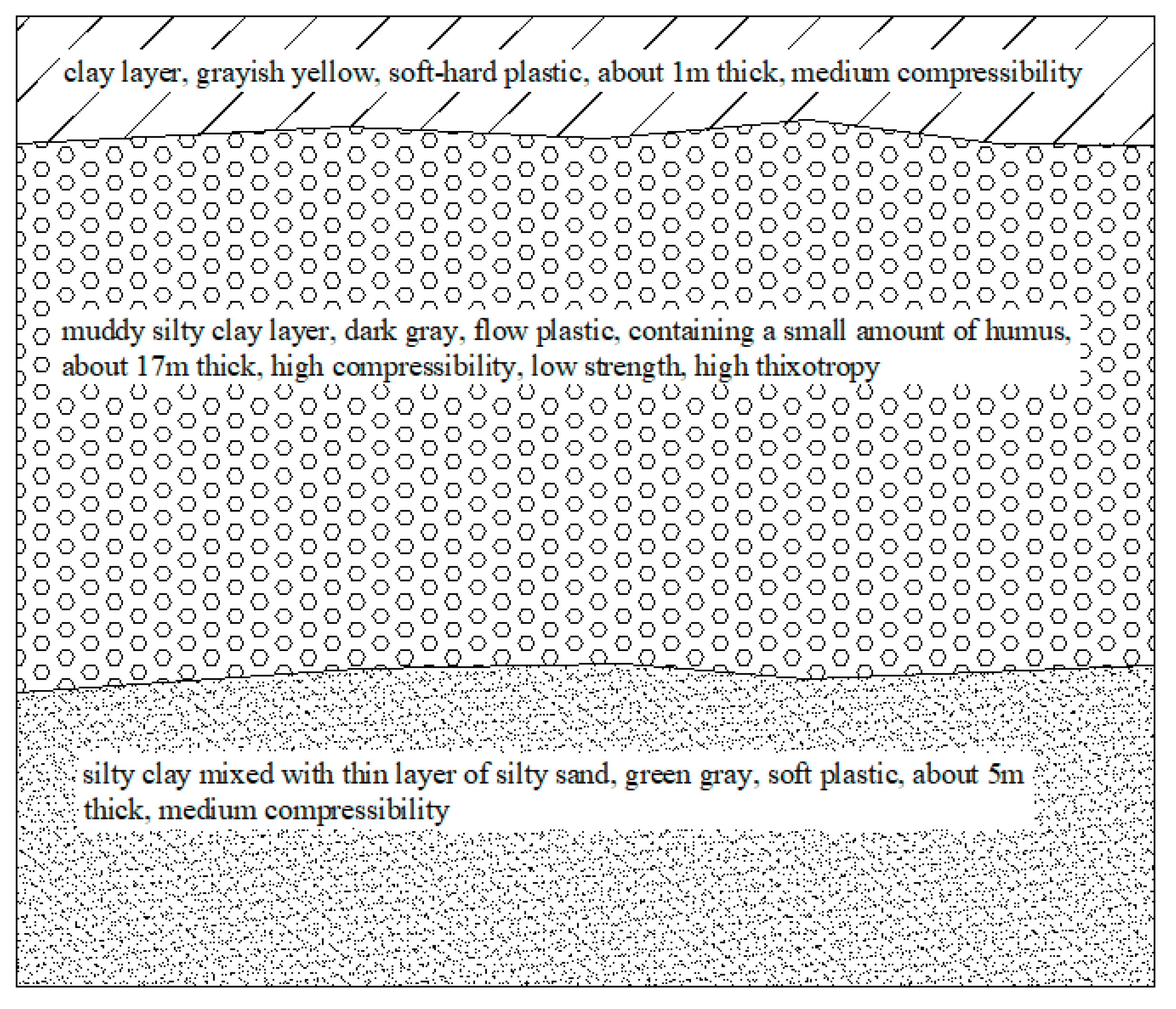
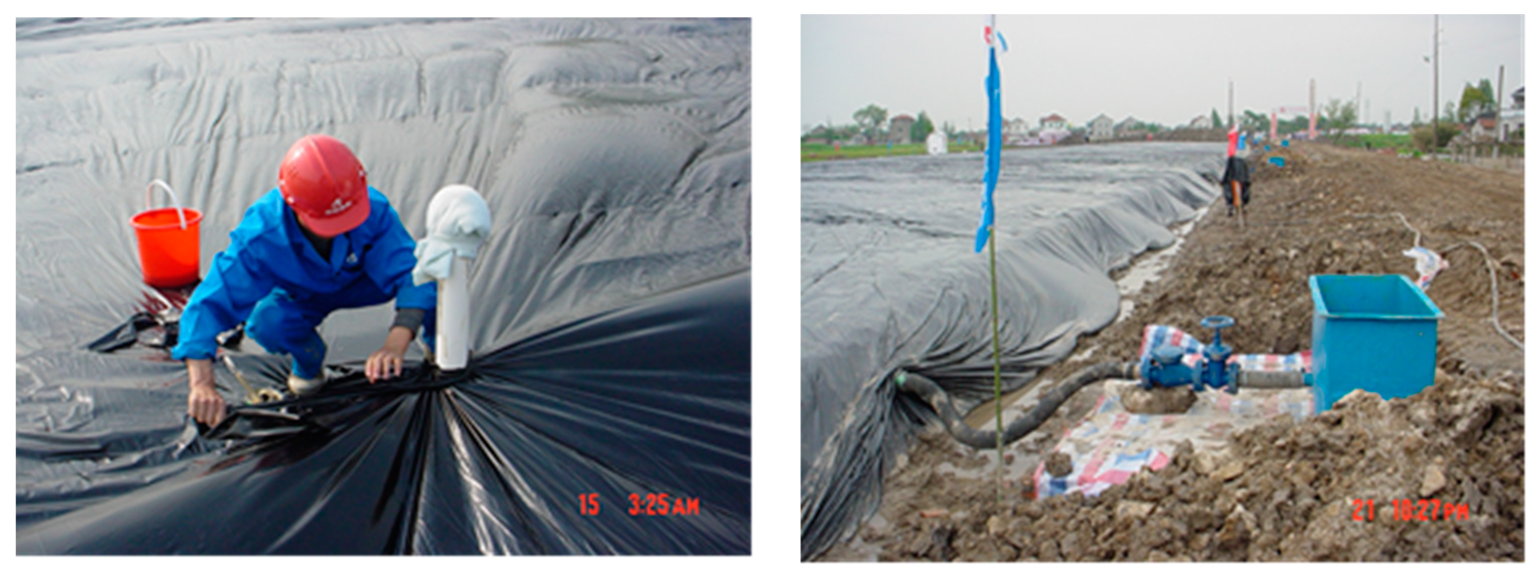
2.2. Engineering Example

In the soft foundation reinforcement test section of the Beijing–Shanghai high-speed railway, the mileage range of the soft foundation reinforced with vacuum preloading is from k0 + 276.51 to k0 + 515. In this mileage range, due to the uneven distribution of thickness of the soft soil layer, there is a range value for the depth of soft foundation reinforcement. This paper selects the soil layer distribution of the k0 + 342 section as the calculation model’s soil layer distribution. From top to bottom, there is clay with a thickness of approximately 1 m, muddy silty clay with a thickness of approximately 17 m, and silty clay with a thickness of approximately 5 m. The clay layer has medium compressibility and is hard plastic. The muddy silty clay layer is characterized by high compressibility and flow plasticity. The silty clay layer has medium compressibility and is hard plastic. The buried depth of the underground water level is 0.5~1.5 m. The geological profile is shown in Figure 1.

The Provisional Regulations on the Design of High-Speed Railway stipulated that the post-construction settlement of the embankment should be less than or equal to 10 cm, the annual settlement rate at the initial stage of completion should be less than or equal to 3 cm, and the post-construction settlement of the subgrade at the bridge–road transition section should be less than or equal to 5 cm. After comprehensive consideration and argumentation, the section from k0 + 276.51 to k0 + 515 of the route mileage range adopts the method of first vacuum and then vacuum–surcharge preloading to strengthen the soft foundation. Plastic drainage boards are arranged in a quincunx shape with a spacing of 1.2 m. After the surface of the foundation is cleaned, the sand cushion with a thickness of about 0.6 m is laid, and a layer of geogrid is laid inside it. The reinforcement depth of the soft foundation is 14.5~18.5 m. The vacuum pressure under the membrane is required to be no less than 80 kPa, and the vacuum stage lasts for 56 days. The on-site construction is shown in Figure 2.

3. Numerical Simulation Scheme

During the consolidation process, the pore water pressure of the soft foundation soil gradually decreases, the effective stress of the soil gradually increases, and the soil undergoes consolidation deformation, which is a typical manifestation of the fluid–solid coupling phenomenon. During the consolidation process of soil, there are both solid and fluid disturbances. The change in soil pore pressure causes a change in effective stress, resulting in the compression of soil volume. The volume of soil is compressed, which in turn causes the water in the soil to react with soil particles, resulting in changes in pore pressure. Therefore, the calculation of soil consolidation must consider the coupling of fluid disturbance and solid disturbance, that is, fluid–solid coupling calculation.

3.1. Seepage Model

Seepage models include isotropic seepage models, anisotropic seepage models, and impermeable material models. In fact, the soil itself has anisotropic characteristics, so it is more practical to adopt an anisotropic seepage model and set a three-dimensional permeability coefficient. The selected calculation parameters are the actual values of the undisturbed soil sampled at the site and tested, as shown in

Table 1. Calculation parameters.

Series	Clay	Smear Layer of Clay	Muddy Silty Clay	Smear Layer of Muddy Silty Clay	Silty Clay	Sand Drain
Horizontal permeability coefficient $k_{h100-200}$/cm/s	0.40 × 10−7	0.35 × 10−7	1.44 × 10−7	1.30 × 10−7	0.41 × 10−7	3 × 10−2
Vertical permeability coefficient $k_{v100-200}$/cm/s	0.52 × 10−7	0.53 × 10−7	0.68 × 10−7	0.69 × 10−7	0.57 × 10−7	3 × 10−2
Compressive Modulus $E_s$/MPa	4.61	4.61	4.35	4.35	8.77	11.66
Poisson’s ratio	0.47	0.47	0.55	0.55	0.49	0.3
Cohesion $c$/kPa	14	14	3.7	3.7	4	0
Internal friction angle $\phi$/${}^{\circ }$	15.5	15.5	18.9	18.9	26.7	36
Bulk density $\gamma$/kN·m−3	19.2	19.2	17.8	17.8	18.8	19
Water content $\omega$/%	31.9	31.9	44.4	44.4	35	/

Density of water: 1000 kg/m³, Biot modulus: 4 × 10⁹ Pa.

.

3.2. Numerical Analysis Model

The calculation grid model of a single sand-drain foundation is established below. Using the formula $r_w=\alpha \left(a+b\right)/4$ (Gao et al. [19]) ($a$ is the width of plastic drain plate, 0.1 m; $b$ is the thickness of plastic drain board, 4 × 10⁻³ m; $\alpha$ is the conversion coefficient, 2 (Holtz and Jamiolkowski [20])), the equivalent radius of the sand drain $r_w=0.05$ m is calculated. According to the literature (Dai and Gu [21], Chang et al. [22]), the radius of the affected area of the sand drain $r_e$ is 7 times the equivalent radius of the sand drain, which is 0.35 m. The radius of the smear area $r_s$ is 0.15 m, which is 3 times the equivalent radius of the sand drain. The calculation area is based on the central axis of the sand drain and is axisymmetric. The horizontal calculation range is 1.4 m, 4 times the radius of the affected area. The vertical calculation range is 23 m, including three layers, namely the clay layer, muddy silty clay layer, and silty clay layer. The entire calculation area consists of six groups: clay layer, muddy silty clay layer, silty clay layer, sand drain, smear layer of clay layer, and smear layer of muddy silty clay layer. The physical and mechanical indicators of each group are different, as shown in Table 1 and Figure 3. There are a total of 2128 elements and 2772 nodes in the calculation area, as shown in Figure 3.

3.3. Boundary and Initial Conditions

The top of the model is a free boundary; The bottom is a fixed boundary without displacement in any direction. There is vertical displacement and no horizontal displacement on the sides around the model. Each surface of the hexahedron model is a permeable boundary.

The moisture content of soft soil is very high, and the groundwater level in the test section is relatively shallow. To simplify the calculation, it is assumed that the groundwater level is flush with the ground. The pore pressure of the ground node is set to be 0, which increases linearly according to the gradient of 10 kPa. The initial stress state is the gravity field. First, the density of each group is assigned. After setting the gravity acceleration and assigning the initial stress distribution of each group, the final initial stress field distribution is calculated. After the soil mass is balanced, the deformation and node rate of the whole calculation area are assigned the value of 0.

Within 8 h after vacuuming, the vacuum under the membrane rapidly reaches around 80 kPa. Therefore, the pore pressure at the top nodes is assigned to a constant value of −80 kPa. Because the vacuum negative pressure is gradually transferred and increased from the ground down, the node in the sand-drain grouping area is set as negative pore pressure, which gradually rises from the top −80 kPa to 0, and the pore pressure increases by 4.44 kPa with each 1 m decrease in depth (the pore pressure in the middle range of the sand drain is linearly distributed, with a linear gradient of −80/18 = −4.44 kPa/m). This can be realized by programming the sub-loop command flow. The unbalance force ratio is set to 10⁻⁴. The master–slave program method is used to solve the problem. The number of mechanical sub-steps is subordinate to the number of seepage sub-steps, and the calculation time is set to 4.84 × 10⁶ s.

4. Analysis of Calculation Results

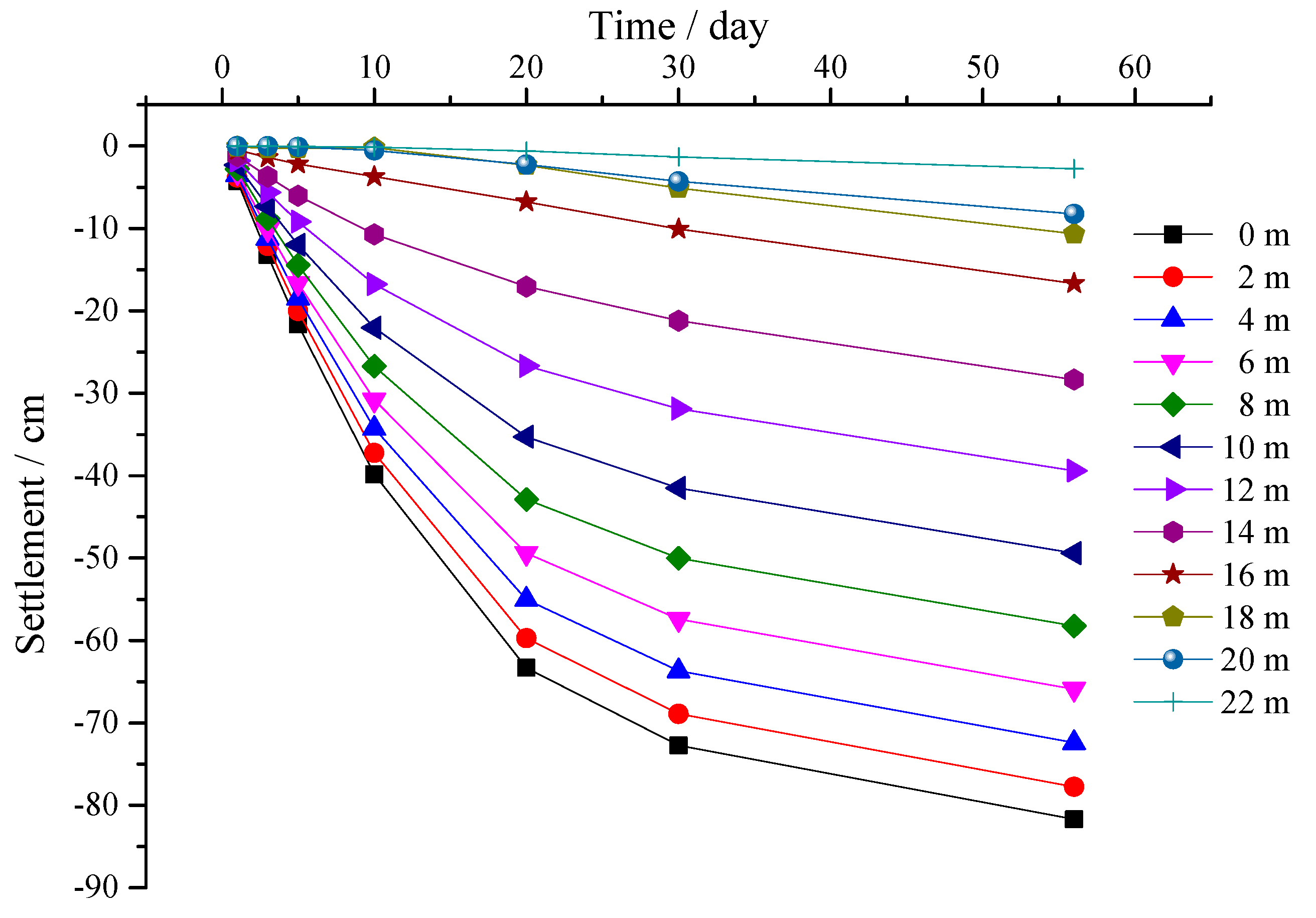
4.1. Settlement Analysis

Figure 4 shows the final vertical settlement nephogram of a single drain foundation under vacuum preloading. The settlement gradually decreases from the ground down, and the settlement is evenly distributed on the horizontal plane.

The vacuum effect is different from the surcharge effect, and its negative pressure is transferred to the sand drain quickly and then to the soil layer gradually. The soil element is subjected to isotropic pressure, so the deformation is isotropic. The macroscopic reflection is that the vertical differential settlement of each horizontal plane of the model is almost zero. Figure 5 shows the settlement curve with time at different depths at the junction of the smear layer and the soil layer. The settlement rate gradually decreases with the depth, and the settlement rate and value at the ground are the largest. At the depth of 22 m, the settlement rate and settlement value are almost 0 in the first 10 days, and there is a slight change from the 10th day, and the final value is 2.75 cm. At the depth of 18 m (at the bottom of the sand drain), the settlement rate and settlement value are almost 0 in the first 10 days, and only slightly change from the 10th day, which is more obvious than that at the depth of 22 m, reaching 10.66 cm. These results indicate that the influence range of vacuum action can basically reach the bottom of the sand drain, and the vacuum reinforcement effect is weak when the soil layer is deeper. After 30 days of vacuum action, the settlement rate at all depths decreases significantly, indicating that the soil layer gradually becomes stable. It is appropriate to set the time of vacuum preloading at 2–4 months in the project, and it is almost useless to vacuum again.

According to Terzaghi’s one-dimensional consolidation theory, the increment in pore water pressure in soil is equal to the increment in effective stress. As the pore water pressure decreases, the effective stress in the soil gradually increases, and the settlement of the soil gradually develops. The rapid decrease in pore pressure in shallow soil results in a rapid increase in effective stress, leading to significant settlement in shallow soil. The decrease in pore pressure in deep soil is relatively slow, resulting in a slow increase in effective stress, which reduces the settlement of deep soil.

Figure 6 shows the variation curve of the calculated and measured settlement values with time at the depth of 0 m and 4 m. The settlement calculation curve is relatively smooth, while the settlement measurement curve is not so smooth. The calculated value curve of settlement is in good agreement with the measured value curve, especially in the first 5 days and the last 26 days of vacuum pumping, with a large gap between 5 and 30 days. In fact, the distribution of the soil layer is not horizontal, and there is an uneven distribution phenomenon. This leads to the different transmission time and effect size of vacuum negative pressure in the soil layer and then leads to the inconsistent consolidation time and consolidation degree of the soil at the same depth. However, in the calculation, we assume that the distribution of the soil layer is horizontal, and the transmission of vacuum negative pressure in the soil layer is also stable. This leads to significant differences between the calculated curve and the mid-term measured settlement curve. As time goes on, the negative pore pressure of soil tends to be stable, and the uneven deformation of soil changes to equilibrium deformation, which gradually makes the calculated value of settlement consistent with the measured value.

The final settlement consists of instantaneous settlement, primary consolidation settlement, and secondary consolidation settlement. In this project, the secondary consolidation settlement is very small and negligible. The stress response of a soft foundation under vacuum load is different from that under surcharge, and its lateral deformation is inward contraction, and the instantaneous settlement can also be ignored. Therefore, the primary consolidation settlement of the soft foundation is the final consolidation settlement. The final consolidation settlement can be calculated using the layered summation method, and it is 72.6 cm. This is significantly different from the measured value, so it is more appropriate to use the final stable value calculated by numerical calculation as the final settlement amount.

4.2. Pore Pressure Analysis

Figure 7 shows the pore water pressure distribution nephogram of the soil model. Pore water pressure gradually increases with depth, from −80 kPa at the surface to about 168 kPa at the bottom.

The distribution of pore water pressure in the same horizontal plane within the vertical range of the sand drain is relatively uniform. At the same level, the pore water pressure in a certain range centered on the sand drain is higher than that in other locations, and there is a funnel phenomenon. The pore water pressure in the sand drain decreases the fastest under vacuum, and the pore water pressure of the soil near the sand drain decreases more than that of the soil far away from the sand drain, resulting in this funnel phenomenon. However, due to the small horizontal size of the single sand-drain foundation model, it is not very obvious.

Figure 8 shows the curve of calculated pore water pressure of soil at different depths with time. The pore water pressure of soil at different depths gradually decreases from 0, a negative value, and a positive value to a constant value, and stabilizes. The pore water pressure changes for about 30 days.

Within the first 20 days of the vacuum preloading, the pore water pressure of the soil at various depths decreased significantly. After 20 days, the pore water pressure of the soil at various depths gradually stabilized. The shallower the burial depth was, the higher the absolute value of the pore water pressure in the soil was. The deeper the burial depth was, the lower the absolute value of pore water pressure in the soil was. After the pore water pressure stabilized, the shallower the burial depth was, and the closer the pore water pressure of the soil was to the vacuum pressure under the membrane −80 kPa. In the early stage of vacuum preloading, the vacuum pressure under the membrane rapidly reached −80 kPa within 8 h. Then, the vacuum negative pressure was quickly transmitted to the sand drain and gradually transmitted to the soil. This would cause a rapid decrease in pore pressure in the soil. After the seepage of water in the soil reached equilibrium, the pore pressure of the soil at various depths would gradually stabilize. The depth of influence of vacuum preloading could be determined by the numerical value of pore pressure after the pore pressure stabilized.

The pore water pressure in soil is composed of pore water pressure formed by pressure conditions and pore water pressure formed by load action. The static water pressure below the groundwater level and the pore water pressure caused by seepage belong to the pore water pressure formed by pressure conditions. The pore water pressure formed by surcharge belongs to the pore water pressure formed by load action. In the calculation, we assumed that the groundwater level was level with the ground, and there would be static pore water pressure in the soil, which increased linearly from 0 along the depth. The vacuum action causes water to flow in the soil, and the resulting seepage force generates pore water pressure, which belongs to the pore water pressure formed by pressure conditions. In addition, the vacuum effect causes the soil to be subjected to isotropic pressure, which will generate pore water pressure formed by load action. Therefore, the variation in pore water pressure in soil under vacuum is very complex. Before applying vacuum, there is static pore water pressure in the soil. After applying vacuum, the transmission of negative pressure and the seepage of water will gradually change the pore water pressure in the soil from static pore water pressure, and the process is quite complex. Through simulation analysis, it can be concluded that the pore water pressure in the soil gradually decreases to a stable value. After seepage equilibrium, the pore water pressure in the soil at a depth of 16 m is almost zero. This indicates that there is no vacuum negative pressure effect at a depth of 16 m after 30 days, and the vacuum preloading can affect a depth of up to 16 m.

Figure 9 shows the variation curve of calculated and measured pore water pressure with time at the depths of 4 m and 6 m. The calculated curve is smooth, while the measured curve fluctuates greatly. Their changing trends are consistent.

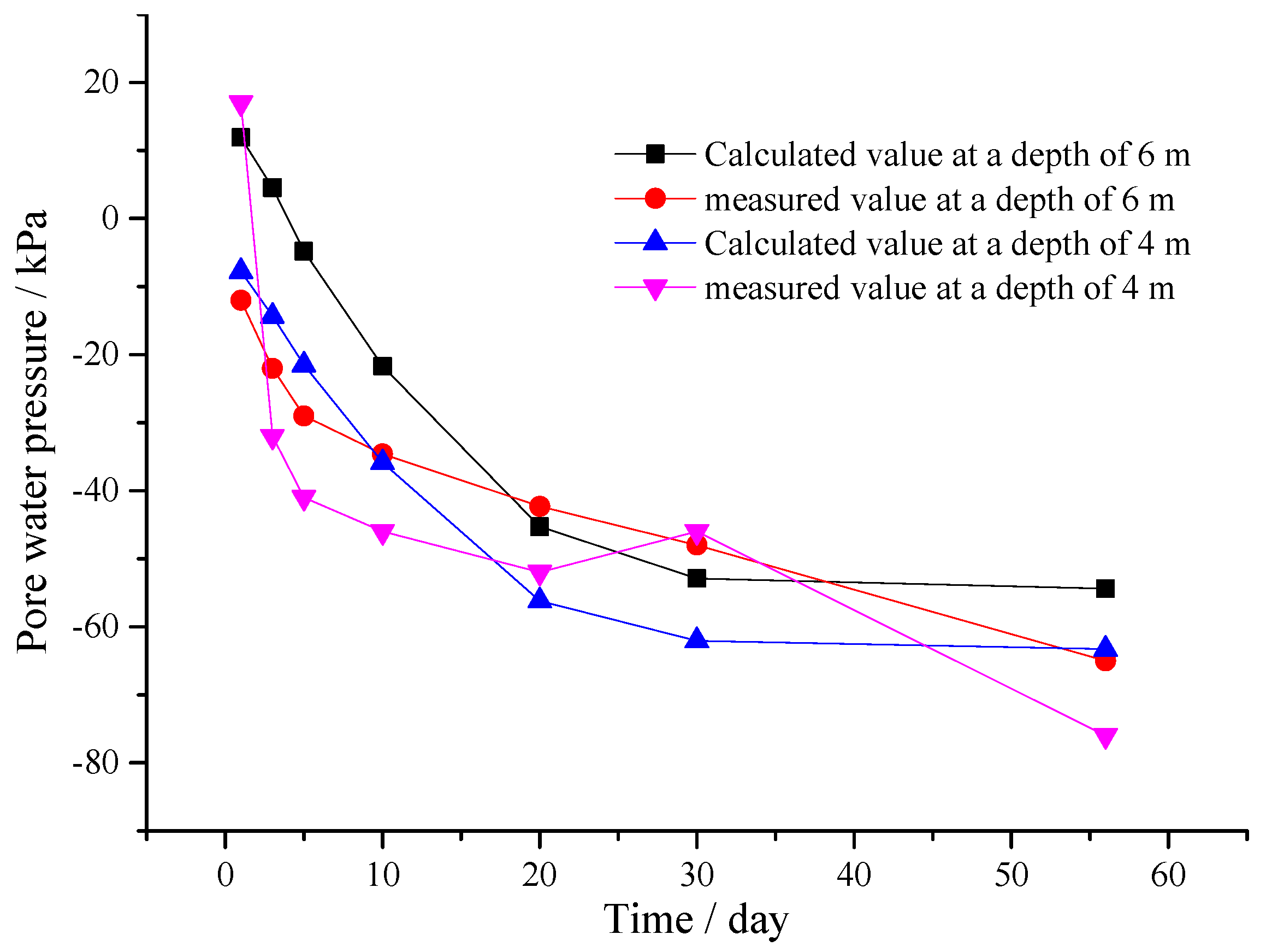
4.3. Comparison between Numerical Solution and Analytical Solution of Pore Pressure

Based on the classic consolidation equation of a single sand-drain foundation under the condition of axial symmetry and equal strain, the authors assumed the upper and lower boundaries of the foundation as semi-permeable conditions, combined them with the actual construction conditions, deduced the analytical calculation formula of pore water pressure, and calculated the analytical calculation value, as shown in Figure 10.

A paper on the analytical method was published by the Chinese journal Journal of Highway and Transportation Research and Development in April 2023. The analytical solution can be calculated according to Formula (1).

$$\stackrel{⌢}{u}=\left[{\mathrm{p}}_0\left(z\right)-u_0\left(\frac{E}{H}z-D\right)\right]e^{-\frac{E_{\mathrm{s}}}{{\gamma }_{\mathrm{w}}\mathrm{f}\left(z\right)}t}+u_0\left(\frac{E}{H}z-D\right)$$

(1)

The change trends of the analytical solution, numerical solution, and measured value are consistent. However, due to too many assumptions and simplified conditions in the derivation of the analytical formula, there is a large gap between the analytical solution curve and the measured value curve. The numerical calculation results are more consistent after 20 days of vacuum action, mainly because the vertical seepage of water in the soil is considered, and the soil layer division is more refined.

The formula for the analytical solution is quite complex. In the derivation process, we considered the reinforced soil layer as a layer of soil. Due to the presence of the sand drain, we only considered the radial seepage of water in the soil and did not consider the vertical seepage of water in the soil. In addition, the parameter calculation of the semi-permeable boundaries at the top and bottom of the soil layer had a certain degree of empiricism. Therefore, the difference between the calculated results of the analytical solution and the measured values is relatively large. However, their changing trends are basically consistent. In the future, we will further research and improve the computational accuracy of analytical solutions.

The numerical calculation results are superior to the analytical calculation results. Numerical calculations have to some extent overcome the shortcomings of the above analytical calculation methods. For example, the modeling of numerical calculations is more in line with the actual situation of soil layers; the numerical calculation considers the vertical seepage of water in the soil, and so on. However, the determination of how numerical calculation methods can improve the accuracy of results is also a process of continuous research.

The measured values are the most realistic. However, the cost of measured values is the highest. The actual measurement method also needs to be supported by actual projects. These are not easy to implement.

In summary, this analytical solution can roughly predict the trend of pore pressure changes, and numerical solutions can accurately predict the amplitude of changes in pore pressure.

5. Conclusions

Based on the principle of the finite difference method, this study used FLAC3D software to compile a command flow program for the test project of vacuum preloading soft foundation reinforcement of the Beijing–Shanghai high-speed railway, and it established a fluid–solid coupling calculation model for vacuum preloading of a single sand-drain foundation. The following conclusions were obtained after calculation:

(1)

The top surface and sand drain can be regarded as load boundary conditions for vacuum preloading to strengthen a soft foundation. The node pore water pressure at these places is assigned to a negative value, the top surface is set to a constant value of −80 kPa, and the sand drain is set to a gradient of −80 kPa to 0 kPa from top to bottom. In this way, the response of the soil consolidation process is more reasonable.

(2)

After 30 days of vacuum action, the settlement rate at all depths of the soil decreased significantly, and the soil layer gradually stabilized. It is appropriate to set the time of vacuum preloading at 2–4 months.

(3)

The transfer time and action magnitude of negative pore water pressure under vacuum are different, which makes the consolidation time and consolidation degree of soil at the same depth uneven. This is reflected in the large deviation between the measured value and the calculated value of settlement in the period of 5–30 days. However, with the extension of time, the pore water pressure in the soil tends to be stable after 30 days. At the same depth, unbalanced consolidation changes to balanced consolidation, which makes the measured value of settlement gradually consistent with the calculated value.

(4)

The change time of soil pore water pressure under vacuum is approximately 30 days. After 30 days, the pore water pressure at each depth of the soil layer tends to be stable. The influence depth of vacuum preloading can reach 16 m, and the pore water pressure of soil below 16 m is stable at a positive value.

References

1. Kjellman, W. Consolidation of clay soil by means of atmospheric pressure. In Proceedings of the Conference on Soil Stabilization; Massachusetts Institute of Technology: Cambridge, MA, USA, 1952. [Google Scholar]
2. Barron, R.A. Consolidation of fine-grained soils by drain wells. Trans. Am. Soc. Civ. Eng. 1948, 113, 718–754. [Google Scholar] [CrossRef]
3. Hansbo, S. Consolidation of fine-grained soils by prefabricated drains. In Proceedings of the 10th International Conference on Soil Mechanics and Foundation Engineering, Stockholm, Sweden, 15–19 June 1981; Volume 3, pp. 677–682. [Google Scholar]
4. Zeng, G.; Wang, T.; Gu, Y. Some Aspects of Sand-drained Ground. J. Zhejiang Univ. 1981, 1, 835–838. [Google Scholar]
5. Terzaghi, K. Theoretical Soil Mechanics; John Wiley & Sons, Inc.: New York, NY, USA, 1943. [Google Scholar]
6. Biot, M.A. General Theory of Three-Dimensional Consolidation. J. Appl. Phys. 1941, 12, 155–164. [Google Scholar] [CrossRef]
7. Hird, C.C.; Pyrah, I.C.; Russell, D. Finite element modeling of vertical drains beneath embankments on soft ground. Geotechnique 1992, 42, 499–511. [Google Scholar] [CrossRef]
8. Hird, C.C.; Pyrah, I.C.; Russel, D.; Cinicioglu, F. Modeling the effect of vertical drains in two-dimensional finite element analysis of embankments on soft ground. Can. Geotech. J. 1995, 32, 795–807. [Google Scholar] [CrossRef]
9. Indraratna, B.; Redana, I.W. Plain-strain modeling of smear effects associated with vertical drains. Geotech. Geoenviron. Engrg. 1997, 123, 474–478. [Google Scholar] [CrossRef]
10. Indraratna, B.; Redana, I.W. Numerical modeling of vertical drains with smear and well resistance installed in soft clay. Can. Geotech. J. 2000, 37, 132–145. [Google Scholar] [CrossRef]
11. Zhao, W.; Chen, Y.; Gong, Y. A methodology for modeling sand-drain ground in plain strain analysis. Shuili Xuebao 1998, 29, 54–58. [Google Scholar]
12. Zhao, Y.; Luo, S.; Wang, Y.; Wang, W.; Zhang, L.; Wan, W. Numerical Analysis of Karst Water Inrush and a Criterion for Establishing the Width of Water-resistant Rock Pillars. Mine Water Environ. 2017, 36, 508–519. [Google Scholar] [CrossRef]
13. Zhao, Y.; Liu, Q.; Zhang, C.; Liao, J.; Lin, H.; Wang, Y. Coupled seepage-damage effect in fractured rock masses: Model development and a case study. Int. J. Rock Mech. Min. Sci. 2021, 144, 104822. [Google Scholar] [CrossRef]
14. Zhao, Y.; Tang, J.; Chen, Y.; Zhang, L.; Wang, W.; Wan, W.; Liao, J. Hydromechanical coupling tests for mechanical and permeability characteristics of fractured limestone in complete stress–strain process. Environ. Earth Sci. 2017, 76, 24. [Google Scholar] [CrossRef]
15. Sha, L.; Liu, H.; Wang, G. Finite element analysis on large deformations of dredger fill improved by combined vacuum and surcharge preloading. J. Zhejiang Univ. Technol. 2021, 49, 140–146. [Google Scholar]
16. Liu, Y.; Qi, L.; Li, S.; Guo, H. 3D Finite element analysis of vacuum preloading considering inconstant well resistance and smearing effects. Rock Soil Mech. 2017, 5, 1517–1523. [Google Scholar]
17. Zhou, Q.; Zhang, H. Numerical simulation analysis and settlement calculation of vacuum combined surcharge preloading for a wharf. China Water Transp. 2018, 18, 139–143. [Google Scholar]
18. Chen, Y.; Chen, D. FLAC/FLAC3D Foundation and Engineering Example; Water Power Press: Beijing, China, 2013; Volume 6, p. 1. [Google Scholar]
19. Gao, C.-s.; Zhang, L.; Wang, Z.-j.; Wei, R.-l. Equivalent diameter of prefabricated drains. Hydro-Sci. Eng. 2002, 2002, 28–32. [Google Scholar]
20. Holtz, R.D.; Jamiolkowski, M. Prefabricated Vertical Drains: Design and Performance; Plymouth Company Ltd.: London, UK, 1991; pp. 9–56. [Google Scholar]
21. Dai, G.; Gu, H. Soil Mechanics and Foundation Engineering; Chongqing University Press: Chongqing, China, 2017; Volume 7, p. 408. [Google Scholar]
22. Chang, J.; Li, J.; Hu, H.; Qian, J.; Yu, M. Numerical Investigation of Aggregate Segregation of Superpave Gyratory Compaction and Its Influence on Mechanical Properties of Asphalt Mixtures. J. Mater. Civ. Eng. 2023, 35, 04022453. [Google Scholar] [CrossRef]
Figure 1. A picture of engineering geological sections.
Sustainability 15 07841 g001
Figure 2. Site construction.
Sustainability 15 07841 g002
Figure 3. Computation model.
Sustainability 15 07841 g003
Figure 4. Settlement nephogram.
Sustainability 15 07841 g004
Figure 5. Layered settlement–time curve.
Sustainability 15 07841 g005
Figure 6. Settlement–time curve at 0 m and 4 m depth.
Sustainability 15 07841 g006
Figure 7. Contour of pore water pressure.
Sustainability 15 07841 g007
Figure 8. Layered pore water pressure–time curve.
Sustainability 15 07841 g008
Figure 9. Pore water pressure–time change curve at 4 m and 6 m depth.
Sustainability 15 07841 g009
Figure 10. Pore water pressure–time curve at 6 m depth.
Sustainability 15 07841 g010