Environmental “Fee-to-Tax” and Heavy Pollution Enterprises to De-Capacity

Abstract

Will environmental “fee-to-tax”, which strengthens the rigidity of levies and increases the environmental costs of heavy pollution enterprises, force heavy pollution enterprises to de-capacity. This paper examines the impact and heterogeneity of the environmental “fee-to-tax” on heavy pollution enterprises’ de-capacity by taking the official implementation of the Environmental Protection Tax Law of the People’s Republic of China in 2018 as the institutional impact and the listed industrial enterprises in Shanghai and Shenzhen A-shares from 2015 to 2019 as the sample. The study found that environmental “fee-to-tax” pushed heavy pollution enterprises to de-capacity. After parallel trend tests, placebo tests, eliminate policy interference, propensity score matching, and replacement variables, the findings of this paper are robust. Further analysis shows that the effect of environmental “fee-to-tax” on heavy pollution enterprises’ de-capacity is more significant in state-owned enterprises, high financing constraints enterprises, and areas with higher tax collection and management; this effect is still effective and more significant in areas with low economic development because all environmental tax revenues are included in local finance. This paper follows up and tests the implementation effect of environmental regulations in China and provides a valuable reference for the government to promote the task of de-capacity and green transformation and upgrading of industrial structure through actively playing the role of environmental protection.

1. Introduction

Over the past 40 years of reform and opening-up, China’s economic development has achieved world-renowned successes, but the sloppy economic development model has not only increased the burden on the ecological environment, it has also made the problem of overcapacity increasingly prominent [1]. Different degrees of overcapacity are experienced by 42.8% of 35 industries [2]. Overcapacity distorts resource allocation, causes serious waste, leads to downward price movements, deteriorates enterprise performance, and reduces the overall operating efficiency of the economy. Therefore, it is a matter of deep concern for the government to make greater efforts to eliminate backward production capacity and effectively resolve the risk of overcapacity.

In recent years, the literature related to overcapacity has mainly explored the reasons for overcapacity [3,4,5,6,7,8], the formative mechanisms of overcapacity [9,10,11], consequences of de-capacity policies [12], and the factors influencing de-capacity. Regarding the pathway to de-capacity, Wang and Zheng found that enterprises’ technological innovation curbs the overcapacity problem by improving competitiveness and reducing overinvestment [13], Belke et al. argue that exports can induce firms to de-capacity [14], and Wu et al. show that strengthening the financing constraints of state-owned enterprises is conducive to forcing firms to de-capacity [15], while Lu finds that opening of high-speed rail can also induce firms to de-capacity [16], but few studies have focused on the possible impact of environmental tax policies on de-capacity of enterprises.

Previous literature has mainly examined the impact of environmental taxes on pollution control [17,18] and firm behavior. Yamazaki argues that environmental taxes can positively affect productivity by recycling tax revenues to reduce corporate income taxes [19], Liu et al. found that environmental taxes increase corporate investment in environmental protection [20], and Zhang et al. show that environmental taxes can significantly improve the quality of corporate environmental disclosure in the short term [21]. There is also a series of literature finding that environmental taxes can promote firms’ R&D innovation [22,23,24], but the impact on green innovation is uncertain [25].

In 2018, the Environmental Protection Tax Law of the People’s Republic of China was officially implemented. Compared with the Interim Measures for the Collection of Sewage Charges promulgated in 1982 and the Regulations on the Collection and Use of Sewage Charges implemented in 2003, the environmental protection tax law has undergone important changes. These changes include but are not limited to, the change from post-implementation to pre-implementation, the change from administrative to taxation, and the change from central and local sharing to full local revenue, thus improving the sewage charge system, strengthening the rigidity of the environmental “fee-to-tax” policy, and increasing the environmental costs of heavy pollution enterprises. Based on these system changes, can the environmental “fee-to-tax” force heavy pollution enterprises to de-capacity?

By selecting industrial enterprises listed in Shanghai and Shenzhen A-shares from 2015 to 2019 as a sample, and using the formal implementation of the Environmental Protection Tax Law of the People’s Republic of China in 2018 as a natural experiment, we examine the impact of the implementation of the environmental “fee-to-tax” policy on the de-capacity of heavy pollution enterprises using a difference-in-difference approach. The results show that environmental “fee-to-tax” strengthened the rigidity of the levy and increased the environmental costs of heavy pollution enterprises, thus forcing them to de-capacity, and the conclusion still holds after robustness tests such as parallel trend test, placebo test, exclusion of other policy disturbances, propensity score matching, and replacement of dependent variable. The policy is also affected by the differences in enterprises’ property rights, the degree of financing constraints, the degree of tax collection and management, and local economic development. Specifically, the pushback effect of policy implementation on heavy pollution enterprises’ de-capacity is more significant in areas with state-owned enterprises, high financing constraints enterprises, and areas with strong tax collection and management; as environmental tax revenues are fully incorporated into local finance, this effect of de-capacity is still effective in regions with low economic development.

Compared with the existing studies, there are several contributions of our study to the literature: First, this paper examines the impact of the implementation of the environmental regulation on the de-capacity of heavy pollution enterprises from the perspective of environmental “fee-to-tax”, which makes up for the shortage of environmental “fee-to-tax” in this research field. The literature has focused on the impact of environmental “fee-to-tax” on R&D innovation [20,21,22,23,24] and green innovation [25], but less on the impact on enterprises’ de-capacity. In this paper, we fill the shortage by examining the effect of environmental “fee-to-tax” on enterprises’ de-capacity. Second, this paper not only solves the possible endogeneity problem of the study by using quasi-natural experiments but also makes it possible to study the policy effect of environmental “fee-to-tax” on the de-capacity of heavy pollution enterprises more cleanly by using a difference-in-difference-in-difference approach and excluding the interference of supply-side structural reform and other environmental policies. Finally, this paper also further analyzes the heterogeneous impact of environmental “fee-to-tax” on enterprises’ de-capacity, which is of practical value. The results also show that the effect of the policy on heavy pollution enterprises’ de-capacity is more significant in state-owned enterprises, high financing constraints enterprises, areas with strong tax collection and management, and areas with low economic development. The findings of the study provide valuable theoretical applications for actively exerting the effect of the environmental “fee-to-tax” policy on de-capacity, thus promoting high-quality development of enterprises and eventually promoting the green transformation and upgrading of industrial structure in the context of the “double carbon” guidance.

The rest of the paper is organized as follows: Section 2 presents the research hypotheses through theoretical analysis based on the background of the environmental “fee-to-tax” policy; Section 3 presents the research design; Section 4 presents the empirical results and analysis; Section 5 presents the further research analysis; Section 6 presents the discussion. Finally, the conclusions and recommendations.

2. Institutional Background, Theoretical Analysis, and Hypothesis Formulation

2.1. Institutional Background

The sewage charge was first regulated by the State Council in 1982 with the issuance and implementation of the Interim Measures for the Collection and Use of Sewage Charges, and then the State Council issued and implemented the Regulations on the Collection and Use of Sewage Charges in 2003. For nearly forty years, the collection of sewage charges has greatly restrained and improved the environmental pollution problem of enterprises, but the problems of low charges and insufficient rigidity of collection have been increasingly exposed. In view of this, the Environmental Protection Tax Law of the People’s Republic of China was adopted by the Standing Committee of the Twelfth National People’s Congress of the People’s Republic of China at its 25th meeting on 25 December 2016 and has been officially implemented since 1 January 2018, which means the environmental tax replacing the sewage charge on the historical stage.

As shown in

Table 1. Table of similarities and differences between sewage charges regulation and environmental tax law.

		Sewage Charges Regulation	Environmental Tax Law
Similarities	Objectives	Protecting and improving the environment
Differences	Legislative Level	Administrative Regulations	Legal
	Collection and Management Authority	Administrative Authorities	Tax Authorities
	Revenue Attribution	Central and local government	Local government

, the environmental tax law can be seen as a continuation of the sewage charges regulation, and there are both similarities between the two, with the goal of protecting and improving the environment; but there are also differences, as follows.

First, the level of legislation rises. Sewage charges are regulated by administrative regulations, while environmental taxes are regulated by law, and the law is more effective than administrative regulations, so the rise of the legislative level can strengthen the rigidity of collection.

Second, the main body of collection and management has changed. The environmental tax is clearly based on the model of “environmental monitoring, enterprise declaration, tax collection, and information sharing”, in which the enterprises declare their emissions to the taxation department on their own initiative, and the taxation department approves the emissions and levies the tax based on the monitoring information provided by the environmental protection department. With the increasingly advanced technology of emission detection and tax collection, the information sharing and linkage between environmental protection departments and taxation departments have greatly restricted the tax evasion and leakage by enterprises and strengthened the rigidity of collection.

Third, the revenue attribution is changed. The revenue from sewage charges will be shared between the central and local governments in the ratio of 1:9, while the revenue from environmental taxes will be fully integrated into local coffers, with the central government no longer participating in the sharing. From this perspective, after the implementation of environmental “fee-to-tax”, the previously common improper intervention of local governments, such as agreed levies and arbitrary exemptions, will be improved and the rigidity of levies will be strengthened.

In summary, compared to the collection of sewage charges, the collection of environmental taxes is more compulsory, more advanced, and has more incentive to be collected. The environmental “fee-to-tax” strengthens the rigidity of environmental taxes and increases the environmental costs of enterprises, which is expected to influence their enterprises’ decisions, including the de-capacity of enterprises.

2.2. Theoretical Analysis and Hypothesis Formulation

2.2.1. Environmental “Fee-to-Tax” and Heavy Pollution Enterprises to De-Capacity

Environmental property rights have public attributes, strong externalities, and blurred property rights boundaries. In the case of defective environmental regulations, local governments will relax environmental protection standards and selectively enforce laws on emissions to attract investments, thus reducing the costs of high pollution enterprises to a certain extent, thus exacerbating the overcapacity situation of heavy pollution enterprises.

The policy of environmental “fee-to-tax” is a perfection of the sewage charges regulation, which to a certain extent clarifies the boundary of environmental property rights, strengthens the internalization of environmental costs of enterprises [26], and improves the cost of pollution governance and institutional compliance of enterprises [27,28]. The reason is that, first, the environmental “fee-to-tax” has introduced tax collection and management, strengthened the collection system, improved the collection techniques, and increased the penalties, thus reducing the tax avoidance behavior of enterprises [29,30] and improving the cost of pollution governance. Second, the environmental “fee-to-tax” has changed the tax sharing mechanism, as the central government no longer shares in environmental taxes, and all taxes are incorporated into local finance, which strengthens the match between local government’s financial and administrative powers, and under the strict constraints of the central government’s environmental performance [31], local governments will transform the regional economic development model and incorporate ecological protection awareness into policy formulation and implementation, thus strengthening the responsibility for environmental protection in the competent location, which in turn raises the cost of environmental regulation compliance for heavy pollution enterprises.

As a result, environmental “fee-to-tax” has improved the pricing mechanism of the environment as a public good, truly reflected the scarcity of environmental public goods, internalized the cost of environmental pollution, and led enterprises to make decisions based on the cost-benefit model to balance the relationship between environmental costs and benefits. This means the environmental “fee-to-tax” led enterprises to make corresponding adjustments to their product structures and management models to absorb the increased costs, forcing them to reduce the duplication of inefficient production factors and eliminate outdated production capacity. The above analysis leads to the hypothesis:

Hypothesis 1 (H1).

Environmental “fee-to-tax” force heavy pollution enterprises to de-capacity.

2.2.2. Environmental “Fee-to-Tax”, Nature of Property Rights and Heavy Pollution Enterprises to De-Capacity

Due to the political, historical, and social systems, Chinese enterprises can be divided into two categories: state-owned enterprises and private enterprises according to the nature of property rights. The public nature of state-owned enterprises and their historical missions have determined that they are different from private enterprises, which makes the implementation of environmental “fee-to-tax” policy on heavy pollution enterprises’ de-capacity influenced by the difference in property rights. Specifically, compared with private enterprises, state-owned enterprises have more social responsibility [32], which makes them more responsible for environmental protection and more affected by the environmental “fee-to-tax” policy, resulting in a pushback effect of the environmental “fee-to-tax” policy on the de-capacity of state-owned enterprises is stronger than that of private enterprises. Based on the above analysis, the second hypothesis of this paper is proposed.

Hypothesis 2 (H2).

The effect of environmental “fee-to-tax” on heavy pollution enterprises to de-capacity is more significant in state-owned enterprises.

2.2.3. Environmental “Fee-to-Tax”, Financing Constraints, and Heavy Pollution Enterprises to De-Capacity

The stronger the degree of financing constraints on enterprises, the greater the pressure to cope with the internalization of environmental costs. Therefore, when the environmental “fee-to-tax” policy is implemented, it increases the cost pressure on enterprises with strong financing constraints and makes enterprises with high financing constraints more motivated to eliminate outdated overcapacity to alleviate their already unfavorable financing environment in the face of the additional environmental costs brought by the policy, resulting in the stronger the financing constraints, the greater the effect of environmental “fee-to-tax” on enterprises to de-capacity. Based on the above analysis, the third hypothesis of this paper is proposed.

Hypothesis 3 (H3).

The effect of environmental “fee-to-tax” on heavy pollution enterprises to de-capacity is more significant in strong financing constraints enterprises.

2.2.4. Environmental “Fee-to-Tax”, Tax Collection, Management, and Heavy Pollution Enterprises to De-Capacity

By introducing the tax collection mechanism, the environmental “fee-to-tax” policy strengthens the rigidity of collection, thus reducing the degree of tax avoidance [29,30] and raising the environmental cost of enterprises, in order to balance the relationship between environmental costs and benefits pushing up by the environmental “fee-to-tax”, enterprises are forced to eliminate their inefficient factors of production. As a result, the stronger the tax collection and management, the stronger the policy effect of environmental “fee-to-tax” on heavy pollution enterprises to de-capacity. Based on the above analysis, the fourth hypothesis of this paper is proposed.

Hypothesis 4 (H4).

The effect of environmental “fee-to-tax” on heavy pollution enterprises to de-capacity is more significant in areas with strong tax collection and management.

2.2.5. Environmental “Fee-to-Tax”, Local Economic Development, and Heavy Pollution Enterprises to De-Capacity

Previous studies have found that local governments trade-off between the dual goals of economic development and environmental protection, in areas with low economic development, local governments may relax the enforcement of environmental regulations [33]. The revenues from sewage charges are shared between the central and local governments in a ratio of 1:9, while the environmental tax revenue is fully integrated into the local government and the central government no longer participates in the share. The implementation of the environmental “fee-to-tax” harmonizes the local governments’ authority and financial power in environmental protection, enhances their incentive to collect and manage environmental taxes, and inhibits their tendency to relax the enforcement of environmental regulations due to economic development, which in turn tightens the control of environmental pollution and destruction by heavy pollution enterprises in low economic development areas, which ultimately exacerbates the cost of environmental regulation compliance of heavy pollution enterprises and pushes heavy pollution enterprises to de-capacity. Based on the above analysis, the fifth hypothesis of this paper is proposed.

Hypothesis 5 (H5).

The effect of environmental “fee-to-tax” on heavy pollution enterprises to de-capacity is more significant in areas with low local economic development.

3. Research Design

3.1. Data Source and Sample Processing

The data sources of this paper are as follows: (1) sample data are obtained from China Stock Market and Accounting Research Database(https://www.gtarsc.com/, accessed on 1 April 2022) and China Research Data Service Platform (https://www.cnrds.com/Home/Index#/, accessed on 1 April 2022); (2) provincial economies data are taken from the China Statistical Yearbook and China Tax Inspection Yearbook, with both yearbooks sourced from China’s economic and social big data research platform (https://data.cnki.net/HomeNew/index, accessed on 1 April 2022).

This paper takes industrial enterprises listed in Shanghai and Shenzhen A-shares from 2015–2019 as the sample (according to the industry classification of the China Securities Regulatory Commission, enterprises in the industrial sector are those in the following industries: mining, manufacturing, electricity, heat, gas and water production, and supply). The following screening and processing of the sample and data were carried out: (1) exclude the samples of companies that were specially treated such as ST and SST, etc. (in the Chinese capital market, ST refers to the stocks of domestic listed companies that are subject to special treatment, which is also a delisting risk warning. SST refers to the company’s operating losses for two consecutive years, special treatment, and has not yet completed the share reform); (2) exclude the samples with missing variable observations and abnormal data; (3) to eliminate the influence of extreme values, this paper has carried out a 1% up and down tailing process for all continuous variables. The final sample of 8769 firm-annual observations in this paper was obtained.

3.2. Model Construction and Variable Definition

The official implementation of the Environmental Protection Tax Law of the People’s Republic of China in 2018 provides a natural experimental opportunity to explore the impact of environmental regulations on enterprises’ de-capacity, which can overcome endogeneity. To better identify the effect of the implementation of environmental “fee-to-tax” and exclude the interference of other factors in the same period, this paper distinguishes between heavy pollution enterprises and non-heavy pollution enterprises and adopts a difference-in-difference approach to construct the model to be tested, as follows:

$$\begin{array}{c}C{U}_{i,t}={\alpha }_0+{\alpha }_{1}Hp{i}_i+{\alpha }_{2}Hp{i}_i\times Tim{e}_t+{\alpha }_{3}Tim{e}_t\\ +\beta X_{i,t}+{\sigma }_t+{\phi }_r+{\epsilon }_{itr}\end{array}$$

(1)

The direct manifestation of overcapacity is the low capacity utilization of enterprises [34,35]. Therefore, if the implementation of the environmental tax policy improves the capacity utilization rate of heavy pollution enterprises, it indicates that the environmental “fee-to-tax” has forced the heavy pollution enterprises to de-capacity. Thus, in Model (1), Hpi × Time is the important variable in this paper, and its coefficient captures the average change in the capacity utilization rate of the experimental group relative to the control group during the policy period, and the hypothesis holds if the coefficient of ${\alpha }_2$ is positive.

CU is the explanatory variable to measure the capacity utilization rate of firms. Drawing on Kirkley et al. [36] and Qu [37], the stochastic frontier method is used to measure the capacity utilization rate at the micro-enterprise level using a production function beyond the logarithm, and the ratio of actual output to frontier output is used as the capacity utilization rate indicator, and the larger the indicator is, the higher the capacity utilization rate is. The specific calculation model is as follows.

$$\begin{array}{ll}ln{y}_{i,t}=a_0+& a_{1}ln{k}_{i,t}+a_{2}ln{L}_{i,t}+a_{3}t+a_4{(ln{k}_{i,t})}^2+a_5{(ln{L}_{i,t})}^2\\ & +a_6(ln{K}_{i,t})(ln{L}_{i,t})+a_7(ln{K}_{i,t})t+a_8(ln{L}_{i,t})t\\ & +a_9{t}^2+{\epsilon }_{i,t}\end{array}$$

(2)

In Model (2), $y_{i,t}$ is the actual output of firm i in year t, measured by gross operating income normalized by PPI; $k_{i,t}$ is the capital input of firm i in year t, measured by total assets normalized by fixed-asset investment index; $L_{i,t}$ is the labor input of firm i in year t, measured by the number of employees; t is the time trend term, indicating technological progress; and ${\epsilon }_{i,t}$ is the composite residual term.

Hpi denotes the experimental variable in the method. The purpose of this paper is to investigate the impact of environmental “fee to tax” on the de-capacity of heavy pollution enterprises, therefore, this paper treats heavy pollution enterprises as the experimental group and classifies other enterprises as the control group, and assigns the values of 1 and 0 respectively. In accordance with the 2008 “Listed Companies Environmental Information Disclosure Guidelines” issued by the General Office of the Ministry of Environmental Protection, combined with the China Securities Regulatory Commission’s industry classification standards in 2012, the following were selected: (1) coal mining and washing industry; (2) oil and gas mining industry; (3) ferrous metal mining and selection industry; (4) non-ferrous metal mining and selection industry; (5) non-metallic mining and selection; (6) wine, beverage and refined tea manufacturing industry; (7) textile industry; (8) leather, fur, feather and its products and footwear industry; (9) paper and paper products industry; (10) petroleum processing, coking and nuclear fuel processing industry; (11) chemical raw materials and chemical products manufacturing industry; (12) medical manufacturing industry; (13) chemical fiber manufacturing industry; (14) rubber and plastic products industry; (15) non-metallic mineral products industry; (16) ferrous metal smelting and rolling processing industry; (17) non-ferrous metal smelting and rolling processing industry; (18) metal products industry; (19) electricity, heat production and supply industry.

Time represents a time dummy variable to measure the exogenous impact of the environmental “fee-to-tax” in the method. Since the Environmental Protection Tax Law of the People’s Republic of China was formally implemented on 1 January 2018, this paper takes 2018 as the base year, and time is assigned a value of 1 if it is in 2018 and later, and 0 if it is in previous years.

Referring to the existing literature, the following control variables are selected in this paper: firm size (Size), profitability (Roa), financial leverage (Lev), growth (Grow), firm age (Age), market-to-book ratio (Pb), nature of ownership (Soe), shareholding of the first largest shareholder (Top₁), investment in fixed assets (PPE), and investment in intangible assets (INTANG). In addition, this paper controls for year fixed effects (${\sigma }_t$) and region fixed effects (${\phi }_r$). The specific variables are defined as shown in

Table 2. Variable definition table.

Variable Type	Variable Code	Variable Name	Variable Definition
Explained variables	CU	Capacity utilization rate	Ratio of actual output to frontier output measured by the stochastic frontier method
Explanatory variables	Hpi	Heavy pollution enterprises	1 if it is a heavy pollution enterprise, 0 otherwise
	Time	Policy Implementation	1 if it is in 2018 and later, and 0 otherwise
	Hpi × Time	Interaction items	Interaction items of heavy pollution enterprises and policy implementation
Control variables	Size	Firm size	Natural logarithm of total assets
	Roa	Profitability	Return on total assets, net income/total assets
	Lev	Financial leverage	Gearing ratio, total liabilities/total assets
	Grow	Growth	Operating income increase rate, (current period operating income—prior period income)/prior period income
	Age	Firm Age	Ln (current year − opening year + 1)
	Pb	Market-to-book ratio	Company market value/book value
	Soe	Nature of ownership	The actual control of the company is defined as 1 by the central or local government, otherwise it is 0
	Top1	Shareholding ratio of the first largest shareholder	Total number of shares held by the largest shareholder/Total number of shares
	PPE	Investment in fixed assets	Net fixed assets/total assets
	INTANG	Investment in intangible assets	Net intangible assets/total assets

.

4. Empirical Results and Analysis

4.1. Descriptive Statistics

Table 3. Descriptive statistics.

Variable	N	Mean	Standard Deviation	Minimum	Median	Maximum
CU	8769	0.8151	0.0741	0.4736	0.8347	0.9092
Hpi	8769	0.4280	0.4948	0.0000	0.0000	1.0000
Time	8769	0.4779	0.4995	0.0000	0.0000	1.0000
Size	8769	22.2241	1.2233	20.0648	22.0712	26.0368
Roa	8769	0.0342	0.0697	−0.3227	0.0357	0.1916
Lev	8769	0.4063	0.1930	0.0630	0.3962	0.9129
Grow	8769	0.1585	0.3487	−0.5089	0.1029	2.0106
Age	8769	2.9620	0.2571	2.3026	2.9957	3.5835
Pb	8769	2.1030	1.2946	0.8638	1.6834	8.1370
Soe	8769	0.2967	0.4568	0.0000	0.0000	1.0000
Top1	8769	34.0581	13.9249	10.0100	31.9900	71.2400
PPE	8769	0.2401	0.1451	0.0263	0.2111	0.6931
INTANG	8769	0.0481	0.0413	0.0016	0.0382	0.2622

reports the results of descriptive statistics for the variables. Among them, the mean and median values of capacity utilization rate (CU) are about 81.51% and 83.47%, respectively, and the standard deviation of the variables is 7.41%, with a maximum value of about 90.92% and a minimum value of about 47.36%, indicating that there are still large differences in the capacity utilization rates of different firms in the sample interval. the mean value of Hpi is 0.4280, indicating that about 3753 firms are in the experimental group. The rest of the control variables are largely similar to the existing literature.

4.2. Baseline Regression

Table 4. Baseline regression.

	CU
	(1)	(2)	(3)	(4)
Hpi × Time	0.0139 ***	0.0087 ***	0.0086 ***	0.0068 ***
	(5.6190)	(3.6446)	(3.6174)	(3.1341)
Hpi	−0.0125 *** (−3.4625)	−0.0084 ** (−2.3271)	−0.0083 ** (−2.3021)	0.0049 * (1.6825)
Time	0.0105 *** (6.8504)	0.0114 *** (6.7623)	0.0114 *** (4.6524)	0.0108 *** (4.7548)
Size		−0.0088 ***	−0.0089 ***	−0.0080 ***
		(−5.6431)	(−5.7084)	(−6.1717)
Roa		0.3376 *** (14.6323)	0.3376 *** (14.6278)	0.2836 *** (14.4782)
Lev		0.0651 ***	0.0650 ***	0.0661 ***
		(5.8455)	(5.8133)	(6.9547)
Grow		0.0081 ***	0.0083 ***	0.0108 ***
		(2.6877)	(2.7239)	(4.0702)
Age		0.0082	0.0080	0.0070
		(1.4781)	(1.4332)	(1.4652)
Pb		−0.0021 *	−0.0022*	−0.0013
		(−1.7525)	(−1.7823)	(−1.1456)
Soe		−0.0106 ***	−0.0105 ***	0.0062 **
		(−2.9405)	(−2.9218)	(1.9689)
Top1		0.0001	0.0001	0.0001 *
		(1.2130)	(1.2015)	(1.7309)
PPE		−0.0035	−0.0036	0.0025
		(−0.2869)	(−0.2963)	(0.2444)
INTANG		−0.1459 ***	−0.1458 ***	−0.1086 ***
		(−3.6008)	(−3.5959)	(−3.0713)
Constant	0.8126 *** (388.6267)	0.9548 ***	0.9593 ***	0.9417 ***
		(28.3714)	(28.5812)	(33.5538)
Year fixed effects	No	No	Yes	Yes
Area fixed effects	No	No	No	Yes
N	8769	8769	8769	8769
Adjusted R-squared	0.0156	0.1231	0.1236	0.3690
F-value	69.0441 ***	40.9965 ***	34.0973 ***	26.4583 ***

Note: * p < 0.1, ** p < 0.05, *** p < 0.01; t-values for clustering to the firm level are in parentheses.

reports the baseline regression results, where column 1 shows the regression results without any control variables, and Hpi × Time is 0.0139, which is significantly positive at 1%; column 2 shows the estimated coefficient of the Hpi × Time is 0.0087, which is also significantly positive at 1% when only firm-level control variables are included; In columns 3 and 4, further controlling for year and region, it is found that the estimated coefficients of Hpi × Time are 0.0086 and 0.0068, which are both significantly positive at 1%. This shows that environmental “fee-to-tax” improves the capacity utilization rate of heavy pollution enterprises, indicating that the implementation of the policy has forced heavy pollution enterprises to de-capacity, and this significant relationship is not affected by the choice of control variables. Therefore, Hypothesis 1 was verified.

The results show that the environmental “fee-to-tax” policy has pushed the heavy pollution enterprises to de-capacity. On the one hand, the introduction of a tax collection and management strengthens the rigidity of the levy and reduces the degree of tax avoidance by enterprises, thus raising the cost of pollution control. On the other hand, the environmental tax is fully owned by the local government, which strengthens the match between the local government’s financial and administrative rights in environmental protection and raises the cost of environmental regulation compliance. These institutional changes lead to the implementation of policies that enhance the internalization of environmental costs for enterprises, prompting heavy pollution enterprises to eliminate backward and ineffective production capacity to balance cost benefits.

4.3. Difference-in-Difference-in-Difference

To mitigate the bias caused by the change of regional environmental tax standards, this paper constructs the indicator UP to measure the increase or not of the regional environmental tax, based on the method of Jin et al. [38] and assigns a value of 1 if the region is a standard-raising region and 0 otherwise. As shown in

Table 5. Difference-in-Difference-in-Difference.

	CU
	(1)
Hpi × Time × UP	0.0079 *
	(1.8027)
Hpi × Time	0.0034
	(1.1621)
Hpi × UP	−0.0031
	(−0.5568)
Time × UP	−0.0031
	(−1.0744)
Hpi	0.0063 (1.6233)
Time	0.0120 *** (4.7071)
UP	0.0018
	(0.2725)
Size	−0.0080 ***
	(−6.1764)
Roa	0.2835 *** (14.4865)
Lev	0.0661 ***
	(6.9482)
Grow	0.0108 ***
	(4.0703)
Age	0.0070
	(1.4554)
Pb	−0.0013
	(−1.1477)
Soe	0.0062 **
	(1.9746)
Top1	0.0001 *
	(1.7217)
PPE	0.0024
	(0.2339)
INTANG	−0.1086 ***
	(−3.0730)
Constant	0.9416 ***
	(33.5685)
Year fixed effects	Yes
Area fixed effects	Yes
N	8769
Adjusted R-squared	0.3689
F-value	24.4428 ***

Note: * p < 0.1, ** p < 0.05, *** p < 0.01; t-values for clustering to the firm level are in parentheses.

, the estimated coefficient of Hpi × Time × UP is still significantly positive at the 10% level, indicating the effect of environmental “fee-to-tax” on the de-capacity of heavy pollution enterprises is not affected by the change of regional environmental tax. This further verifies the hypothesis of this paper.

4.4. Robustness Tests

4.4.1. Parallel Trends

In this paper, we adopt the Event Study Approach to empirically test the dynamic effects of the environmental “fee-to-tax” policy, taking the previous period as the base period to avoid multicollinearity, and the results are shown in

Table 6. Parallel trend.

	CU
	(1)
Before3	0.0050
	(1.4353)
Before2	0.0050
	(1.5243)
Current	0.0112 ***
	(4.3490)
After1	0.0120 ***
	(4.7068)
Size	−0.0080 ***
	(−6.1499)
Roa	0.2839 ***
	(14.5075)
Lev	0.0657 ***
	(6.9146)
Grow	0.0108 ***
	(4.0838)
Age	0.0072
	(1.4947)
Pb	−0.0012
	(−1.1241)
Soe	0.0062 **
	(1.9777)
Top1	0.0001 *
	(1.7267)
PPE	0.0035
	(0.3548)
INTANG	−0.1080 ***
	(−3.0586)
Constant	0.9400 ***
	(33.4730)
Year fixed effects	Yes
Area fixed effects	Yes
N	8769
Adjusted R-squared	0.3687
F-value	25.3387 ***

Note: * p < 0.1, ** p < 0.05, *** p < 0.01; t-values for clustering to the firm level are in parentheses.

and Figure 1. In Table 6, Before3 and Before2 denote the three years before and the two years before the implementation of the environmental “fee-to-tax” policy, while Current and After1 denote the year and the year after the implementation of the environmental “fee-to-tax” policy.

As shown in Table 6 and Figure 1, the estimated coefficients are not significant in the first three years (Before3) and the first two years (Before2) of the environmental “fee-to-tax” policy, indicating that there is no significant difference between the experimental group and the control group before the institutional shock, which satisfies the parallel trend hypothesis. Besides, the coefficients of Current and After1 are significant and increase after the implementation of the environmental “fee-to-tax” policy, indicating that the environmental “fee-to-tax” has pushed the heavy pollution enterprises to de-capacity and that this effect strengthens over time.

4.4.2. Placebo Test

(1) Simulation of policy timing. In this paper, we use the counterfactual method [39], to conduct a placebo test to test the effect of environmental “fee-to-tax” on the de-capacity of heavy pollution enterprises by artificially setting a time point for policy implementation, and if the coefficient is not significant, the proposition is robust, and vice versa. The results are shown in

Table 7. Placebo test.

	2015–2017 (2016)
	CU
Hpi × Time	−0.0005
	(−0.1938)
Hpi	0.0034
	(0.9220)
Time	−0.0001
	(−0.0433)
Size	−0.0107 ***
	(−6.5734)
Roa	0.3843 ***
	(12.6025)
Lev	0.0775 ***
	(6.8502)
Grow	0.0067 **
	(2.1393)
Age	0.0085
	(1.4619)
Pb	−0.0017
	(−1.3680)
Soe	0.0084 **
	(2.2617)
Top1	0.0002 **
	(2.0172)
PPE	0.0184
	(1.5771)
INTANG	−0.1198 ***
	(−2.9353)
Constant	0.9831 ***
	(27.1490)
Year fixed effects	Yes
Area fixed effects	Yes
N	4578
Adjusted R-squared	0.3622
F-value	19.0940 ***

Note: ** p < 0.05, *** p < 0.01; t-values for clustering to the firm level are in parentheses.

, with 2015–2017 as the simulated policy time interval in the table header and 2016 as the simulated implementation point of the environmental “fee-to-tax” policy in parentheses. As can be seen from Table 7, the estimated coefficient of Hpi × Time is no longer significant, and the results are robust.

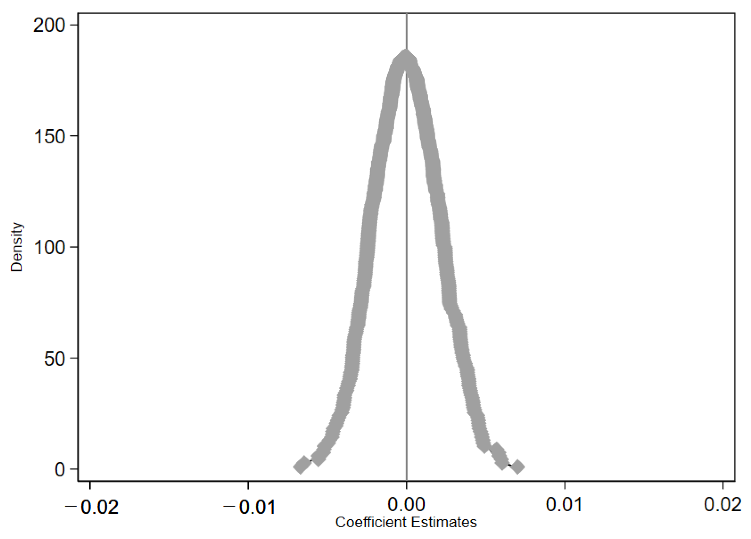
(2) Randomly simulated experimental group. Referring to the approach of Zhang et al. [40], by randomly selecting a sample comparable to the original sample experimental group as a new experimental group, the sample was repeated 800 times and baseline regression was performed based on model (1). Descriptive statistics on the estimation results showed that the mean value of the 800 estimated coefficients was −0.0000414 and the mean value of the p-value was 0.5076, which means the original hypothesis that the coefficient of the core variable in the placebo test was 0 could not be rejected. Figure 2 and Figure 3 further plot the distribution of the density and p-value of the regression coefficients, and it can be found that the estimated coefficients obtained based on the random sample are normally distributed with a mean value of approximately 0, while the true estimated coefficients in this paper (column 4 of Table 4) are clearly outliers, so the placebo test performed on the basis of the experimental group selected from the random simulation again shows robust results.

4.4.3. Exclude Other Policy Interference

To exclude the influence of other policies on the study findings, the following treatments are made in this paper. (1) To exclude the possible influence of environmental inspection (in July 2015, the 14th meeting of the Central Deep Reform Group considered and adopted the Environmental Protection Inspector Program (for Trial Implementation), which clearly established the environmental protection inspector mechanism. The Central Environmental Protection Inspectorate carried out environmental protection inspections in batches in various regions of the country during the period 2015–2018), this paper adds the dummy variable of environmental inspection (Inspection) * heavy pollution enterprises or not (Hpi) to the regression equation for control. Specifically, Inspection = 1 if the region was subjected to an environmental protection inspector in the year, and 0 in the opposite case; (2) In order to exclude possible estimation bias from carbon emissions trading and emissions trading systems (since 2011, China has been piloting a carbon emissions trading system in seven regions, including Beijing and Tianjin, etc. In 2002, China began piloting emissions trading policies in five provinces and cities, including Shandong and Shaanxi, etc. In 2007, the pilot was expanded to 11 provinces and cities, including Jiangsu, Tianjin, and Zhejiang, etc.), this paper removes the carbon emissions trading pilot region and emissions trading pilot region respectively for testing; (3) To exclude the possible role of supply-side structural reform (in 2015, the Chinese government launched the supply-side structural reform and listed “removing production capacity” as the primary task of the reform. Therefore, the State Council has introduced corresponding policy measures for overcapacity in the steel and coal industries, hoping to reduce the ineffective and low-end supply and expand the effective and mid- and high-end supply to resolve the industry overcapacity. These systems may have a certain promotion effect on the de-capacity behavior of heavy pollution enterprises), the coal and steel industries, which are deeply affected by the policy, are removed in this paper. The results are shown in

Table 8. Excluding other policy interference.

	Exclusion of Environmental Inspectors	Exclusion of Carbon Rights Pilot	Exclusion of Emissions Trading Pilot	Exclusion of Supply-Side Reform
	CU	CU	CU	CU
	(1)	(2)	(3)	(4);
Hpi × Time	0.0067 ***	0.0064 **	0.0100 ***	0.0055 **
	(3.0281)	(2.2642)	(3.3585)	(2.5156)
Hpi	0.0052 * (1.7016)	0.0043 (1.1309)	0.0005 (0.1142)	0.0063 **
				(2.1297)
Time	0.0109 *** (4.7593)	0.0115 *** (3.8126)	0.0114 *** (3.8119)	0.0107 ***
				(4.6942)
Size	−0.0080 ***	−0.0077 ***	−0.0077 ***	−0.0083 ***
	(−6.1710)	(−4.4685)	(−4.4313)	(−6.1761)
Roa	0.2836 *** (14.4786)	0.3184 *** (12.3381)	0.2826 *** (10.7774)	0.2803 ***
				(14.1709)
Lev	0.0661 ***	0.0720 ***	0.0654 ***	0.0665 ***
	(6.9550)	(6.0097)	(5.3306)	(6.9139)
Grow	0.0108 ***	0.0123 ***	0.0130 ***	0.0108 ***
	(4.0721)	(3.6066)	(3.9361)	(4.0095)
Age	0.0071	0.0079	0.0074	0.0068
	(1.4664)	(1.1907)	(1.0763)	(1.3901)
Pb	−0.0013	−0.0012	−0.0007	−0.0015
	(−1.1427)	(−1.0532)	(−0.5738)	(−1.3777)
Soe	0.0062 **	0.0055	0.0114 ***	0.0076 **
	(1.9675)	(1.3445)	(2.6460)	(2.4289)
Top1	0.0001 *	0.0001	0.0001	0.0002 **
	(1.7310)	(1.1915)	(1.1011)	(2.0582)
PPE	0.0025	0.0050	−0.0009	−0.0029
	(0.2424)	(0.3781)	(−0.0637)	(−0.2800)
INTANG	−0.1086 ***	−0.0759	−0.0685	−0.0691 *
	(−3.0719)	(−1.6088)	(−1.5065)	(−1.8997)
Inspection × Hpi	−0.0007
	(−0.4983)
Constant	0.9415 ***	0.8818 ***	0.9309 ***	0.9476 ***
	(33.5211)	(19.5198)	(24.3143)	(33.2245)
Year fixed effects	Yes	Yes	Yes	Yes
Area fixed effects	Yes	Yes	Yes	Yes
N	8769	5797	5066	8529
Adjusted R-squared	0.3689	0.3915	0.3973	0.3600
F-value	25.9095 ***	22.5330 ***	22.0883 ***	25.1704 ***

Note: * p < 0.1, ** p < 0.05, *** p < 0.01; t-values for clustering to the firm level are in parentheses.

, which shows that the coefficients of the Hpi × Time are significantly positive. This implies that competitive policies have no effect on the significance of the benchmark regression results, thus excluding the competitive hypothesis and verifying the robustness of the baseline regression results.

4.4.4. Propensity Score Matching

To mitigate the sample selection error and reduce the estimation bias of the difference-in-difference method, this paper further adopts the propensity score matching method. In this paper, we select profitability (Roa), growth (Grow), and enterprise asset level (PPE) as the characteristic variables with whether the enterprise is a heavy pollution enterprises as dummy variables, and conduct logit regression according to one-to-one matching to calculate the propensity score values, retain the samples that satisfy the common support hypothesis, and then re-test using model (1). The propensity score matching regression results are presented in

Table 9. Propensity Score Matching and Substitution of the dependent variable.

	Propensity Score Matching	Substitution of the Dependent Variable
	CU	CU1	CU2
	(1)	(2)	(3)
Hpi × Time	0.0075 *	0.0674 ***	0.2101 *
	(1.9150)	(6.5526)	(1.9254)
Hpi	0.0044	−0.0288 ** (−2.2445)	−0.0476
	(1.2402)		(−0.4623)
Time	0.0107 **	0.0339 *** (3.6384)	0.5056 ***
	(2.4359)		(4.4647)
Size	−0.0092 ***	−0.0103 *	0.0262
	(−5.5790)	(−1.6809)	(0.4677)
Roa	0.2974 ***	1.0931 *** (14.4400)	6.4465 ***
	(10.8958)		(9.0899)
Lev	0.0594 ***	0.3304 ***	2.7582 ***
	(5.1285)	(9.9450)	(8.5460)
Grow	0.0128 ***	0.0160 *	0.2291 **
	(3.2697)	(1.6856)	(2.2089)
Age	0.0027	0.0541 **	0.2675
	(0.4198)	(2.5184)	(1.2283)
Pb	−0.0022 *	0.0017	0.0989 **
	(−1.7294)	(0.4494)	(2.1286)
Soe	0.0048	0.0250 *	0.5888 ***
	(1.2653)	(1.6771)	(4.5790)
Top1	0.0001	0.0016 ***	0.0102 ***
	(0.5747)	(3.9977)	(2.7546)
PPE	0.0102	0.0088	−13.9870 ***
	(0.7515)	(0.2029)	(−30.2650)
INTANG	−0.0800 *	−0.2275 *	−9.2893 ***
	(−1.6459)	(−1.6715)	(−8.2285)
Constant	0.9782 ***	0.4387 ***	3.8646 ***
	(26.5420)	(3.1574)	(2.9531)
Year fixed effects	Yes	Yes	Yes
Area fixed effects	Yes	Yes	Yes
N	4921	8769	8769
Adjusted R-squared	0.3947	0.1430	0.3937
F-value	19.7706 ***	17.3498 ***	29.5524 ***

Note: * p < 0.1, ** p < 0.05, *** p < 0.01; t-values for clustering to the firm level are in parentheses.

column 1. As can be seen from Table 9, the estimated coefficient of Hpi × Time is significantly positive on 10% and the conclusion is robust.

4.4.5. Substitution of the Dependent Variable

In this paper, the robustness test is conducted by replacing the dependent variable. Referring to the existing literature [13,41], the total asset turnover rate CU1 (operating revenue/total assets) and the fixed asset turnover rate CU2 (operating revenue/fixed assets) are chosen to measure the capacity utilization rate, respectively, and the larger the indicator, the higher the capacity utilization rate of the firm, and the results are presented in columns 2 and 3 of Table 9. As can be seen from Table 9, the estimated coefficients of Hpi × Time are all positive at different significant levels and the conclusions are robust.

5. Further Analysis

The results of this paper show that environmental “fee-to-tax” pushes the heavy pollution enterprises to de-capacity, which supports the Hypothesis 1. To test the remaining hypotheses, this paper tests the heterogeneous performance of the reversal effect of environmental “fee-to-tax” on the de-capacity of heavy pollution enterprises by grouping according to the nature of property rights, the degree of financing constraints, the degree of tax collection and management, and the degree of regional economic development.

5.1. Environmental “Fee-to-Tax”, Nature of Property Rights and Heavy Pollution Enterprises to De-Capacity

To test the results of the reversal effect of environmental “fee-to-tax” on heavy pollution enterprises’ de-capacity under different property rights, the sample is divided into state-owned enterprises and private enterprises, and the results are reported in

Table 10. Environmental “fee-to-tax”, nature of property rights and heavy pollution enterprises to de-capacity.

	State-Owned Enterprises	Private Enterprises
	CU	CU
Hpi × Time	0.0118 ***	0.0039
	(3.2022)	(1.4474)
Hpi	0.0016 (0.2692)	0.0081 **
		(2.5608)
Time	0.0033 (0.6535)	0.0142 ***
		(5.3573)
Size	−0.0072 ***	−0.0081 ***
	(−3.4273)	(−4.9404)
Roa	0.2971 *** (7.7102)	0.2786 ***
		(12.5911)
Lev	0.0494 **	0.0717 ***
	(2.4876)	(7.0160)
Grow	0.0103 *	0.0114 ***
	(1.6474)	(4.0524)
Age	0.0073	0.0055
	(0.4798)	(1.1984)
Pb	−0.0001	−0.0015
	(−0.0188)	(−1.3445)
Top1	0.0001	0.0002 *
	(0.4830)	(1.9155)
PPE	−0.0319 *	0.0381 ***
	(−1.8415)	(3.2315)
INTANG	−0.1446 **	−0.1038 ***
	(−2.4831)	(−2.5830)
Constant	0.9665 ***	0.9302 ***
	(13.4460)	(27.7089)
Year fixed effects	Yes	Yes
Area fixed effects	Yes	Yes
N	2602	6167
Adjusted R-squared	0.3709	0.3930
F-value	10.5444 ***	18.9464 ***
Difference in coefficients between groups	0.0079 *
p-value	0.092

Note: * p < 0.1, ** p < 0.05, *** p < 0.01; t-values for clustering to the firm level are in parentheses.

.

As shown in Table 10, the estimated coefficient of Hpi × Time is significantly positive and significant at the 1% level only for state-owned enterprises, with an estimated coefficient of 0.0118, which is larger than the estimated coefficient of 0.0039 for private enterprises, and the coefficients are significantly different between groups. This indicates that state-owned enterprises have a stronger responsibility and obligation to protect the environment, resulting in a stronger pushback effect of environmental “fee-to-tax” on state-owned enterprises than private enterprises, which is in line with the goal of strengthening state-owned enterprises in the context of the “double-cycle” strategy. Thus, Hypothesis 2 is verified.

5.2. Environmental “Fee-to-Tax”, Financing Constraints and Heavy Pollution Enterprises to De-Capacity

To test the differential role of financing constraints in the effect of environmental “fee-to-tax” on heavy pollution enterprises’ de-capacity, this paper uses the SA index proposed by Hadlock and Pierce [42], SAindex = −0.737 × size + 0.043 × size2 − 0.04 × age, where the smaller the value, the lower the financing constraint on the firm and vice versa. The results are reported in

Table 11. Environmental “fee-to-tax”, financing constraints, and heavy pollution enterprises to de-capacity.

	High Financing Constraints	Low Financing Constraints
	CU	CU
Hpi × Time	0.0123 ***	0.0021
	(3.5822)	(0.7510)
Hpi	0.0001 (0.0101)	0.0088 *** (2.6612)
Time	0.0104 *** (2.7987)	0.0129 *** (4.4272)
Size	−0.0104 ***	−0.0036
	(−4.6082)	(−1.4057)
Roa	0.3597 *** (9.8390)	0.2408 *** (10.9517)
Lev	0.0793 ***	0.0559 ***
	(5.1995)	(4.8589)
Grow	0.0075 *	0.0130 ***
	(1.8245)	(3.9895)
Age	0.0157 *	0.0003
	(1.7047)	(0.0641)
Pb	−0.0009	−0.0015
	(−0.4547)	(−1.2089)
Soe	0.0040	0.0092 **
	(0.8969)	(2.2733)
Top1	0.0003 **	0.0000
	(2.4364)	(0.3641)
PPE	−0.0130	0.0236 *
	(−0.8630)	(1.7168)
INTANG	−0.1335 ***	−0.0729
	(−2.8045)	(−1.5517)
Constant	0.9671 ***	0.8630 ***
	(19.1401)	(17.5107)
Year fixed effects	Yes	Yes
Area fixed effects	Yes	Yes
N	3743	5026
Adjusted R-squared	0.3522	0.4226
F-value	13.5867 ***	22.5822 ***
Difference in coefficients between groups	0.0102 **
p-value	0.027

Note: * p < 0.1, ** p < 0.05, *** p < 0.01; t-values for clustering to the firm level are in parentheses.

.

As shown in Table 11, the estimated coefficient of Hpi × Time is positive in enterprises with strong financing constraints and significant at the 1% level, with an estimated coefficient of 0.0123, which is larger than the estimated coefficient of 0.0021 in enterprises with weak financing constraints, and the difference between the coefficients of the groups is significant. It shows that the implementation of the environmental “fee-to-tax” has raised the environmental costs of enterprises, and the effect of this increase is more significant in enterprises with high financing constraints, resulting in the implementation of the policy on heavy pollution enterprises to de-capacity is more significant in enterprises with a high degree of financing constraints. Therefore, Hypothesis 3 was verified.

5.3. Environmental “Fee-to-Tax”, Tax Collection, and Management and Heavy Pollution Enterprises to De-Capacity

To test the differential effects of the environmental “fee-to-tax” policy on the de-capacity of heavy pollution enterprises under different levels of tax collection and management. This paper refers to the measurement of tax collection and management by Sun et al. [43], and uses the ballot accuracy rate of VAT co-inspection in China Tax Inspection Yearbook to represent the tax collection and management, and divides the sample into two groups according to the mean ballot accuracy rate: regions with a high degree of tax collection and management and regions with a low degree of tax collection and management, and the results are reported in

Table 12. Environmental “fee-to-tax”, tax collection, and management, and heavy pollution enterprises to de-capacity.

	High Degree of Tax Collection and Management	Low Degree of Tax Collection and Management
	CU	CU
Hpi × Time	0.0096 **	0.0054 **
	(2.5745)	(2.0149)
Hpi	−0.0023 (−0.4732)	0.0092 ** (2.5204)
Time	0.0073 * (1.7334)	0.0126 *** (4.7077)
Size	−0.0057 **	−0.0090 ***
	(−2.3360)	(−5.7874)
Roa	0.2997 *** (8.4847)	0.2742 *** (11.5102)
Lev	0.0652 ***	0.0668 ***
	(4.1114)	(5.6035)
Grow	0.0133 ***	0.0093 ***
	(3.6244)	(2.6678)
Age	0.0073	0.0068
	(0.7741)	(1.2272)
Pb	−0.0013	−0.0011
	(−0.8207)	(−0.7967)
Soe	0.0061	0.0057
	(1.1935)	(1.4418)
Top1	0.0002	0.0001
	(1.1582)	(1.3782)
PPE	0.0054	0.0010
	(0.3124)	(0.0774)
INTANG	−0.0226	−0.1536 ***
	(−0.3575)	(−3.6918)
Constant	0.8432 ***	0.9638 ***
	(15.5286)	(28.0586)
Year fixed effects	Yes	Yes
Area fixed effects	Yes	Yes
N	3123	5646
Adjusted R-squared	0.4561	0.2993
F-value	19.5833 ***	21.3740 ***
Difference in coefficients between groups	0.0042 *
p-value	0.067

Note: * p < 0.1, ** p < 0.05, *** p < 0.01; t-values for clustering to the firm level are in parentheses.

.

As can be seen from Table 12. In columns 1 to 2, the estimated coefficient of Hpi × Time is 0.0096 and is significantly positive at the 5% level for regions with a high degree of tax collection and management, which is larger than that of 0.0054 for regions with a low degree of tax collection and management, and the difference between the two coefficients is significant. This indicates that environmental “fee-to-tax” has strengthened the tax collection and management, thus forcing the heavy pollution enterprises to de-capacity. Therefore, Hypothesis 4 was verified.

5.4. Environmental “Fee-to-Tax”, Local Economic Development, and Heavy Pollution Enterprises to De-Capacity

To test the differential impact of the environmental “fee-to-tax” on the de-capacity of heavy pollution enterprises under different levels of economic development. This paper divides the sample into two groups of high and low economic development according to the mean GDP per capita, and the results are presented in

Table 13. Environmental “fee-to-tax”, local economic development, and heavy pollution enterprises to de-capacity.

	High Degree of Economic Development	Low Degree of Economic Development
	CU	CU
Hpi × Time	0.0025	0.0122 **
	(1.1384)	(2.5499)
Hpi	0.0092 *** (3.1798)	−0.0013 (−0.2022)
Time	0.0096 *** (3.9936)	0.0118 ** (2.1954)
Size	−0.0075 ***	−0.0092 ***
	(−5.2314)	(−3.2745)
Roa	0.2391 *** (12.1210)	0.3619 *** (8.5147)
Lev	0.0652 ***	0.0706 ***
	(6.3095)	(3.5170)
Grow	0.0081 ***	0.0149 ***
	(3.2314)	(2.7224)
Age	0.0056	0.0091
	(1.2695)	(0.6953)
Pb	−0.0014	−0.0010
	(−1.0432)	(−0.4847)
Soe	0.0035	0.0097 *
	(1.0325)	(1.6896)
Top1	0.0001	0.0002
	(1.6256)	(0.9828)
PPE	−0.0013	0.0067
	(−0.1315)	(0.3322)
INTANG	−0.0795 **	−0.1564 **
	(−2.1988)	(−2.1673)
Constant	0.9367 ***	0.9160 ***
	(32.4187)	(12.8377)
Year fixed effects	Yes	Yes
Area fixed effects	Yes	Yes
N	5813	2956
Adjusted R-squared	0.2721	0.3087
F-value	22.9922 ***	11.9408 ***
Difference in coefficients between groups	−0.0097 **
p-value	0.026

Note: * p < 0.1, ** p < 0.05, *** p < 0.01; t-values for clustering to the firm level are in parentheses.

.

As shown in Table 13, the estimated coefficient of Hpi × Time is significantly positive only in the low economic development group. This indicates that the implementation of the environmental “fee-to-tax” policy has brought about more compulsory tax collection and stronger motivation for tax collection, and the change is greater and more influential in areas with lower economic development. This leads to the reversal of the effect of environmental “fee-to-tax” on heavy pollution enterprises’ de-capacity in regions with lower economic development, which verifies Hypothesis 5.

6. Discussion

Overcapacity in China is a “structural” contradiction [44], which means that overcapacity in China is prominent in industries that are dominated by heavy pollution enterprises. This means that China’s overcapacity is not only relative to the environmental carrying capacity, but also relative to the expected demand. First, in terms of environmental carrying capacity, excess capacity of heavy pollution enterprises deepens environmental pollution, such as haze, groundwater pollution, and higher carbon emissions, etc., thus reducing the carrying capacity of the environment. Second, in terms of demand expectations, the level of demand will decline in the face of many long-term problems such as the expected decline in global economic growth and aging. Therefore, the elimination of excess capacity has become imminent.

The active policy role of environmental protection tax to de-capacity is not only to eliminate the excess capacity being used, but also the unused capacity. In fact, long-term unused capacity is part of the excess capacity, although not polluting, but still generates ineffective fixed costs, thus prompting enterprises to eliminate this part of capacity first when facing strict environmental “fee-to-tax”.

So, will the de-capacity affect the future competitiveness of companies, or even China’s competitiveness, especially when demand recovers, which may lead to hindering economic development due to the inability to build new capacity in time. First, in the face of rising aging and other challenges, lower levels of demand are likely to persist for a long time, making the problem of overcapacity appear more and more serious. Second, one of the reasons for China’s overcapacity is precisely that too much reliance on a sloppy economic development model has instead reduced the potential for future economic development and hinders the development of the Chinese economy [45]. Therefore, the competitiveness of enterprises and the country can only be improved by eliminating excess capacity and prompting enterprises to shift their limited resources to more efficient industries.

The extent to which environmental “fee-to-tax” can achieve de-capacity, because the purpose of environmental protection may not be to de-capacity, but the whole range of different solutions, and in accordance with Goodhart’s law, companies will shift capacity to other areas to avoid the policy. In fact, it is the aim of the Chinese government to effectively promote the process of supply-side structural reform by actively playing the role of environmental protection in order to de-capacity, and for this reason, the Ministry of Environmental Protection also issued the Guidance on Actively Playing the Role of Environmental Protection for Supply-Side Structural Reform in 2016, and the findings of this paper not only meet the development requirements of China but also conduct more empirical and robustness tests, so it is acceptable to a certain extent. However, this still does not exclude that it is influenced by all other factors, which could be a direction for future research.

Enterprises will shift their investments to other fields because of the tax, but this is also the purpose of the environmental “fee-to-tax” to de-capacity. By strengthening the rigidity of the policy of taxation, it pushes heavy pollution enterprises to de-capacity, and to prompts enterprises to release their limited resources from excess capacity to other fields that are less affected by the environmental tax policy, such as fields that require more technological innovation, so as to achieve the purpose of the government to play an active role in environmental protection, in order to effectively promote the supply-side structural reform of the process of de-capacity, and then achieve industrial transformation and upgrading, and ultimately achieve sustainable and high-quality development of the Chinese economy.

7. Conclusions and Recommendations

Ecological civilization has become an important concept to be considered in government policy-making. In the face of weakening domestic and foreign demand expectations and an increasingly complex economic environment, it is imperative to promote the implementation of supply-side structural reform by actively playing a role in environmental protection, promoting the elimination of backward production capacity, and thus alleviating the mismatch between supply and demand, to ultimately achieve a “win-win” situation for both the environment and the economy. This has become an urgent task for China’s economic development. To this end, the government needs to develop a more effective environmental regulation system, to accelerate the transformation and upgrading of polluting enterprises and balance the relationship between the environment and the economy under the guidance of the “double-cycle” and “double carbon” strategies. The results of this paper show that environmental “fee-to-tax” strengthens the rigidity of the levy, raises the environmental costs of heavy pollution enterprises and pushes the heavy pollution enterprises to de-capacity, and the conclusion still holds after robustness tests such as parallel trend test, placebo test, exclusion of other policy disturbances, propensity score matching and replacement of dependent variable. Further studies have shown that the pushback effect of policy implementation on heavy pollution enterprises’ de-capacity is more significant in state-owned enterprises, high financing constraints enterprises, and areas with strong tax collection and management; as environmental tax revenues are fully incorporated into local finance, this effect of de-capacity is still effective in regions with low economic development.

Based on the conclusions of this paper, the following points are thus suggested.

First, strengthen the enforcement of environmental regulations. Environmental taxes and emission fees, as well as green credits and carbon credits, are all market-based environmental regulations. Compared with environmental legislation, law enforcement, inspection, and other command-and-control environmental regulations, the advantage of this type of environmental regulation is that economic instruments are used to promote rational decision-making based on cost-benefit considerations; the disadvantage is that the compulsion is relatively weak, and the behavior of enterprises is not directly prohibited but indirectly guided. If the implementation of environmental regulations is not strong enough, like the sewage charges, there are problems such as low charges and insufficient rigidity of collection, it is difficult to play its proper effect; while the environmental “fee-to-tax” to strengthen the rigidity of the levy, increasing the environmental costs of heavy pollution enterprises, is sufficient to change corporate decision-making, to force enterprises to de-capacity, so as to achieve the government’s goal of deepening supply-side structural reform to de-capacity.

Second, deepen the efficiency of environmental regulations. Market-incentivized environmental regulations often do not impose a “one-size-fits-all” ban on the target and its behavior but allow for certain differences according to their individual circumstances; however, this also leaves room for relaxing the enforcement of environmental regulations. Local governments may relax the enforcement of environmental regulations to maintain economic growth; however, the change of environmental “fee-to-tax” has changed the revenue sharing and stimulated local governments’ incentive to collect revenue, which inhibits this tendency. so, in addition to improving the system design and strengthening the system implementation, we need our government and enterprises to fundamentally change their concepts and rational behavior to reach the “win-win” goal of environmental protection and economic development.