Article

Assessing the Water-Resources Potential and Soil Erosion Hotspot Areas for Sustainable Land Management in the Gidabo Watershed, Rift Valley Lake Basin of Ethiopia

Institute of Technology, Hawassa University, Hawaasa P.O. Box 05, Ethiopia
*
Author to whom correspondence should be addressed.
Sustainability 2022, 14(9), 5262; https://doi.org/10.3390/su14095262
Submission received: 14 February 2022 / Revised: 6 April 2022 / Accepted: 7 April 2022 / Published: 27 April 2022

Abstract

:
For development of a comprehensive sediment management plan, it is crucial to categorize watersheds on the basis of soil erosion hotspot areas to extend the useful life of water bodies (e.g., Gidam reservoir). The goal of this study was to assess the surface water potential and identify erosion hotspot areas of the Gidabo watershed in Ethiopia using the Soil and Water Assessment Tool (SWAT) model. The SUFI-2 (Sequential Uncertainty Fitting Version 2) program was used to calibrate the model, and the model’s performance was evaluated. According to the catchment prioritization analysis, some of the sub-basins with similar land use, land cover, and soil type but with higher slope would generate higher sediment yield. Furthermore, the soil conservation scenarios were developed in SWAT, and the model result showed that average annual sediment yield could be reduced by the application of grassed waterway, filter strips, terracing, and contouring by 49%, 37.53%, 62.32%, and 54.6% respectively. It was concluded that sediment yield reduction by applying terracing was more effective than other conservation measures for affected sub-basins. The surface water potential of the watershed varies spatially from sub-basin to sub-basin, and the mean monthly surface water potential of the watershed is 33 million cubic meters. These findings can help decision-makers to develop appropriate strategies to minimize the erosion rate from erosion hotspot areas and to allocate the watershed water potential for different types of water demands. Strip planting, terracing, or contour farming may be necessary on chosen hotspot erosion sites to reduce the effect of slopes on surface runoff flow velocity and sediment transport capacity.

1. Introduction

Water is a vital and limited natural resource. Due to the increasing water need throughout the world, the accessibility of freshwater in numerous areas is decreasing due to the effect of the growing population, industrial development, high ET rate due to warming, and land-use land-cover changes [1]. Land-use land-cover change plays a major role in the availability of freshwater and is just one of the challenges currently facing water resources. The rapidly growing population together with the high dependence of the economy on agriculture contributes to increased demand and increased competition for inadequate water resources. Hence, quantifying the water resources and sediment yield of the basin is essential for the planning and management of available land water resources [2].
In a similar manner, estimating the sediment yields of the river basin is critical for evaluating the effectiveness of catchment management strategies in order evaluate the impacts of deposition of sediment on water bodies [3]. The shortage of information on the degree of erosion and sediment yields, as well as the transportation of fine sediment, impedes the design and application of better watershed management plans [4,5,6]. Sediment yield provides an important index of land degradation, severity, and trends, and it also reflects the characteristics of a watershed, as well as its history, development, use, and management [7,8]. As a result, it is important to estimate sediment yield because soil erosion affects the land (over time), downstream channels, and water bodies connected to the channels such as dams [9,10].
The water regime of a region can be investigated using the water balance approach for the planning and management of available resources at the watershed scale [2]. A water balance is a mass conservation application law that can be applied to a specific spatial unit. It is commonly utilized for watershed management practices because it is vital to understand the relationship between physical parameters of the watershed and hydrological components for any watershed development effort [11,12,13]. Precipitation, runoff, groundwater, evaporation, and transpiration must be used to estimate available resources, in addition to imports or exports of water from the catchment. There have been numerous computerized models developed to determine water balance.
The authors of [3] determined the water balance of the central Ethiopian Rift Valley lake using the SWAT model. Digital thematic maps, climatic parameters, and soil physical properties were used to create a SWAT model for the sub-basin. The system was calibrated and validated by comparing the river flow prediction with observed data. The authors of [2,4,8] also used an updated version of the SWAT model to forecast runoff and sediment losses from the basin. Moreover, the performance of the Arc SWAT and HEC HMS models was compared by evaluating statistical parameters at Katar River basin, and SWAT was selected as the best fit model in simulating the stream flows and sediment budget of the basin [14].
Sediment supply varies with respect to space and time as a result of its complicated interactions with many factors in the watershed [15], such as human activities, climate, land use and land cover, soil type, landscape, and drainage conditions [16]. These factors produce complications for the quantification of soil loss and are among the greatest challenges in natural resources and environmental planning [17,18]. Because of their complexity, computer simulation models that analyze all of the factors mediating soil erodibility and erosivity have been developed.
One of the physical-based computer simulation models is the Soil and Water Assessment Tool [19]. It is frequently used for erosion modeling in a variety of catchments and climates, including semiarid climates. It has been tested in many locations throughout the world. For instance, its capability was tested in sediment forecasting for the Warner Creek watershed in Maryland, and the assessment outcome revealed that yearly measured and SWAT-simulated sediment loads were in good agreement [20]. Similarly, in the Big Creek watershed of Southern Illinois, the authors of [21] calibrated daily SWAT sediment yield with observed sediment yield, concluding a reasonable sediment fit. For the Raccoon River watershed in Iowa, the authors of [22] found that the sediment loads predicted by SWAT were consistent with the sediment loads measured. This tool has also been tested and used in many regions in Africa [23,24,25,26,27,28,29,30,31] to estimate sediment yields from both gauged and ungauged watersheds, providing good results. Similarly, the SWAT model was used to forecast the amount of sediment and stream flow from gauged and ungauged river basins in Germany [32], the United States of America [33], China [34,35,36,37,38], and Jamaica [39]. Therefore, for this research, the SWAT model was selected to estimate the sediment yield and water balances of the Gidabo watershed.
Watershed management operations must be carried out inside basins to increase land productivity and lower water body siltation rates. Due to resource limitations, it is impractical to implement soil conservation measures across the entire basin at once. As a result, prioritizing intervention sites on the basis of the severity and risk of soil erosion is crucial. For example, in Ethiopia, interventions for soil conservation have been implemented since the 1970s [40]. However, these attempts failed to make a significant difference in the country’s chronic soil degradation issues [40,41,42]. Most recently, a watershed management approach was followed by Ethiopia’s government to prevent soil erosion in particular and reverse land deterioration in general [40,43]. Although significant progress has been made in halting soil erosion [41,43], the method is hampered by the lack of intervention prioritization strategies that identify locations extremely vulnerable to erosion. Today, Ethiopia is struggling with poverty. The implementation of irrigation by constructing water storage dams is the main approach to reducing poverty by increasing productivity. However, our dams are facing a serious problem with sedimentation. Thus, effective modeling of sediment yield and accurate determination of the water potential of the basin are crucial steps for developing watershed management plans. The Gidabo river basin is a central highland basin in Ethiopia’s Rift Valley Region, where soil erosion is widespread [44]. To address this, it is necessary to identify the basin’s most erosion-prone locations so that effective conservation measures can be implemented.
To achieve the overall goal of the study, the following objectives were addressed:
  • To estimate the current water budget of the Gidabo watershed;
  • To identify and prioritize erosion hotspot sub-catchments on the basis of estimated runoff and sediment yield;
  • To propose appropriate watershed management possibilities for reducing soil degradation complications.

2. Materials and Methods

2.1. Description of Study Area

2.1.1. Location and Topography

The Gidabo watershed is situated in the Rift Valley Basin of Ethiopia between 6°20′ and 7° N and between 38°05′ and 38°38′ E (Figure 1) with a coverage area of 3386 square kilometers.
The altitude of the catchment area ranges from 1183 to 3182 m above mean sea level (a.m.s.l). The major physiographic units in this area are undulating plains, valleys, steep stream banks, and major escarpments in the eastern region of the watershed.

2.1.2. Climate

There are rainy and dry seasons in the Gidabo watershed. The main rainy season is from April to October with a peak rainy season from April to May and a second peak rainy season from September to October. The mean monthly rainfall of the watershed varies between 37 mm and 188 mm, and the mean annual rainfall varies from 1219 mm to 1593 mm (Figure 2). The monthly average maximum temperature of the watershed varies between 24.2 °C and 33.06 °C; similarly, the average monthly minimum temperature of the watershed varies between 10.7 °C and 17.43 °C.

2.1.3. Land Use and Land Cover

Agriculture is the dominant land-use type inside the basin (Figure 3a). The entire basin is home to comprehensive farming practices, and various crops are grown during the two known rainy seasons, locally named Kiremt (June to September) and Belgi (February to May in Ethiopia). An assessment conducted by Ethiopia [44] indicated dynamic land-use and land-cover changes inside the watershed. The assessment reported the presence of comprehensive farming systems extending to peripheral lands, suffering from weak agricultural technology together with poor catchment management. This leads to the occurrence of high-degree soil erosion, a decrease in soil fertility, and land degradation as a whole.

2.1.4. Soil and Geology

The dominant soil in the watershed includes Eutric Vertisols with sandy loam in the middle sub-basin, Orthic Luvisols and Chromic Luvisols with clay to sandy loam in the upper sub-basin, Pellic Vertisols, Dystric Nitosols, and Eutric Cambisols in the upper and middle sub-basins [44] (Figure 3b). Geologically, the southern region predominantly features volcanic quaternary rhyolites and trachyte, while the western region features Oligocene to Miocene basalts. The lowlands of the watershed are covered with Holocene alluvial and Eolian deposits of Rift Valley [44].

2.1.5. Hydrology

The Gidabo basin with a total area of 3384 square kilometers is located in the Rift Valley Lake basin, particularly in the Abaya Lake sub-basin. The river is composed of various streams initiating from the highland regions of the basin. The river flows from the northeast and crosses the highway of Addis Abeba to Dilla at Aposto Town where it is gauged. The average flow of the river at the Aposto station is 17.35 m3/s [44].

2.2. River Basin Water Balance

Water balance is the driving force behind all processes in the Soil and Water Assessment Tool (SWAT) model [45]. SWAT simulates the hydrologic cycle as a function of the principle of water balance [46].
SW t = SW o + i = 1 t ( R day Q surf E a W s e e p Q g w ) ,
where SW t is the soil water content (mm), SW o is the initial water content, t is the time in (days), R day . is the rainfall amount on day I (mm), Q surf . is the surface runoff quantity on day I (mm), E a is the evapotranspiration amount on day I (mm), W s e e p . is the quantity of water entering the groundwater from the soil on day I (mm), and Q g w is the quantity of return flow on day I (mm).
In the watershed, the SWAT model simulates runoff using the curve number method of the Soil Conservation Service (SCS) [47]. It estimates the surface runoff using the following equation:
Q surf = ( R day   I a ) 2 ( R day   I a +   S ) ,
where Q surf is the accumulated runoff or rainfall excess (mm), R day is the daily rainfall depth (mm water), I a is the initial abstraction before the runoff event (mm water), and S is the retention parameter (mm water).
The variation in land surface features such as land use, slope, and management measures causes spatial variation in retention parameters. This can be expressed mathematically as
S = 2.54 × ( 1000 CN 10 ) ,
where CN is the daily curve number, which is governed mainly by land use, soil permeability, and a hydraulic group of soils. The initial abstraction I a is mostly taken as 0.2 S, and Equation (2) can be derived as
Q surf = ( R day 0.2   S ) 2 ( R day 0.8   S ) .
The SWAT model predicts the retention parameter with the help of two methods; the first method of calculation uses the soil moisture content in its profile, in which runoff is overestimated in shallow soil. CN is mainly governed by the antecedent climate, and the value is rarely governed by the soil storage. The CN estimation is based on evapotranspiration. The other method predicts the retention parameter using the accumulated plant evapotranspiration.
S = S max × ( 1 SW ( SW + exp ( W 1 W 2 + SW ) ) ) ,
where S is the retention parameter for a specified day (mm), Smax is the maximum retention parameter on any specified day (mm), SW is the moisture content of the soil excluding the water held at wilting point (mm), and w1 and w2 are shape coefficients.
When evapotranspiration governs the retention parameter, the result of the retention parameter at the end of the day can be updated as
S = S prev + E o * exp ( cncoef S prev S max ) R day Q surf ,
where S is the retention parameter for a given day (mm), Sprev is the previous day’s retention parameter (mm), Eo is the daily potential evapotranspiration (mm per day), cncoef is the average coefficient to estimate the retention coefficient for the daily curve number predictions, Smax is the daily higher retention parameter value (mm), Rday is the daily rainfall depth (mm), and Qsurf is the surface runoff (mm).
Evapotranspiration (PET) is one of the parameters for studying the water balance. In the SWAT model, three evapotranspiration prediction methods (the Penman–Monteith method [48], the Priestley–Taylor method [49], and the Hargreaves method [50]) are integrated.
The Penman–Monteith method requires solar radiation, air temperature, relative humidity, and wind sped; the Priestley-Taylor method requires solar radiation, air temperature, and relative humidity; the Hargreaves method requires air temperature only. For this study, the Penman–Monteith method was used to estimate evapotranspiration.
The Penman–Monteith equation that estimates evapotranspiration is as follows:
ET = 0.408 ( R n e t G ) + 𝛾 900 ( T + 273 ) U ( e s e a ) Δ + 𝛾 ( 1 + 0.34 U ) ,
where ET is the daily reference crop evapotranspiration (mm·day−1), R n e t is the net radiation flux (MJ·m−2·day−1), G is the heat flux density in the soil (which is very small and can be neglected) (MJ·m−2·day−1), T is the mean daily air temperature (°C), 𝛾 is the psychometric constant (kPa·°C−1), U . is the wind speed measured at 2 m height (m·s−1), e s is the saturation vapor pressure ( e a = e s × RH/100 (kPa)), RH is the relative humidity (%), and Δ . is the slope of the saturation vapor pressure curve (a·°C−1).
In a similar manner, the model estimates the ground water flow using Equation (8).
a q s h , i = a q s h , i 1 + W r c h r g Q r e v a p   W d e e p   W p u m p , s h ,
where a q s h , i is the water accumulated in the shallow aquifer on day I (mm),   a q s h , i 1 . is the water accumulated in the shallow aquifer on the previous day (mm), W r c h r g is the recharge percolating to the aquifer on day I (mm), Q r e v a p is the water entering into the soil zone on day I (mm), W d e e p is the water percolating from the shallow to the deep aquifer on day I (mm), and W p u m p , s h is the water removed from the shallow aquifer by pumping on day I (mm).

2.3. Sediment Balance

SWAT predicts soil erosion and sedimentation by applying the Modified Universal Soil Loss Equation (MUSLE) [51]. In MUSLE, the rainfall energy factor used for USLE is replaced with a runoff factor to improve the sediment yield prediction, which eliminates the need for delivery ratios and allows the equation to be applied to individual storm events. Delivery ratios are not needed with MUSLE because the runoff factor represents energy used in detaching and transporting sediment.
S e d = 11.8 × ( Q s u r f × Q p e a k × a r e a h r u ) 0.56 × K U S L E × C U S L E × P U S L E × L S U S L E × C F R G ,
where S e d is the sediment yield on a given day (metric tons), Q s u r f is the surface runoff volume (mm /ha), Q p e a k is the peak runoff rate (m3/s), a r e a h r u is the area of the HRU (ha), K U S L E is the soil erodibility factor, C U S L E is the cover and management factor, P U S L E is the support practice factor, L S U S L E is the topographic factor, C F R G is the coarse fragment factor, and 0.56 is the delivery ratio.
SWAT simulates the sediment flow in channel networks using the following formula [52]:
S e d c h = S e d c h , i S e d d e p + S e d d e g ,
where S e d c h is the suspended sediment available in the reach, S e d c h , i is the suspended sediment provided in the reach at the beginning of the time period, S e d d e p is the deposited sediment in the reach segment, and S e d d e g is sediment amount reentering the reach segment.
According to [52], SWAT simulates the quantity of sediment moved out of the channel as follows:
S e d o u t = S e d c h × V o u t V c h ,
where S e d o u t is the amount of sediment moved out of the channel, S e d c h is the suspended sediment available in the reach, V o u t is the outflow volume, and V c h is the volume in the reach segment.

2.4. Model Development and Input Description

Two datasets describing watershed features and meteorological data are required to develop the SWAT model.
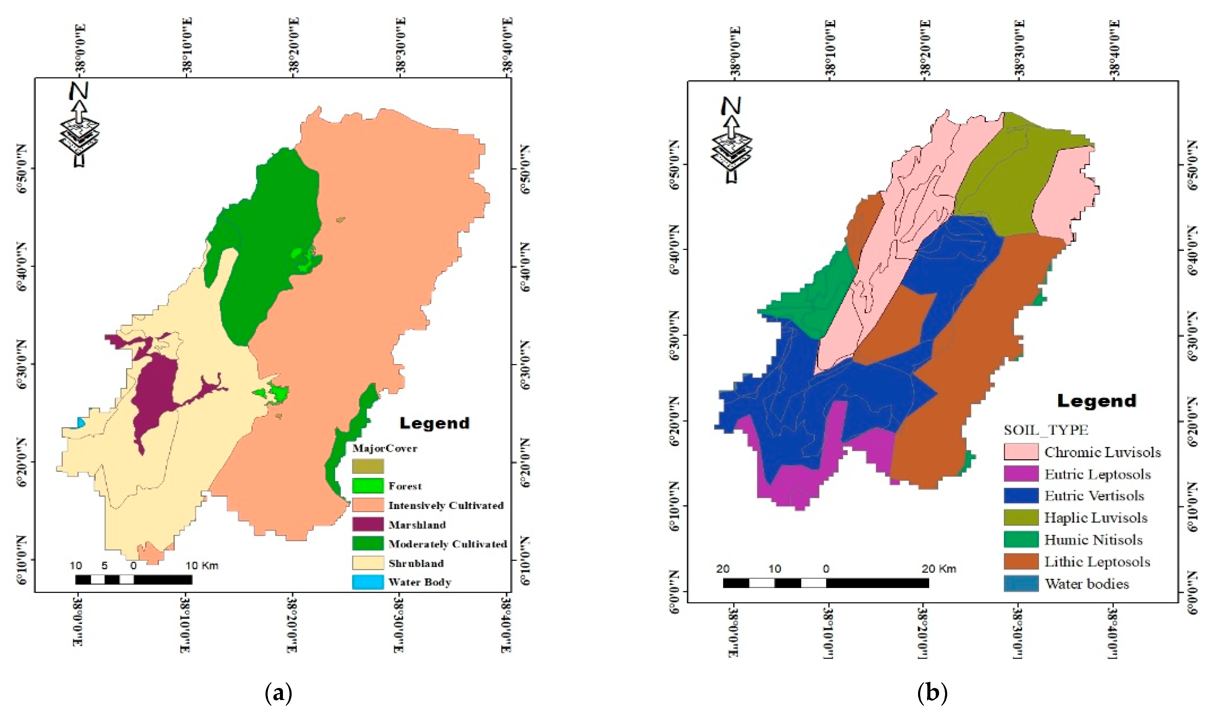
Land-use/cover data were obtained from Landsat-8 OLI (Operational Land Imager); for this study, Landsat-8 images from 2015 were used for land-use/cover classification. The satellite images of the watershed with high resolution and zero cloud cover were collected from the US Geological Survey (USGS) Center for Earth Resources Observation and Science (EROS) via https://earthexplorer.usgs.gov (accessed on 5 January 2015). ERDAS IMAGINE was used for image classification purposes, and Arc GIS10.3 was used for mapping purposes.
In the processes of image classification, the main task is assigning pixels of a constant raster images to the predefined land-cover classes. In this study, supervised classification was applied. This is the most common type of classification method in which all pixels with comparable spectral values are automatically categorized into land-cover classes. Supervised classification, which depends on the prior knowledge of pattern recognition of the research area, was used. For this study, the land-cover map was produced depending on the pixel-based supervised classification. For the land-use/cover classification, a general correctness assessment and kappa coefficient of 95.7% and 0.9402, respectively, were realized, in agreement with the minimum accuracy level (85%) recommended by [53].
The essential soil properties needed to set up the Soil and Water Assessment Tool Model are soil texture, size percentage, soil saturated hydraulic conductivity, grain, bulk density, texture class, and soil available water. These soil characteristics were obtained from laboratory analysis presented in the Rift Valley Lake Basin Master Plan study document [44]. During the study of the Ethiopian Rift Valley Lake Basin Master Plan, soil samples were collected from all soil units of the basin, and physical and chemical laboratory analyses were conducted in the Ethiopia Water Works Design and Supervision Enterprise (WWDSE) laboratory. From 13 soil units in the basin, 203 soil samples were collected, and their physical and chemical properties were analyzed. Hence, the soil database of the SWAT model was set up for the basin using the analyzed soil properties. The basin’s soil erodibility (K) factor was calculated using the equation shown in EPIC [54] from the analyzed soil parameters.
The meteorological data included daily precipitation, maximum and minimum temperature, daily wind speed, daily sunshine hours, and daily relative humidity, which were obtained from meteorological stations (Table 1) available within and nearby the study area. Daily data over 27 years (1991–2017) were collected for the study.
To fill the missing values of climate elements, a weather generator model was used. The required statistical parameters were computed using the computer program developed by [55]. As shown in Table 1, in the river basin, only one meteorological station (Dilla) was used to establish the weather generator database.

2.5. The Hydrological Data

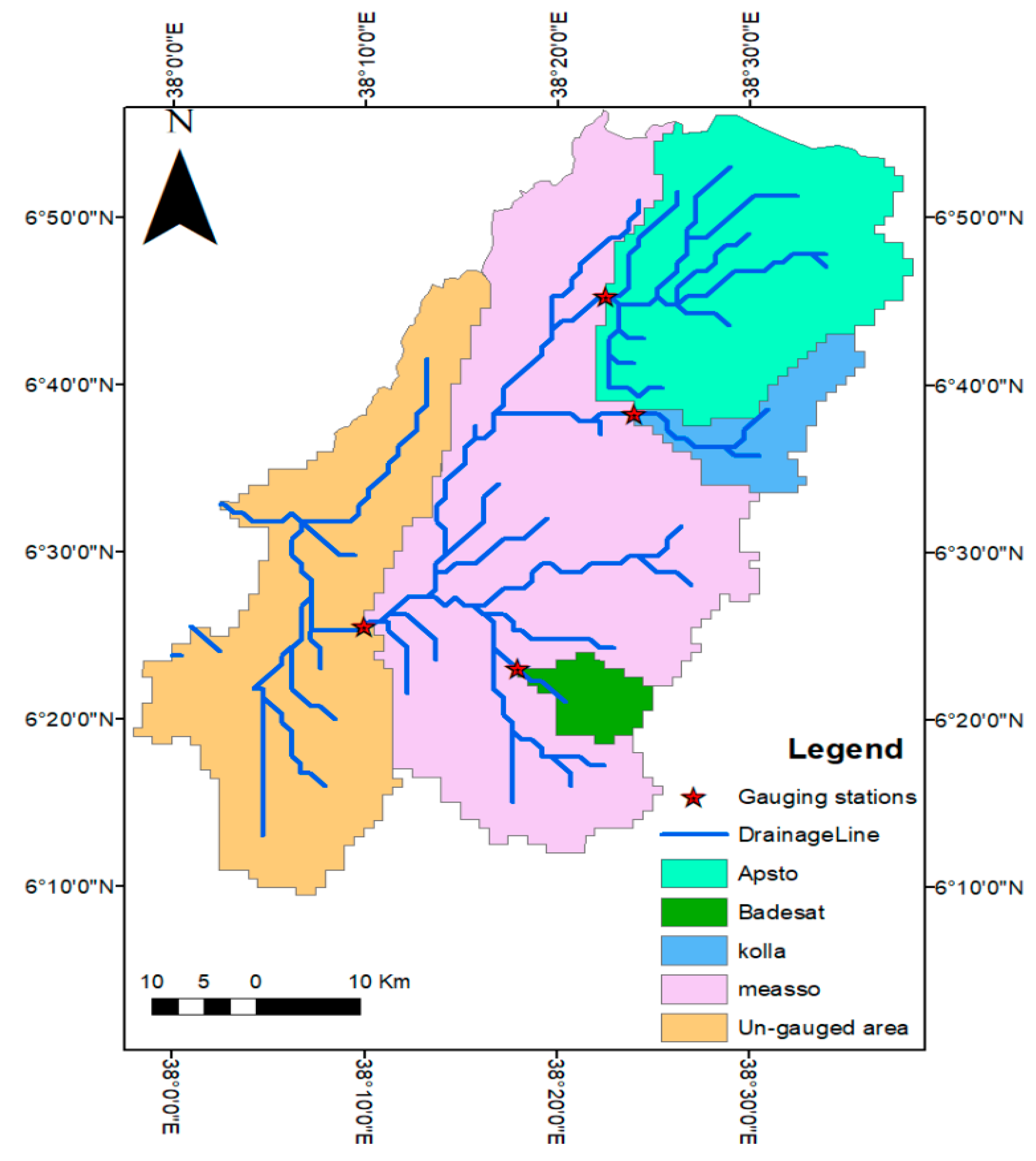
In the Gidabo river basin (total area of 3386 square kilometers), there are four stream gauging stations, namely, Aposto (area of 703 square kilometers), Kola (area of 145 square kilometers), Badessa (area of 76 square kilometers), and Measso (area of 2462 square kilometers) with data periods of 1997–2015 for Aposto, Kolla, and Badessa, whereas Measso has stream flow data from 1997–2006. As shown in Figure 4, the gauging station Measso is located near to the outlet of the watershed, and it was selected for model calibration and validation. The daily flow data of all stations were collected from the Ministry of Water and Energy of Ethiopia. For all stations (except Measso), daily flow data were available up the year 2015, and a regression model (r2 = 0.85) was used to generate the data of Measso from its upper station Aposto.
As shown in the 
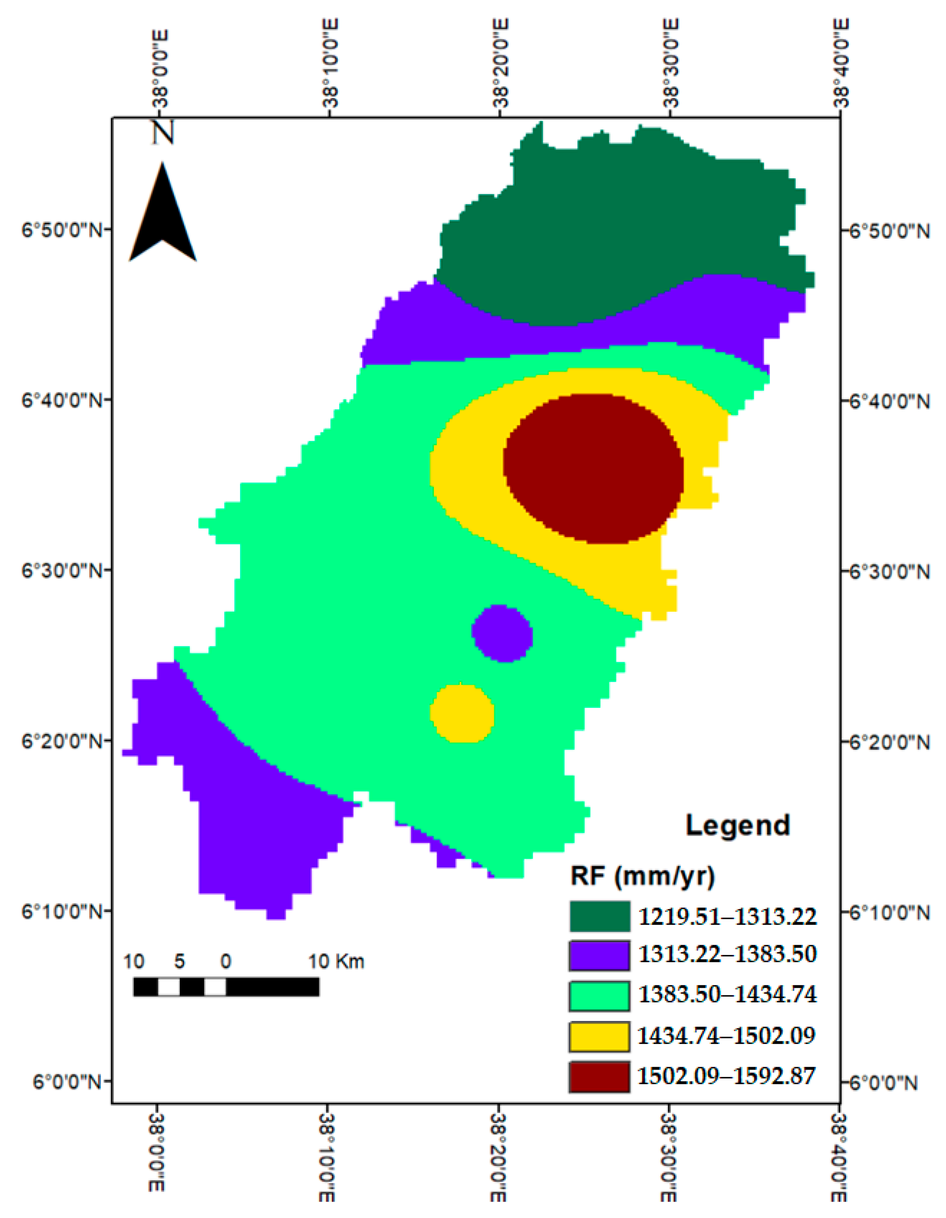
Figure 4, 27.3% of the catchment was ungauged. To predict the water and sediment budget of the ungauged regions, an empirical regression model relating sediment yield and flow of the gauged stations to several catchment characteristics, namely, drainage area, slope, and average annual rainfall, was used. Three explanatory factors were calculated for gauged and ungauged river catchments, i.e., areas of catchments and slopes were processed from the digital elevation model (DEM), and their mean annual area rainfall was calculated on the basis of the inverse distance-weighted interpolation (IDW) of the nearby meteorological stations (Figure 2).

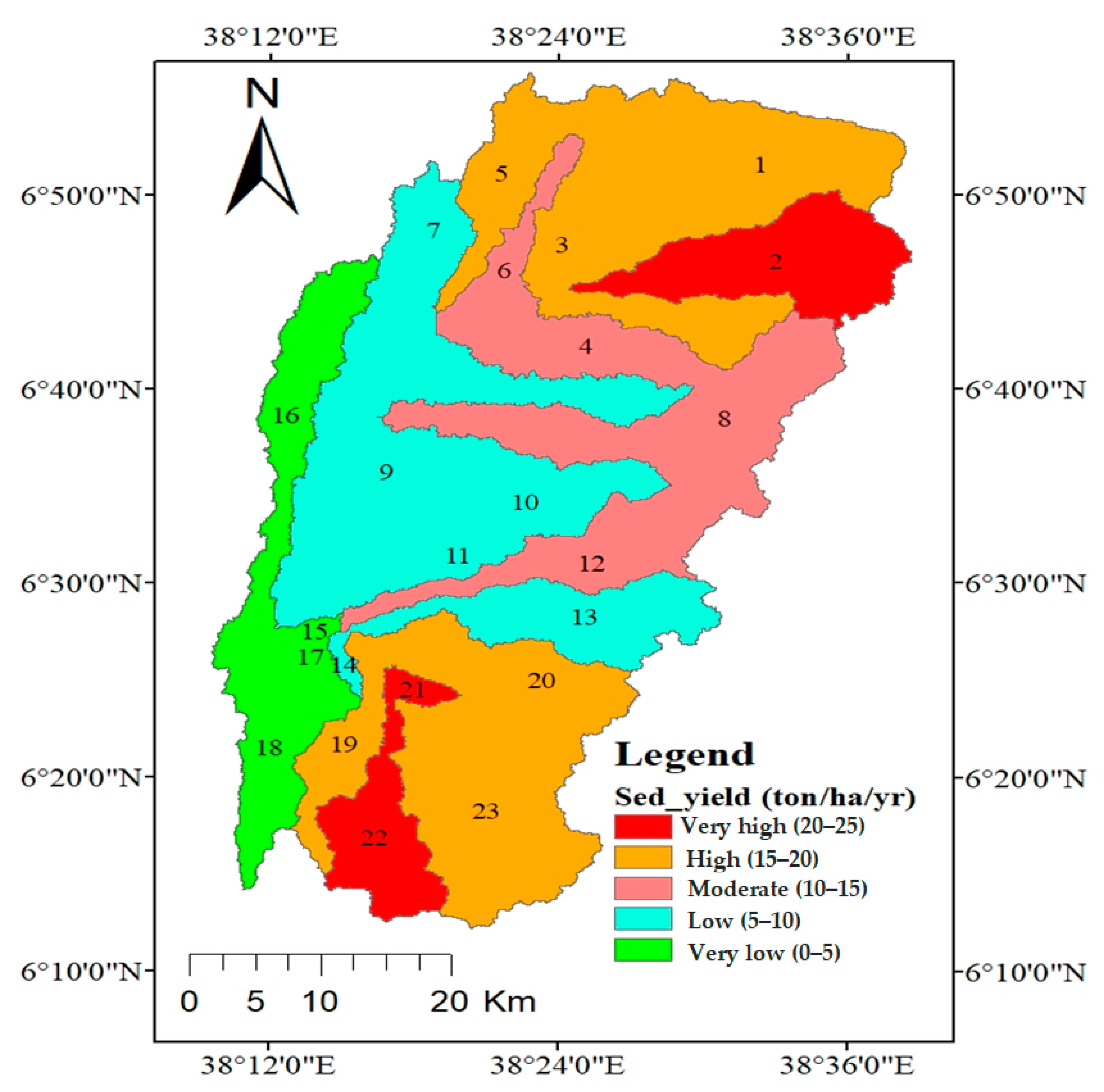
2.6. Sub-Catchment Delineation

Using the 30 × 30 m resolution DEM data, the contributing upstream area was delineated using ArcGIS 10.3 (Esri, Redlands, CA, USA). Accordingly, the entire study area was divided into 23 sub-watersheds. According to the model setup, the lowest area threshold values for land use, soil, and slope were set as 5%, 10%, and 10%, respectively, and 105 hydrological response units (HRUs) were identified, denoting unique combinations of land use, soil type, and slope.

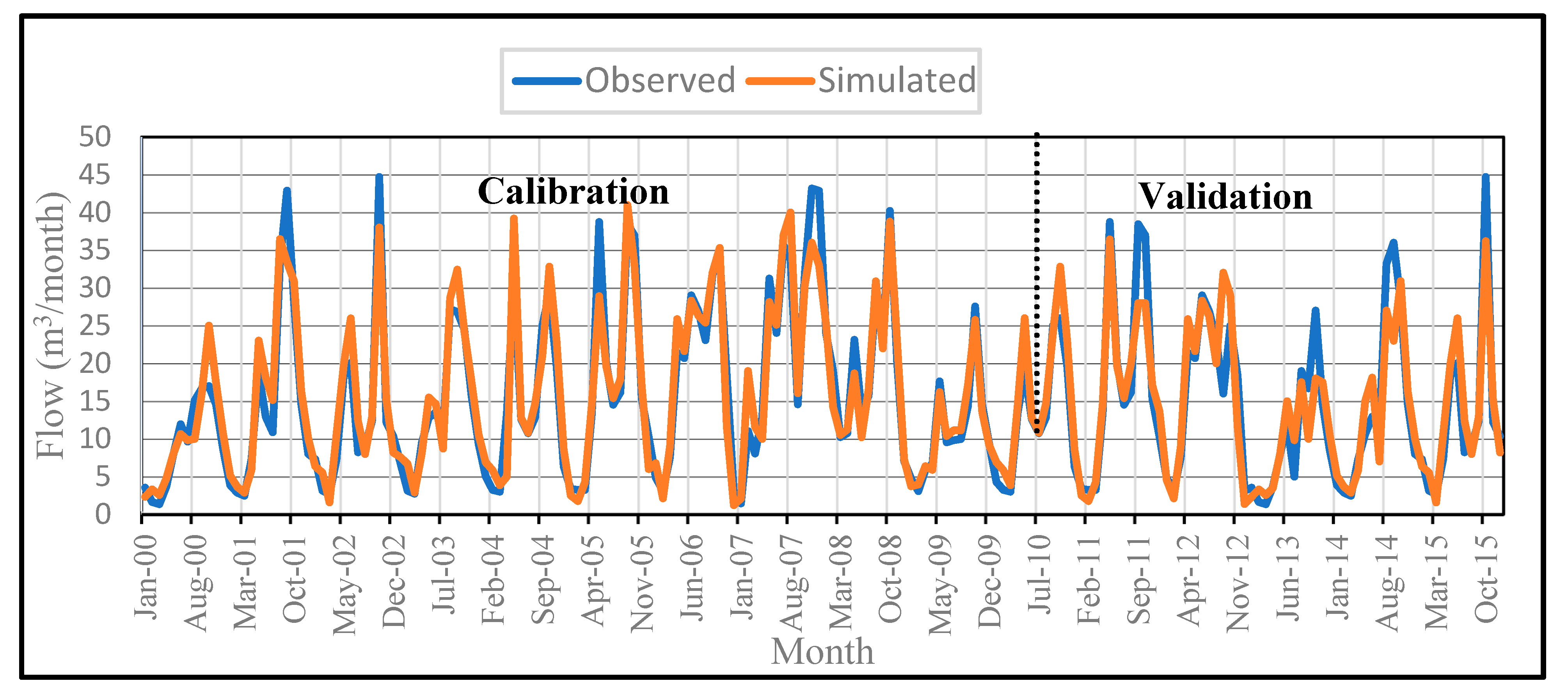
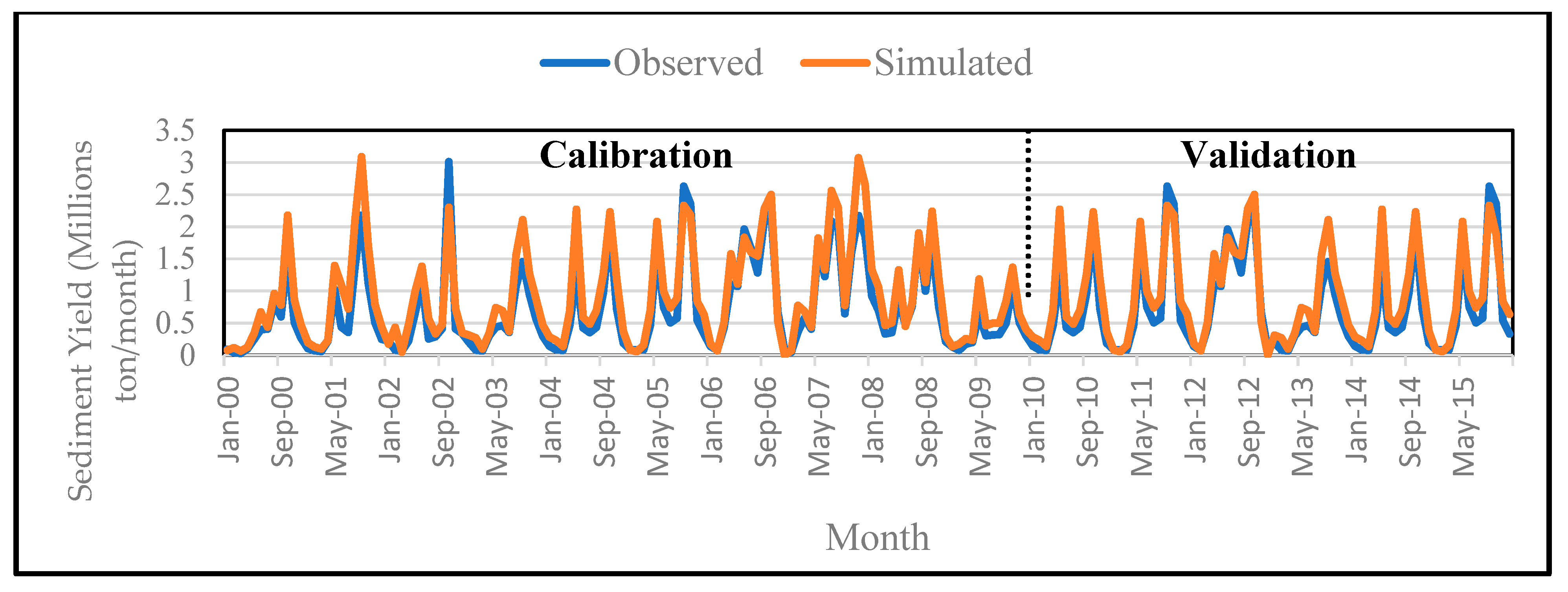
2.7. Model Calibration and Validation

For the purposes of calibration and validation of the SWAT model, the daily discharge data of the river were obtained from the MoWE of Ethiopia, while the sediment data were generated using the sediment discharge rating curve from the Rift Valley Lake Basin Master Plan study [44] with an R2 value of 0.8. For calibration and validation of the model, the bed load component of the sediment was considered suspended as the model simulates total sediment load plus bed load, which was commonly overlooked in most studies in the country due to measurement limitations. In most streams, bed load to suspended load varies from 10% to 30% [56]. For instance, a study in the Ziway Lake Basin in Ethiopia [3] used 10% of the suspended sediment as bed load. Since Lake Ziway and Gidabo River are located in the Ethiopian Rift Valley, we assumed the bed load as 10% of the suspended sediment load gained from the rating curve, which was included for model calibration.
The SWAT model was calibrated and validated to ensure its ability to prioritize the sub-watershed according to sediment contribution. The model was run for the simulation period of 1 January 1998 through December 2015 for the Measso gauging station. River discharge and sediment data over 10 years from 2001 to 2010 were used for calibration, and data from the subsequent 5 years (2011–2015) were then used for the validation period. The first 3 years in the calibration run were used for model preparation. For this study, the duration lengths used for calibration and validation were fixed according to the observed data records. The sensitivity analyses were conducted automatically using the SUFI-2 program in SWATCUP software during calibration.

2.8. Quality Control and Statistical Analysis of Data

Checking for continuity and consistency of both metrological and hydrological data is required before using them for further analysis. Quality assessment and filling of data gaps are needed for the analyses. Continuous daily series data are exposed to outliers caused by instrumental and/or human error. To perceive these outliers, concentrations less than half or more than twice the expected amount were removed from further analysis according to Grubb’s test method [57]. No more than 1% of the dataset was rejected in all cases. Four broadly used statistical indices, namely, the Nash–Sutcliffe coefficient (NSE), percentage bias (PBIAS), coefficient of determination (R2), and RSR (ratio of the root-mean-square error (RMSE)) were used to evaluate model performance by fitting the measured constituent data to the standard deviation of the measured data [58].

3. Results and Discussion

3.1. Stream Flow Simulation

3.1.1. Analysis of Sensitivity

To find the most sensitive model parameter in the Gidabo watershed, a stream flow sensitivity analysis was carried out after simulating the model using daily data. A total of 10 parameters were used for sensitivity analysis, and the parameters governing runoff in the Gidabo watershed were ranked as high, medium, and low according to the associated p-value and equivalent t-stat value; the results are shown in Table 2.

3.1.2. Stream Flow Calibration and Validation

The six most influential flow parameters with high and medium sensitivity (Table 2) were used for further iterations in the calibration period (Table 3).
The model performance evaluation result is presented in Table 4 according to [58]. The result of flow calibration was very good. In a similar manner, for the validation period, the model performance statistics were determined, revealing good results (Table 4). Moreover, the graphical representations of measured and simulated stream flows correlated well for both calibration and validation periods (Figure 5).

3.1.3. Water Balance Components

The Gidabo watershed annual water balance components were simulated by the SWAT model using the principle of conservation of mass. The simulated annual water balance components showed that an average annual precipitation of 1400.4 mm and evaporation loss of 652.7 mm in the basin, accounting for 49.95% of the annual water budget. Surface runoff (SURQ), lateral flow (LATQ), and ground water flow (GWQ) were 342.24 mm (19.58%), 275.6 mm (8.17%), and 21.35 mm (6.82%), respectively. The average stream flow (WYLD) is a combination of surface runoff, lateral, and ground water flow, and it accounted for 421.63 mm (34.57%) of the annual water budget. The deep percolation (PERCOLATE) and initial soil water content (SWo) accounted for 107.10 mm (8.78%) and 167.14 mm (13.71%), respectively, of the annual water budget. The final soil water content (SWt) determined using the water balance equation was 81.72 mm.
The water yield of ungauged regions was estimated using an empirical regression model relating the flow of gauged stations (Aposto, Kolla, Badessa and Measso) to several catchment characteristics, namely, drainage area, slope, and average annual rainfall. As a result, the average annual flow rate of ungauged regions was determined as 2201.714 CMC.

3.2. Sediment Yield Simulation

3.2.1. Sensitivity Analysis

Twelve sediment parameters were checked using SUFI-2 in SWAT-CUP to identify the most sensitive parameters (Table 5).

3.2.2. Sediment Yield Calibration and Validation

After stream flow calibration, sediment flow calibration was conducted using sensitive parameters related to soil loss from each HRU. To determine the magnitude of catchment sediment yield, the initial sensitive sediment parameters were calibrated using the global sensitivity analysis procedure. As a result, nine parameters with high to medium sensitivity (Table 6) were identified for sediment calibration process.
As shown in Figure 6, the calibration of the SWAT model was successfully achieved using the observed daily sediment flow. Similarly, during the validation stage, the SWAT model adequately mimicked the sediment inflow of the river.
According to the outcome of calibration and validation, the model performance was examined according to statistical indicators (Table 7).
As can be seen in Table 7, all numerical model performance measures were in an acceptable range, indicating that the SWAT model replicated the observed sediment yields. Similarly, the graphical representation of measured and simulated flows correlated well for both calibration and validation periods (Figure 6). Hence, the result can be used to identify major sediment source areas within the sub-watersheds.

3.3. Spatial Distribution of Sediment Generation Hotspot Areas

The calibrated and validated SWAT model was used to simulate the effect of management/conservation measures on water and sediment yield in the watershed. The spatial variability of erosion rate was identified as shown in Figure 7.
The spatial variability of sediment yield for the Gidabo watershed was identified from the simulated annual sediment yield, and the result ranged from 1.44 to 23.85 tons/ha/year with an average of 11.46 tons/ha/year for the sub-basins. Sub-basins 2, 21, and 22 yielded very high sediment (20 to 25 tons/ha/year), sub-basins 1, 3, 5, 19, 20, and 23 yielded high sediment (15 to 20 tons/ha/year), sub-basins 4, 6, 8, and 12 yielded moderate sediment (10 to 15 tons/ha/year), sub-basins 7, 9, 10, 11, 13, and 14 yielded low sediment (5 to 10 tons/ha/year), and sub-basins 15, 16, 17, and 18 yielded very low sediment (0 to 5 tons/ha/year). The average annual sediment yield from the total watershed was estimated as 2.92 million tons/year.
To quantify the effects of catchment characteristics on the sediment yield rates of the sub-basin, the correlation of hotspot areas and catchment characteristics was determined.
As indicated in Table 8, all of the selected catchments in areas with high erosion risk (sub-basins 22, 2, 1, 19, and 3) were characterized by a single land-use class (agricultural) and one soil type (Chromic). Furthermore, the catchment prioritization study showed that soil loss is modest in low-lying locations with the same land use and soil type. This indicates that the variation of sediment yield is more sensitive to terrain slopes due to poor land-use practices in steep areas.
On the basis of this finding, potential areas of intervention were prioritized, and four management scenarios were designed and simulated using the SWAT model in order to assess the basin’s most appropriate management/conservation actions: scenario I (grassed waterway), scenario II (filter strip), scenario III (terracing), and scenario IV (contouring). The baseline scenario was used as a reference for comparisons of the effectiveness of the developed sediment reduction scenarios (Table 9).
In conclusion, after the application of terracing, the greatest reduction in sediment yield (62.32%) was observed. As the Gidabo irrigation dam is located at the outlet of the Measso gauging station (where the river basin was modeled), the application of the best selected scenario would decrease the sedimentation rate of the dam by 62.32%.

4. Conclusions

The goal of this research was to use the SWAT model to analyze surface runoff generation and soil erosion rates in the Gidabo watershed. Both runoff and sediment fluxes were calibrated and validated using field-measured soil characteristics. To assess the degree of connection between measured and simulated monthly datasets, the sensitive flow and sediment parameters were considered in the process of calibration. During both calibration and validation periods, the model’s performance was determined to be very good for both stream and sediment flow.
For each HRU, the sediment yield validated using the Soil and Water Assessment Tool model was shown to be correlated with land use, soil, and topography. Possible sediment basin regions for watershed prioritization and erosion regulation were distinguished on the basis of the sediment yield of the sub-basins. All of the sub-basins identified as sedimentation source locations shared a typical soil type and a typical land-use class, with varying terrain slopes. This shows that the difference in sediment yield is more sensitive to terrain slopes because of poor catchment management in steep areas. Moreover, the study findings indicated that the best choice to lessen the sediment flow of the watershed is to apply soil protection practices that decrease the catchment slope length. Accordingly, the application of terracing would result in the greatest reduction in sediment yield (62.32%).
In order to decrease the land degradation of the watershed and lengthen the beneficial lifespan of the dam located below the watershed, an organized strategy might be required. As a result, the produced map (Figure 7) indicating high-erosion areas can be used by decision-makers to undertake appropriate soil conservation measures in particular areas. In these erosion-prone areas, mandatory actions may also include strip planting, terracing, or contour farming to decrease the effect of the slope on surface runoff flow velocity and sediment transport capacity.

Author Contributions

Conceptualization, M.D. and A.O.A.; methodology; software; validation, P.Y. and L.S.; formal analysis, A.O.A.; investigation, P.Y.; resources, L.S.; data curation, M.D.; writing—original draft preparation, A.O.A.; writing—review and editing, M.D.; visualization, P.Y. and L.S.; supervision, L.S.; project administration, M.D.; funding acquisition, P.Y. All authors have read and agreed to the published version of the manuscript.

Funding

This research was funded by Hawassa University Institute of Technology Thematic Research Project Grant.

Data Availability Statement

Data can be provided upon request.

Acknowledgments

This study was financed by the Hawassa University Institute of Technology Thematic Research Projects Fund. The authors would like to thank the Ethiopian National Meteorological Service Agency and Ministry of Water and Energy for providing the necessary data.

Conflicts of Interest

The authors declare no conflict of interest.

References

  1. Aga, A.O.; Melesse, A.M.; Chane, B. Estimating the Sediment Flux and Budget for a Data Limited Rift Valley Lake in Ethiopia. Hydrology 2018, 6, 1. [Google Scholar] [CrossRef] [Green Version]
  2. Cuceloglu, G.; Abbaspour, K.C.; Ozturk, I. Assessing the Water-Resources Potential of Istanbul by Using a Soil and Water Assessment Tool (SWAT) Hydrological Model. Water 2017, 9, 814. [Google Scholar] [CrossRef] [Green Version]
  3. Aga, A.O.; Chane, B.; Melesse, A.M. Soil Erosion Modelling and Risk Assessment in Data Scarce Rift Valley Lake Regions, Ethiopia. Water 2018, 10, 1684. [Google Scholar] [CrossRef] [Green Version]
  4. Aga, A.O.; Melesse, A.M.; Chane, B. An Alternative Empirical Model to Estimate Watershed Sediment Yield Based on Hydrology and Geomorphology of the Basin in Data-Scarce Rift Valley Lake Regions, Ethiopia. Geosciences 2020, 10, 31. [Google Scholar] [CrossRef] [Green Version]
  5. Defersha, M.B.; Melesse, A.M. Field-scale investigation of the effect of land use on sediment yield and runoff using runoff plot data and models in the Mara River basin, Kenya. Catena 2012, 89, 54–64. [Google Scholar] [CrossRef]
  6. Defersha, M.B.; Melesse, A. Effect of rainfall intensity, slope and antecedent moisture content on sediment concentration and sediment enrichment ratio. Catena 2012, 90, 47–52. [Google Scholar] [CrossRef]
  7. Melesse, A.; Abtew, W. Landscape Dynamics, Soils and Hydrological Processes in Varied Climates; Springer: Berlin/Heidelberg, Germany, 2015; ISBN 978-3-319-18787-7. [Google Scholar]
  8. Yesuf, H.M.; Assen, M.; Alamirew, T.; Melesse, A. Modeling of sediment yield in Maybar gauged watershed using SWAT, northeast Ethiopia. Catena 2015, 127, 191–205. [Google Scholar] [CrossRef]
  9. Cheng, P.-D.; Zhu, H.-W.; Fan, J.-Y.; Fei, M.-R.; Wang, D.-Z. Numerical research for contaminant release from un-suspended bottom sediment under different hydrodynamic conditions. J. Hydrodyn. 2013, 25, 620–627. [Google Scholar] [CrossRef]
  10. Wang, F.; Mu, X.; Li, R.; Fleskens, L.; Stringer, L.C.; Ritsema, C.J. Co-evolution of soil and water conservation policy and human–environment linkages in the Yellow River Basin since 1949. Sci. Total Environ. 2015, 508, 166–177. [Google Scholar] [CrossRef] [Green Version]
  11. Terskii, P.; Kuleshov, A.; Chalov, S.; Terskaia, A.; Belyakova, P.; Karthe, D.; Pluntke, T. Assessment of Water Balance for Russian Subcatchment of Western Dvina River Using SWAT Model. Front. Earth Sci. 2019, 7, 241. [Google Scholar] [CrossRef]
  12. Valjarević, A.; Djekić, T.; Stevanović, V.; Ivanović, R.; Jandziković, B. GIS numerical and remote sensing analyses of forest changes in the Toplica region for the period of 1953–2013. Appl. Geogr. 2018, 92, 131–139. [Google Scholar] [CrossRef]
  13. Micić, P.; Lukić, T.; Basarin, T.; Jokić, B.; Wilby, M.; Pavić, R.L.; Mesaroš, D.; Valjarević, M.; Milanovic, A.; Morar, M.M. Detailed Analysis of Spatial-Temporal Variability of Rainfall Erosivity and Erosivity Density in the Central and Southern Pannonian Basin. Sustainability 2021, 13, 13355. [Google Scholar] [CrossRef]
  14. Aliye, M.A.; Aga, A.O.; Tadesse, T.; Yohannes, P. Evaluating the Performance of HEC-HMS and SWAT Hydrological Models in Simulating the Rainfall-Runoff Process for Data Scarce Region of Ethiopian Rift Valley Lake Basin. Open J. Mod. Hydrol. 2020, 10, 105–122. [Google Scholar] [CrossRef]
  15. Yu, B.; Neil, D. Temporal and Spatial Variation of Sediment Yield in the Snowy Mountains Region, Australia. In Variability in Stream Erosion and Sediment Transport, Proceedings of the Canberra Symposium, Canberra, Australia, 5–9 December 1994; IAHS Publications: Wallingford, UK, 1994; Volume 224. [Google Scholar]
  16. Marttila, H.; Bjørn, K. Dynamics of Erosion and Suspended Sediment Transport from Drained Peatland Forestry. J. Hydrol. 2010, 388, 414–425. [Google Scholar] [CrossRef]
  17. Arekhi, S.; Niazi, Y.; Kalteh, A.M. Soil erosion and sediment yield modeling using RS and GIS techniques: A case study, Iran. Arab. J. Geosci. 2012, 5, 285–296. [Google Scholar] [CrossRef]
  18. Salsabilla, A.; Kusratmoko, E. Assessment of soil erosion risk in Komering watershed, South Sumatera, using SWAT model. AIP Conf. Proc. 2017, 1862, 30192. [Google Scholar] [CrossRef] [Green Version]
  19. Bisantino, T.; Bingner, R.; Chouaib, W.; Gentile, F.; Liuzzi, G.T. Estimation of Runoff, Peak Discharge and Sediment Load at the Event Scale in a Medium-Size Mediterranean Watershed Using the Annagnps Model: An AGNPS Evaluation for Runoff, Peak Discharge and Sediment Load. Land Degrad. Dev. 2015, 26, 340–355. [Google Scholar] [CrossRef]
  20. Chu, T.W.; Shirmohammadi, A.; Montas, H.; Sadeghi, A. Evaluation of the swat model’s sediment and nutrient components in the piedmont physiographic region of maryland. Trans. ASAE 2004, 47, 1523–1538. [Google Scholar] [CrossRef]
  21. Muleta, M.K.; Nicklow, J.W. Decision Support for Watershed Management Using Evolutionary Algorithms. J. Water Resour. Plan. Manag. 2005, 131, 35–44. [Google Scholar] [CrossRef]
  22. Jha, M.K.; Gassman, P.W.; Arnold, J.G. Water Quality Modeling for the Raccoon River Watershed Using SWAT. Trans. ASABE 2007, 50, 479–493. [Google Scholar] [CrossRef]
  23. Akoko, G.; Le, T.; Gomi, T.; Kato, T. A Review of SWAT Model Application in Africa. Water 2021, 13, 1313. [Google Scholar] [CrossRef]
  24. Dessu, S.B.; Melesse, A.M.; Bhat, M.G.; McClain, M.E. Assessment of water resources availability and demand in the Mara River Basin. Catena 2014, 115, 104–114. [Google Scholar] [CrossRef]
  25. Dessu, S.; Melesse, A.M. Modelling the Rainfall–Runoff Process Ofthe Mara River Basin Using the Soil and Water Assessment Tool. Hydrol. Process. 2012, 26, 4038–4049. [Google Scholar] [CrossRef]
  26. Dessu, S.B.; Melesse, A.M. Impact and uncertainties of climate change on the hydrology of the Mara River basin, Kenya/Tanzania. Hydrol. Process. 2012, 27, 2973–2986. [Google Scholar] [CrossRef]
  27. Setegn, S.G.; Srinivasan, R.; Dargahi, B.; Melesse, A.M. Spatial delineation of soil erosion vulnerability in the Lake Tana Basin, Ethiopia. Hydrol. Process. 2009, 23, 3738–3750. [Google Scholar] [CrossRef]
  28. Setegn, S.G.; Dargahi, B.; Srinivasan, R.; Melesse, A. Modeling of Sediment Yield From Anjeni-Gauged Watershed, Ethiopia Using SWAT Model1. JAWRA J. Am. Water Resour. Assoc. 2010, 46, 514–526. [Google Scholar] [CrossRef]
  29. Setegn, S.G.; Srinivasan, R.; Melesse, A.M.; Dargahi, B. SWAT model application and prediction uncertainty analysis in the Lake Tana Basin, Ethiopia. Hydrol. Process. 2009, 24, 357–367. [Google Scholar] [CrossRef]
  30. Setegn, S.G.; Rayner, D.; Melesse, A.; Dargahi, B.; Srinivasan, R. Impact of climate change on the hydroclimatology of Lake Tana Basin, Ethiopia. Water Resour. Res. 2011, 47, W04511. [Google Scholar] [CrossRef]
  31. Aga, A.O. Modeling Sediment Yield, Transport and Deposition in the Data Scarce Region of Ethiopian Rift Valley Lake Basin. Ph.D. Dissertation, Addis Ababa University, Addis Ababa, Ethiopia, 2019. [Google Scholar]
  32. Nguyen, V.T.; Dietrich, J.; Uniyal, B.; Tran, D.A. Verification and Correction of the Hydrologic Routing in the Soil and Water Assessment Tool. Water 2018, 10, 1419. [Google Scholar] [CrossRef] [Green Version]
  33. Parajuli, P.B.; Nelson, N.O.; Frees, L.D.; Mankin, K.R. Comparison of AnnAGNPS and SWAT model simulation results in USDA-CEAP agricultural watersheds in south-central Kansas. Hydrol. Process. 2009, 23, 748–763. [Google Scholar] [CrossRef]
  34. Chang, C.; Harrison, J.F.; Huang, Y. Modeling Typhoon-Induced Alterations on River Sediment Transport and Turbidity Based on Dynamic Landslide Inventories: Gaoping River Basin, Taiwan. Water 2015, 7, 6910–6930. [Google Scholar] [CrossRef] [Green Version]
  35. Guo, S.; Zhu, Z.; Lyu, L. Effects of Climate Change and Human Activities on Soil Erosion in the Xihe River Basin, China. Water 2018, 10, 1085. [Google Scholar] [CrossRef] [Green Version]
  36. Li, D.; Qu, S.; Shi, P.; Chen, X.; Xue, F.; Gou, J.; Zhang, W. Development and Integration of Sub-Daily Flood Modelling Capability within the SWAT Model and a Comparison with XAJ Model. Water 2018, 10, 1263. [Google Scholar] [CrossRef] [Green Version]
  37. Mishra, Y.; Nakamura, T.; Babel, M.S.; Ninsawat, S.; Ochi, S. Impact of Climate Change on Water Resources of the Bheri River Basin, Nepal. Water 2018, 10, 220. [Google Scholar] [CrossRef] [Green Version]
  38. Qi, Z.; Kang, G.; Chu, C.; Qiu, Y.; Xu, Z.; Wang, Y. Comparison of SWAT and GWLF Model Simulation Performance in Humid South and Semi-Arid North of China. Water 2017, 9, 567. [Google Scholar] [CrossRef] [Green Version]
  39. Grey, O.P.; Webber, D.F.S.G.; Setegn, S.G.; Melesse, A.M. Application of the Soil and Water Assessment Tool (SWAT Model) on a Small Tropical Island (Great River Watershed, Jamaica) as a Tool in Integrated Watershed and Coastal Zone Management. Rev. Biol. Trop. 2014, 62, 293–305. [Google Scholar] [CrossRef] [Green Version]
  40. Haregeweyn, N.; Berhe, A.; Tsunekawa, A.; Tsubo, M.; Meshesha, D.T. Integrated Watershed Management as an Effective Approach to Curb Land Degradation: A Case Study of the Enabered Watershed in Northern Ethiopia. Environ. Manag. 2012, 50, 1219–1233. [Google Scholar] [CrossRef]
  41. Gashaw, T.; Tulu, T.; Argaw, M. Erosion risk assessment for prioritization of conservation measures in Geleda watershed, Blue Nile basin, Ethiopia. Environ. Syst. Res. 2017, 6, 1. [Google Scholar] [CrossRef]
  42. Osore, A.; Moges, A. Extent of Gully Erosion and Farmer’s Perception of Soil Erosion in Alalicha Watershed, Southern Ethiopia. J. Environ. Earth Sci. 2014, 4, 74–81. [Google Scholar]
  43. Tongul, H.; Hobson, M. Scaling up an Integrated Watershed Management Approach through Social Protection Programmes in Ethiopia: The MERET and PSNP Schemes. In Proceedings of the Hunger, Nutrition and Climate Justice Conference 2013, Dublin, Ireland, 15–16 April 2013. [Google Scholar]
  44. MOWR The Federal Democratic Republic of Ethiopia-Ministry of Water Resources. Rift Valley Lakes Basin Integrated Resources Development Master Plan Study Project. Halcrow Group Limited and Generation Integrated Rural Development (GIRD) Consultants. Addis Ababa, Ethiopia. 2010; unpublished. [Google Scholar]
  45. Shi, P.; Ma, X.; Hou, Y.; Li, Q.; Zhang, Z.; Qu, S.; Chen, C.; Cai, T.; Fang, X. Effects of Land-Use and Climate Change on Hydrological Processes in the Upstream of Huai River, China. Water Resour. Manag. 2012, 27, 1263–1278. [Google Scholar] [CrossRef]
  46. Xie, X.; Cui, Y. Development and test of SWAT for modeling hydrological processes in irrigation districts with paddy rice. J. Hydrol. 2011, 396, 61–71. [Google Scholar] [CrossRef]
  47. Mckeever, V. National Engineering Handbook; Section 4: Hydrology; US Soil Conservation Service: Washington, DC, USA, 1972. [Google Scholar]
  48. Monteith, J. Evaporation and Environment. Symposia of the Society for Experimental Biology. Symp. Soc. Exp. Biol. 1965, 19, 205–234. [Google Scholar] [PubMed]
  49. Kumar, M.; Kumar, N.R.; Reddy, K.; Rao, C.S. Spatial Modeling of Evapotranspiration for Efficient Water Management at Regional Scale. Indian J. Dryland Agric. Res. Dev. 2014, 29, 23–27. [Google Scholar] [CrossRef]
  50. Hargreaves, B.G.H. Reference evapotranspiration By George H. Hargreaves, 1 Fellow, ASCE. J. Irrig. Drain. Eng. 1994, 120, 1132–1139. [Google Scholar] [CrossRef]
  51. Arekhi, S.; Shabani, A.; Rostamizad, G. Application of the modified universal soil loss equation (MUSLE) in prediction of sediment yield (Case study: Kengir Watershed, Iran). Arab. J. Geosci. 2011, 5, 1259–1267. [Google Scholar] [CrossRef]
  52. Neitsch, S.L.; Arnold, J.G.; Kiniry, J.R.; Williams, J.R. Soil & Water Assessment Tool Theoretical Documentation Version 2009; Texas Water Resources Institute: College Station, TX, USA, 2011; pp. 1–647. [Google Scholar]
  53. Shao, G.; Wu, J. On the accuracy of landscape pattern analysis using remote sensing data. Landsc. Ecol. 2008, 23, 505–511. [Google Scholar] [CrossRef]
  54. Sharply, A.N.; Williams, J.R. EPIC-Erosion/Productivity Impact Calculator I, Model Documentation. USDA Tech. Bull. 1990, 1759, 235. [Google Scholar]
  55. Liersch, S. The Program PcpSTAT User’s Manua, 2003. Available online: www.swat.tamu.edu/sofware/swat-model (accessed on 9 April 2022).
  56. Church, M. Bed material transport and the morphology of alluvial river channels. Annu. Rev. Earth Planet. Sci. 2006, 34, 325–354. [Google Scholar] [CrossRef]
  57. Grubbs, F.F. Procedures for Detecting Outlying Observations in Samples. Technometrics 1969, 11, 1–21. [Google Scholar] [CrossRef]
  58. Moriasi, D.N.; Arnold, J.G.; van Liew, M.W.; Bingner, R.L.; Harmel, R.D.; Veith, T.L. Model evaluation guidelines for systematic quantification of accuracy in watershed simulations. Trans. ASABE 2007, 50, 885–900. [Google Scholar] [CrossRef]
Figure 1. Study area map.
Sustainability 14 05262 g001
Figure 2. Average annual rainfall depth (1998–2017) in Gidabo watershed (source: National Meteorological Agency of Ethiopia).
Sustainability 14 05262 g002
Figure 3. (a) Gidabo LULC map; (b) Gidabo soil map.
Sustainability 14 05262 g003
Figure 4. Gidabo river basin monitoring gauge stations collected from the MoWE.
Sustainability 14 05262 g004
Figure 5. Monthly observed and simulated flow hydrograph during calibration and validation periods at Measso gauging station.
Sustainability 14 05262 g005
Figure 6. Monthly observed and simulated sediment yield graph during calibration and validation periods at Measso gauging station.
Sustainability 14 05262 g006
Figure 7. Spatial distribution of soil loss severity classes.
Sustainability 14 05262 g007
Table 1. Meteorological stations in and around the study area.
NoStationLatLongRain FallMin TempMax TempSolar RadiationRelative HumidityWind Speed
1Kebado426,275.41711,154.28XXX
2Dilla422,582.85703,793.12
3Yigalem432,892.4753,542.37XXX
4Yirga chefe411,707.53679,925.57XXX
5Aleta Wendo435,670.37729,998.10XXX
Table 2. Ranking of sensitive flow parameters identified in the Gidabo watershed.
Parameters Descriptiont-Statp-ValueSensitivityRank
Alpha base flow recession constant (ALPHA_BF)−8.3590 High1
Effective hydraulic conductivity of main channel (CH_K2)−2.6980.007High2
Threshold depth of water in the shallow aquifer for return flow to occur (GWQMN)1.9290.054High3
Groundwater delay (GW_DELAY)1.1580.247High4
Biological mixing efficiency (BIOMIX)0.8720.383Medium5
SCS runoff curve number (CN2)0.6640.507Medium6
Groundwater “revap” coefficient (GW_REVAP)−0.3470.729Medium7
Soil evaporation compensation factor (ESCO)−0.2950.768Medium8
Maximum canopy storage (CANMX)−0.0710.944Medium9
Threshold depth of water in the (GWQMN)−0.0170.986Medium10
Table 3. Summary of calibrated flow parameters.
Parameters DescriptionRange ValueFitted ValuesRank
Alpha base flow recession constant (ALPHA_BF)0–10.051
Effective hydraulic conductive of maim channel (CH_K2)0–150136.272
Threshold depth of water in the shallow aquifer for return flow to occur (GWQMN)0–50001.88493
Groundwater delay (GW_DELAY)0–50029.754
Biological mixing efficiency (BIOMIX)0–10.325
SCS runoff curve number (CN2)35–980.266
Table 4. Calibrated and validated model performance indicators.
Gauging StationSimulation PeriodUncertainty MeasuresModel Performance Indicators
P-FactorR-FactorR2ENSRSRPBIAS
MeassoCalibration0.780.490.850.780.46−9.4
Validation0.760.520.830.770.51−8.3
Table 5. Ranking of sensitive sediment parameters identified in the Gidabo watershed.
ParametersDescriptiont-statp-ValueSensitivityRank
CN2SCS runoff curve number−18.6830High1
CANMXMaximum canopy storage8.4240High2
ALPHA_BFAlpha base flow recession constant1.5710.117High3
USLE_PUSLE support practice factor0.9270.355High4
GWQMNThreshold depth of water in the shallow aquifer for return flow to occur0.8630.389High5
GW_DELAYGroundwater delay0.5540.58Medium6
SPEXPExponential factor for channel sediment routing−0.5170.606Medium7
CH_COV1Channel erodibility factor0.5030.615Medium8
USLE_KSaturated hydraulic conductivity0.3020.763Medium9
SPCONLinear factor for the channel sediment routing0.2020.839Low10
TIMPSnow pack temperature lag factor0.2000.952Low11
GW_REVAPGroundwater revamp coefficient0.0291.007Low12
Table 6. Nine sediment calibration parameters selected in the Gidabo watershed.
ParametersDescriptionRange ValueFitted ValueRank
CN2SCS runoff curve number35–980.231
CANMXMaximum canopy storage0–106.72
ALPHA_BFAlpha base flow recession constant0–10.873
USLE_PUSLE support practice factor0–10.884
GWQMNThreshold depth of water in the shallow aquifer for return flow to occur0–50003298.575
GW_DELAYGroundwater delay0–500291.726
SPEXPExponential factor for channel sediment routing1–21.777
CH_COV1Channel erodibility factor0–10.418
SOL_KSaturated hydraulic conductivity0-200060.639
Table 7. Model performance statistics measured and simulated sediment yield calibration and validation.
Gauging StationSimulation PeriodUncertainty MeasuresModel Performance Indicators
P-FactorR-FactorR2ENSRSRPBIAS
MeassoCalibration0.730.430.810.760.43−8.8
Validation0.80.440.840.780.46−10.2
Table 8. Thirteen erosion-affected sub-basins and their SWAT-simulated land use/cover, soil, and slope.
Sub BasinArea (km2)SWAT Dominant Land Use/CoverSWAT Dominant Soil TypeMean Slope (%)Sediment Yield (tons/ha/year)
2295.44AGRL and RNGBDystric, Eutric, Chromic, and Orthic19.5523.85
2160.63AGRLChromic and Orthic18.6720.79
2113.42AGRL and RNGBChromic and Eutric17.8020.53
1236.72AGRLOrthic, Chromic, and Pellic16.8018
1987.53AGRL and RNGBChromic, Calcic, Eutric, and Dystric15.2517.2
3159.83AGRL and AGRCPellic, Chromic, Orthic, and Eutric13.7616.56
2092.60AGRL, AGRC,
RNGB, and FRST
Eutric, Chromic, and Eutric11.8416.48
587.60AGRL and AGRCPellic and Eutric18.5716.05
23235.59AGRLEutric, Chromic, and Eutric17.2615.15
663.84AGRL, AGRC, and FRSTPellic and Eutric15.9613.15
12116.94RNGB and AGRLEutric, Calcic, Chromic, and Pellic11.8712.82
484.03AGRL, FRST, and AGRCEutric, Chromic, Pellic, and Orthic14.2712.79
8220.23AGRL and AGRCChromic, Eutric, Chromic, Pellic, and Orthic12.8411.65
Table 9. Estimated sediment reduction due to conservation structures and best management practices as compared to the baseline scenario.
ScenariosMean Annual Sediment Yield Reduction
Sediment Reduction (tons/ha/year)Sediment Percentage of Reduction
Baseline condition11.46100
Grassed waterway5.8449
Filter strips7.1637.53
Terracing4.3262.32
Contouring5.254.6
The reductions in sediment yield for grassed waterway, filter strip, terracing, and contouring were 49%, 37.53%, 62.32%, and 54.6%, respectively.
Publisher’s Note: MDPI stays neutral with regard to jurisdictional claims in published maps and institutional affiliations.

