Article

Understanding the Correlation of Demographic Features with BEV Uptake at the Local Level in the United States

Durham School of Architectural Engineering and Construction, University of Nebraska-Lincoln, Omaha, NE 68182, USA
*
Author to whom correspondence should be addressed.
Sustainability 2022, 14(9), 5016; https://doi.org/10.3390/su14095016
Submission received: 4 February 2022 / Revised: 20 April 2022 / Accepted: 20 April 2022 / Published: 22 April 2022

Abstract

:
Battery Electric Vehicles (BEVs) have seen a substantial growth in the recent past, and this trend is expected to continue. This growth has been far from uniform geographically, with large differences in BEV uptake between countries, states, and cities. This non-uniform growth can be attributed to the demographic and non-demographic factors that characterize a geographical location. In this paper, the demographic factors that affect BEV uptake at the Zone Improvement Plan (ZIP) code level are studied extensively across several states in the United States to understand BEV readiness at its most granular form. Demographic statistics at the ZIP code level more accurately describe the local population than national-, state-, or city-level demographics. This study compiled and preprocessed 242 demographic features to study the impact on BEV uptake in 7155 ZIP codes in 11 states. These demographic features are categorized based on the type of information they convey. The initial demographic features are subjected to feature engineering using various formed hypotheses to extract the optimal level of information. The hypotheses are tested and a total of 82 statistically significant features are selected. This study used correlation analysis to validate the feature engineering and understand the degree of correlation of these features to BEV uptake, both within individual states and at the national level. Results from this study indicate that higher BEV adoption in a state results in a stronger correlation between demographic factors and BEV uptake. Features related to the number of individuals in a ZIP code with an annual income greater than USD 75 thousand are strongly correlated with BEV uptake, followed by the number of owner-occupied housing units, individuals driving alone, and working from home. Features containing compounded information from distinct categories are often better correlated than features containing information from a single category. In-depth knowledge of local BEV uptake is important for applications related to the accommodation of BEVs, and understanding what causes differences in local uptake can allow for both the prediction of future growth and the stimulation of it.

1. Introduction

Battery Electric Vehicles (BEVs) have gained popularity in the last few years, with the advancement of battery technology, increase in charging infrastructures, and rising concerns over greenhouse emissions from conventional vehicles. Although there has been a considerable growth in BEV uptake, the slope of this growth is not consistent across countries, or even within individual US states. There are several factors that affect BEV uptake, including the availability of charging infrastructures, public incentives, socio-demographic factors, psychological factors, and environmental awareness.
Charging infrastructure planning requires the proper understanding of the BEV uptake at the local level for the optimal selection of the sites. Incentives have been partially effective in the promotion of the BEV technology. Many states have incentives in place to help offset the high initial cost of BEVs. The federal government tax credit is up to USD 7500 [1] for BEVs with a minimum onboard battery capacity of 4 kWh. Understanding the socio-demographic factors is important to help accelerate the BEV uptake at the local level. Previous researchers have used survey data to characterize the early adopters of BEVs and understand the intention of purchasing BEVs. It is important to empirically study the numerous socio-demographic factors that impact actual local BEV uptake, particularly in the US.
The availability of charging infrastructures is cited as one of the most key factors in the available literature. Planning the optimal installation of charging infrastructures requires an understanding of BEV uptake and user behavior. In reference [2], the authors discussed direct and indirect factors that influence the development of charging infrastructures to aid the development of the EV market. The charging demand of the location, the economics of installing and maintaining a charging station, and financial incentives have direct impacts on their deployment. Indirect factors cited in reference [2] include the psychological behavior of EV users, policy changes towards EV use, and the development of battery technologies. In reference [3], the planning and installation of charging infrastructures and EV uptake is what is referred to as a chicken-and-egg problem, where EV uptake is said to impact and be affected by these installations. The authors propose a framework where the number of EVs are reinforced in a feedback loop for the planning of the charging infrastructures. The economic factors discussed in the paper are only considered for better understanding the EV uptake.
Identifying the optimal locations for charging infrastructures has been challenging without prior knowledge of BEV uptake in each area. In references [4,5,6,7], the authors have developed an algorithm that determines the number of charging infrastructures required in highway corridors for the state of Nebraska for different-range EVs, considering full bidirectional coverage. However, with limitations to proper funding to planning agencies, not all the corridors have been provided with charging infrastructures [8]. Additionally, priority locations identified in these papers do not include the impact of the demographic factors. In most cases, charging infrastructures are planned based on travel demand [9], urban setup [10,11], and charging demand prediction [12,13]. The literature relies on calculations based on survey data. Accurately generalizing such data to the greater population of an area requires an extensive understanding of the demographics of each region.
Socio-demographic factors play an important role in understanding both actual BEV adoption and BEV purchase intention. Several studies in European countries have summarized the socio-demographic factors at the national level using surveys to study BEV purchase intention. In reference [14], the authors have presented socio-demographic factors as control variables to EV purchase intention. The socio-demographic factors that are discussed are age, level of education, gender, vehicles owned, household size, and travel patterns. In reference [15], a survey is conducted in Austria where socio-demographic factors are studied along with psychological factors to understand whether an individual is willing to adopt an EV. In reference [16], socio-demographic factors are studied using hierarchical regression to understand EV adoption interest from online surveys across the Scandinavian countries. Similar studies are conducted in references [17,18,19] regarding BEV purchase intention in China, a leader in the BEV market. Charging infrastructure availability, environmental awareness, and EV price are determined to be important. Among demographic factors, age, gender, income, education, marital status, and household size are analyzed to understand EV purchase intention using correlation.
Survey data can be hard to analyze, as respondents are often exposed to survey fatigue [20], which may lead to biasness in their responses. The questions formulated often are biased in some aspect depending upon the surveyor. In addition, it is necessary to study actual BEV adoption and its relation to demographic factors rather than solely BEV purchase intention, as these numbers can differ in practice. In the US, there are some studies which have used demographic factors at the ZIP code level to understand actual EV adoption. In references [21,22], the authors have studied the socio-demographic factors to understand EV uptake in Hawaii. For this study, 79 ZIP codes are used using negative binomial and ordinary least-squared regression approaches. The dependent variables are log-transformed, and their collinearity is not explained in this study. Education and income are determined to have the most positive impact on EV uptake. In reference [23], the authors developed an ordinary least-squared regression model to study the demographic factors to understand EV and photovoltaic uptake. Additionally studied are 1670 ZIP codes, where median income is determined to have a positive influence on EV uptake, and larger households are determined to influence EV uptake negatively. In reference [24], the authors developed a multiple logistic regression model to assess EV penetration rate with demographic factors. For this study, 58 California counties are used for training the model and nine Delaware Valley counties are used to validate. The authors identified income, education, and the car-sharing status of the household to be the most important in influencing EV adoption.
Understanding the demographic factors at a granular level is important, and the findings can be aggregated to characterize a larger area, such as a city or state. State-level studies [25] provide a coarse presentation about the importance of the factors affecting EV adoption but cannot address the regional variability of the same factors. In reference [26], the authors studied the demographic factors with BEV adoption at an even more granular level than a ZIP code, with 80–120 dwellings in one instance. This level of detail is difficult to replicate at a larger scale due to both limited data resources and privacy and security concerns. In reference [27], the authors studied the capabilities of off-street parking with key demographic information to study which areas have the greater probability to transition to BEVs.
BEV uptake is ultimately affected by a combination of many disparate factors, both demographic and non-demographic. In reference [28], the authors have categorized the non-demographic factors technical, contextual, cost-related, behavioral, and social determinants. They are studied along with socio-demographic factors and BEV-specific experiences to study BEV acceptance. In reference [29], socio-psychological factors are studied to understand the BEV uptake in two cities in China. Socio-psychological factors include technical knowledge about BEVs and policies in effect, neighbor effects, and environmental awareness. In reference [30], a total cost of ownership (TCO) model is developed, where fuel prices are forecasted with the battery pricing of BEVs to study BEV adoption. The price of a BEV is shown to have a greater impact in BEV adoption. Electricity tariffs are also studied in the TCO model, which is dependent on vehicle usage. In references [31,32,33], the authors have developed a charging station network with the simultaneous objectives of reducing range anxiety, minimizing deployment cost, and maintaining the quality of service.
In this paper, a comprehensive study is done to understand the demographic features at the ZIP code level and its correlation with the BEV uptake across 11 states, collectively and individually. While this study isolates quantifiable demographic factors, the comparison of results across states or ZIP codes with disparate non-demographic factors, such as EV policies or fuel prices, can yield information about the net impact of non-demographic factors as well. This study addresses a knowledge gap in quantitative comprehensive studies about demographic factors with BEV uptake at a granular level at a larger scale. BEV uptake has fallen short of expectations and been far from uniform geographically, with large differences in BEV uptake between countries, states, and cities. The geographical differences may be partially explained by the socio-demographic factors that characterize the region. Therefore, there is a need for an extensive study of the socio-demographic factors to understand their effects on BEV uptake within a state and across different states. Performing this analysis at the ZIP code level is particularly important, as characteristics at the state or national level do not accurately reflect the characteristics in a smaller geographical region. The preliminary results of this study have been published in reference [34].
Figure 1 shows the workflow process for the proposed framework in this study. Once collected, the ZIP-code-level data are compiled and preprocessed. The demographic features are grouped based on specific categories and interactions. These groups are then subjected to feature engineering based on formed hypotheses, and thresholds are set. Hypothesis testing is done for all formed hypotheses. Correlation analysis is performed next on the demographic features with the BEV uptake.
The novel contributions of this paper are as follows:
  • Extensive study of 242 socio-demographic factors;
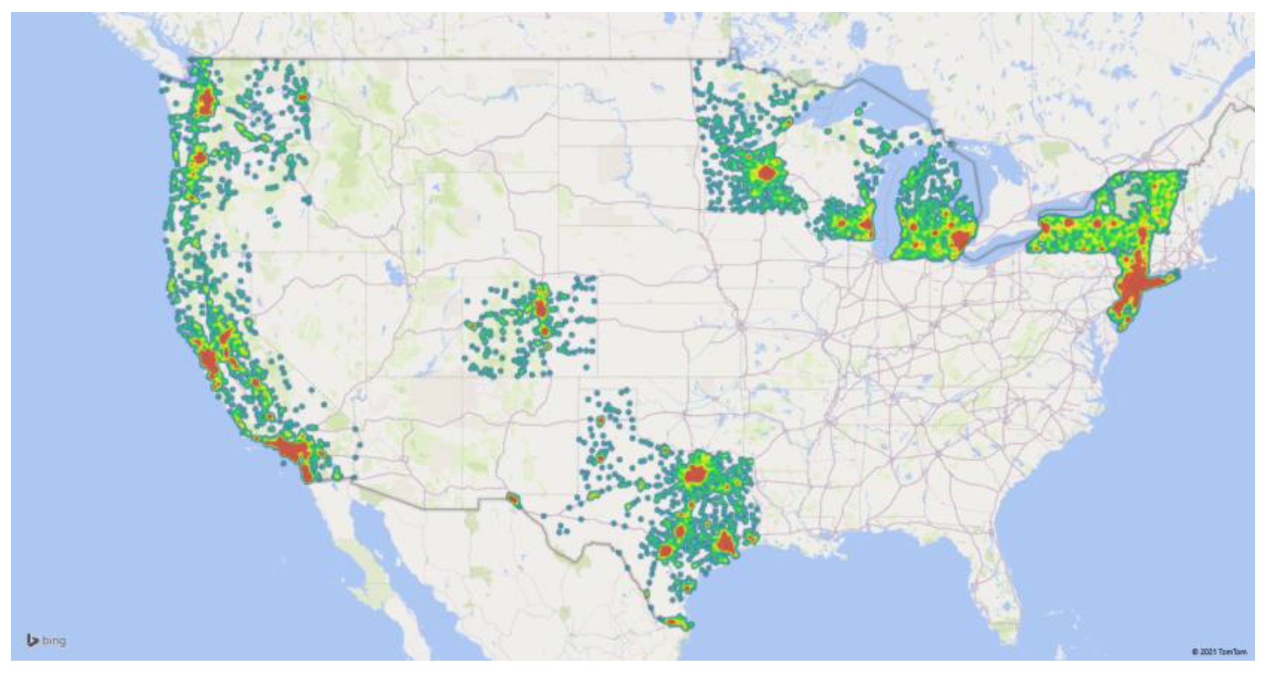
  • Examining 7155 ZIP codes across 11 states;
  • Developing a research framework to transform the granular demographic data into features more relevant to BEV uptake;
  • Quantifying the relationship between the demographic features and BEV uptake at different geographic locations.
Only BEV uptake is studied as opposed to plug-in hybrids because BEVs put forward greater challenges of range anxiety [35] and travel time, which can be consequential in understanding the demographic factors. The results from this study are relevant to several applications, including policymaking, charging infrastructure planning, and charging demand analysis, for example. In addition, the framework of this study can help to better understand the uptake of other vehicular technology, such as autonomous vehicles [36].
The paper is organized as follows: Section 2 discusses the description of the demographic features and BEV uptake, Section 3 discusses the engineering of the features and the correlation techniques used, and Section 4 discusses the results and their significance, followed by conclusions and future research opportunities.

2. Demographic Feature Analysis and BEV Uptake

BEV uptake is sparsely distributed across ZIP codes in all the 11 states studied. Uptake is highly skewed between states as well, with California leading the US. To understand the underlying factors responsible for this inconsistent distribution, both among the states and the ZIP codes within them, the socio-economic factors characterizing each region are quantified and analyzed.
Demographic features are used to characterize individual ZIP codes. These features are collected from an open resource of census data for the year 2019 [37]. From all the features in this dataset, all features falling under broad categories with a potential for affecting BEV uptake are initially considered. BEV uptake in a ZIP code is the target variable in this analysis. This is quantified as the number of BEVs registered with home addresses in a particular ZIP code at a specific time. BEV registration is selected over sales metrics, as it better captures the number of vehicles on the road and more accurately reflects the area of residence for each driver. In this study, records of BEV registrations for 11 states at the ZIP code level are used from available open resources [38,39]. The time frame for active BEV registrations is selected from February 2019 to February 2020. The data timeframe is chosen in part to exclude the impact of COVID-19, the effects of which can be examined by following a similar framework in future longitudinal studies.
The above data is collected for each ZIP code across 11 states. A total of 242 demographic characteristics potentially relevant to BEV uptake are initially selected for this study. Figure 2 shows a heatmap of BEV uptake in the 7155 ZIP codes considered in the 11 states in the US. ZIP codes are colored as a gradient from green (0 BEV) to red (5 or more BEVs).
Table 1 shows a summary table of the states considered with the number of ZIP codes in each state and the total BEVs. Additionally shown is the coarse distribution of BEVs within each state across ZIP codes. It is observed that the highest percentage of ZIP codes with “0” BEV registrations is Wisconsin, “1–99” BEV registrations is New Jersey, and “>100” BEV registrations is California.
Once the data is collected, it is preprocessed to maintain data consistency. The demographic data is processed based on the following considerations:
  • Population of a ZIP code, if zero, it is removed;
  • Any ZIP codes with “#N/A” or “-” values are removed. However, before eliminating the ZIP code, it is investigated if the discrepant values can be retrieved from other information in that ZIP code. As an example, if owner-occupied housing unit has “#N/A” value, it can be retrieved by subtracting rented-occupied housing units from total occupied housing units, if that information is available;
  • When features are reported as a percentage of the total population in the ZIP code, they are converted to an absolute number;
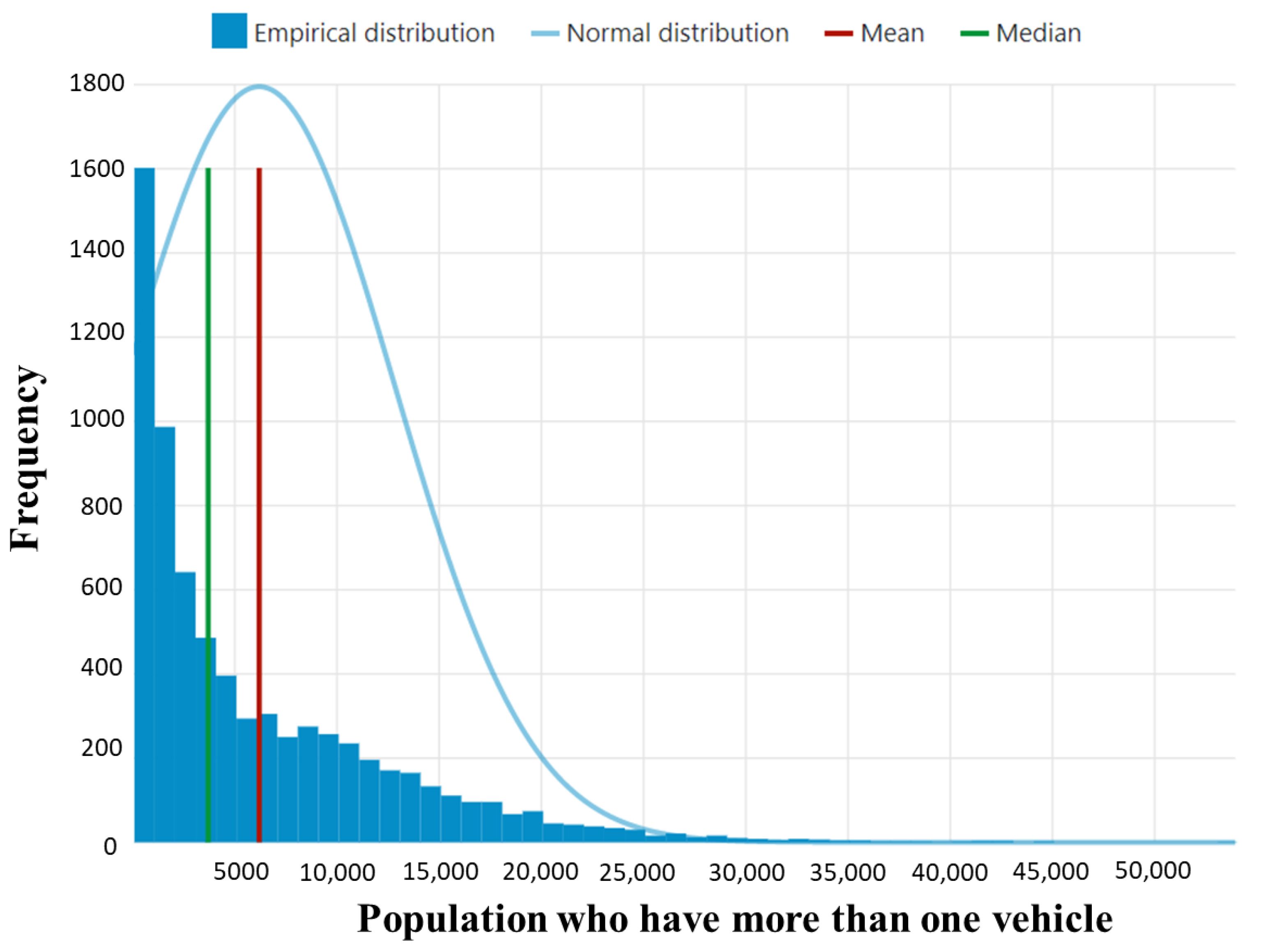
  • Median income in the ZIP codes is reported in a few cases as “25,000−” or “250,000+”. In both cases, the boundary values are the actual value, i.e., 25,000 and 250,000.
Understanding the demographic features: From all the demographic features available, 242 features that are hypothesized to impact BEV uptake are selected to characterize a location (ZIP code) for the selected state. These demographic features are organized into three classes based on whether the data is reported as individuals, housing units, or US dollars:
  • Class 1: Demographic features that provide information in terms of number of individuals;
  • Class 2: Demographic features that provide information in terms of the number of housing units;
  • Class 3: Demographic features that provide information in terms of income (in USD).
The demographic features are further classified into six broad categories based on the type of information they convey about the ZIP code:
  • Category 1—Population: Number of residents in the ZIP code. Typically helps us to understand BEV penetration with respect to the population of that place;
  • Category 2—Vehicle Information: Number of vehicles owned by individuals or households;
  • Category 3—Traveling Characteristics: Characterizes the traveling nature of the residents of the place, including means of transportation and average daily commute time;
  • Category 4—Migration of the Residents: Growth of the ZIP code in terms of residents moving out of the area or coming in;
  • Category 5—Economy: Financial information of the ZIP code;
  • Category 6—Living Arrangements: Owner-occupied and multi-dwelling units help to understand the type of housing units in which the residents reside.
Category 1–4 are expressed in terms of the number of individuals; Category 5 includes information on both number of individuals and income (USD), and Category 6 includes information on the number of housing units. One of the primary objectives of this study is to understand how each category of features affects BEV uptake and how some of the categories interact with each other to affect BEV uptake. For many of the demographic features in this study, the six categories overlap each other. The demographic features are then grouped based on their categories for further analysis. A total of 15 groups are formalized for this study. Table 2 shows the 242 demographic features studied and the group to which they belong. The table shows the categories of data within each group, the type of information, and the number of features fitting this description. An example from each group is provided for clarity.
The interaction of the categories is important to study along with the individual categories to better understand the complex factors contributing to BEV uptake. Many features provide information about the number of individuals or households that meet multiple simultaneous criteria, the intersection of which may affect BEV uptake more than either factor individually. In addition, many of the features contain excessively granular brackets of data that may not individually correlate well with BEV uptake. However, new features can be engineered from this information that better explain the BEV uptake in the ZIP code.

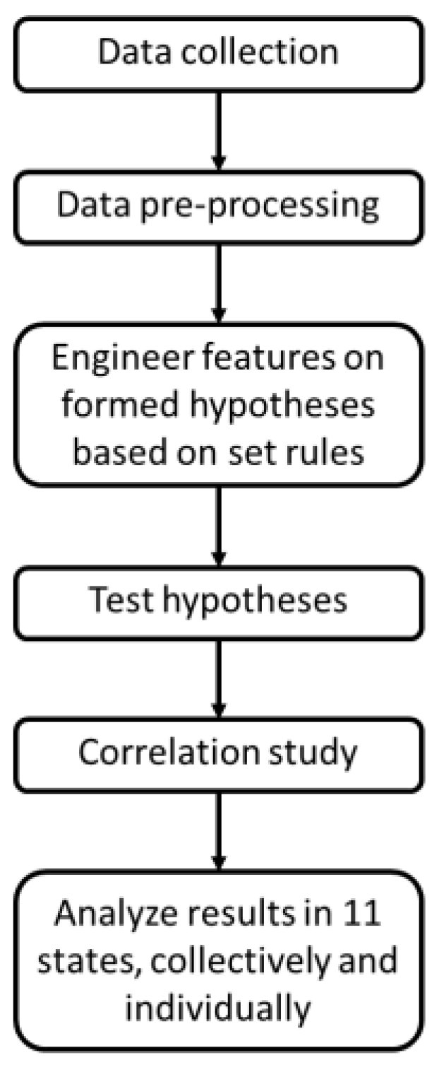
3. Demographic Feature Analysis and BEV Uptake

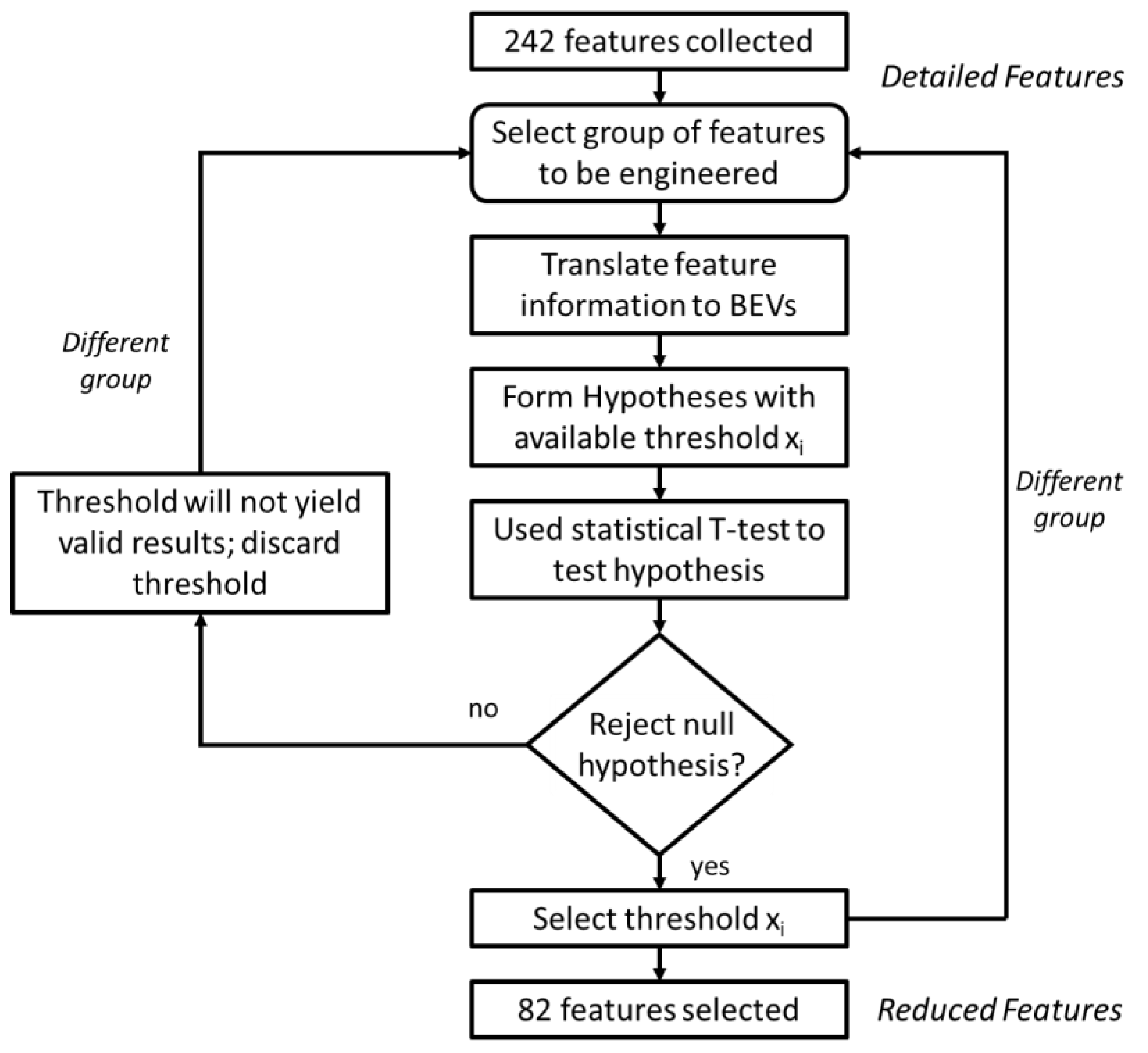
3.1. Feature Engineering and Selection

Feature engineering is commonly used by machine learning researchers to transform raw data to better understand the underlying problem at hand. Here, feature engineering helps to structure the raw data in such a manner to yield more meaningful information and provide a better understanding of BEV uptake.
While not all the original features may be well correlated with BEV uptake, useful information may still be extracted from the features. Formed hypotheses are used to engineer new features from available information. Features can then be selected to study their correlation with BEV uptake at the ZIP code level. In this paper, the initial 242 demographic features are hereafter referred to as Detailed Features. The Detailed Features are subjected to feature engineering and a final set of 82 features are then selected for the study that yields meaningful correlation results. This list of 82 features is hereafter referred as the Reduced Features. Detailed Features and Reduced Features follow the same structural framework, where the groups and categories remain the same and only the number of features in each group differ.
To determine the Reduced Features list, hypotheses are formulated against given thresholds to engineer features, which are tested using t-tests. To perform the t-tests, the demographic features are normalized in terms of BEV uptake. If the formed hypotheses hold true, the threshold is selected, and the number of features can be reduced based on the threshold. Otherwise, the threshold can be dismissed as it yields no statistically meaningful results. Figure 3 shows the flowchart of the process of generating the Reduced Features from the Detailed Features through hypothesis testing and threshold selection.
Each category is examined to form the hypotheses at certain thresholds. The formed hypotheses and their respective thresholds are as follows:
Hypothesis 1.
Travel time.
In the Detailed Features, the data for the average daily commute time are provided at 5–10 min intervals. The number of people within each small bracket of commute time may not correlate well with BEV uptake at the ZIP code level. Instead, it is hypothesized that individuals with a commute shorter than some threshold times may have a different likelihood of driving a BEV than individuals with a longer commute, potentially owing to range anxiety [4]. Accounting for the data available for each ZIP code, the price and range of the popular BEV models sold, and considering driving behavior and weather constraints [6], a threshold time of 60 min is hypothesized and tested.
Hypothesis 2.
Commuting characteristics.
For the Detailed Features, commuting characteristics are reported as the number of individuals with a given means of transportation to work. The available data specifies how many individuals commute to work using a car and driving alone, in a 2/3/4 or more person carpool, or by public transportation, bicycle, or other means. In the granulated form, the correlation significance for a single feature in this context can be minimal when studying BEV uptake. The hypothesis is made that the number of people in a carpool, or the type of alternate transportation, are not relevant to BEV uptake. The engineered features are thus grouped based on the number of people driving alone, carpooling, or using other means of transportation.
Hypothesis 3.
Number of vehicles.
In the Detailed Features group, the number of vehicles is reported for a household as well as for an individual in terms of 0/1/2/3/4/5, or more. Correlation between each exact number of vehicles present can be of low significance to the BEV uptake. For a better understanding of the number of vehicles present and its relationship with BEV uptake, a hypothesis is made that an individual or household’s likelihood to buy a BEV may depend on whether they own zero, one, or more than one vehicle.
Hypothesis 4.
Types of housing-unit structures.
For the Detailed Features, types of housing-unit structures are reported in increments of occupants, such as 1/2/(3–4)/(5–9), and up to 50 or more. In a broader sense, types of housing-unit structures help us to understand whether an individual lives in a single-dwelling unit or a multi-dwelling unit. This level of granularity in the case of the multi-dwelling units is hypothesized to not be significant with respect to BEV uptake. For the engineered features, this data is simplified to the number of individuals living in single-dwelling units and the number of individuals living in multi-dwelling units.
Hypothesis 5.
Income level.
For the Detailed Features, the income of an individual is reported in USD from no income to USD 150 k and above in non-uniform intervals. It is intuitive that the higher the income of an individual or household, the more likely they are to purchase a BEV. However, small income brackets will not individually correlate well with any target variable. It is hypothesized that the likelihood to buy an EV is affected by whether an individual has some threshold of disposable income. Comparing the price and ranges of popular sold models in the US with a federal discount and maintenance annually [40], it is observed that a BEV costs approximately USD 23 k on average. From national data and surveys, it is recommended that the price of an individual’s car should be 30% of their annual income [41]. With this information, and the available income brackets in the ZIP code data, income features in the Reduced Features are calculated based on the numbers of individuals making more or less than USD 75 k annually.
The formed hypotheses discussed need to be statistically tested to establish the validity of the thresholds set. The t-test is used for testing all the formed hypotheses. The steps to engineer and select the 82 features from the 242 features are shown in Algorithm 1.
Algorithm 1:t-tests to test the hypotheses to engineer the features
1242 Detailed Features are collected.
2Select group j where features are to be engineered, where j = 1, 2, …., n = 15.
The details of group j are shown in Table 2.
3Form hypothesis for group j, based on available threshold xi
4For group j, demographic data is translated to BEV uptake information.
Class 1: Average BEVs per population
Class 2: Average BEVs per housing units
Class 3: No thresholds can be set, and hypothesis testing is not required.
5Form null and alternate hypothesis.
Null hypothesis (Ho): Threshold will not affect BEV uptake.
Alternate hypothesis (Ha): Threshold will affect BEV uptake, and threshold xi is selected for analysis.
6Determine tcalculated.
t c a l c u l a t e d = x ¯ 1 x ¯ 2 σ 1 2 n 1 + σ 2 2 n 2 ,
Where ,   x ¯ 1 , x ¯ 2   = observed mean of the two samples,
σ 1 2 , σ 2 2 = variance of the two samples
n 1 , n 2 = Sample 1 and 2
7Determine degrees of freedom (df).
Df = sample size (k) – 2
8j = j + 1, if j ≤ 15.
If tcalculated > tcritical, reject Ho. Select xi. Go to Step 3.
Else, discard group for analysis. Go to Step 3.
9Select the Reduced Features from successful t-tests.

3.2. Correlation Study

The Reduced Features represent the most statistically significant version of the information available in the original dataset but must be further studied to determine if there is a meaningful correlation with BEV uptake in each of the zip codes. Correlation studies are performed on individual states and for the 11 states, collectively. Spearman’s coefficient is used for the correlation study, as the data is non-Gaussian. To test Gaussian distribution, D’Agostino’s test [42] is used. To illustrate the non-Gaussian nature of the demographic features, the histogram plot for an example feature is shown in Figure 4, showing the population that owns more than one vehicle [43]. The skewness-kurtosis test has a value of 2238 and the p-value is less than α = 0.05. This suggests that the data distribution is not normal. While only one example is shown, all demographic features in the Detailed and Reduced Features sets are tested and exhibit similar non-Gaussian distributions.
Spearman’s correlation coefficients can range from “−1” to “1”, with “−1” indicating perfect negative correlation, “0” indicating no correlation, and “1” indicating perfect positive correlation between a demographic feature and BEV uptake. For subsequent qualitative comparisons of the strength of each Spearman’s coefficient, it is posited that “weak correlation” corresponds to coefficients below 0.6, “fair correlation” to coefficients between 0.6 and 0.8, and “strong correlation” to coefficients above 0.8 [44].

4. Results and Discussion

In this section, partial results from the study are shown, including feature engineering, hypothesis testing, feature selection, and correlation analysis. The correlation study not only helps to understand how features are correlated with BEV uptake, but the study also helps to validate the engineering of the features. In this paper, due to space limitations, not all the results are shown. To demonstrate the conducted work, several examples are given in detail, followed by a summary of the correlation results across both states and feature categories.
Features containing information about the income of the population in a ZIP code (Group 5) are used to demonstrate the proposed research framework. Hypotheses formed for this group are discussed and results of hypothesis testing are shown. The correlation results for this group are shown for both Detailed Features and Reduced Features, and for individual states, and all the states collectively. Next, features containing information about the means of transportation of the population in the ZIP code (part of Group 3) are discussed. To illustrate the feature interaction and its importance, Group 8 is discussed next, which contains information about the combination of income and means of transportation. From the complete set of 82 Reduced Features, the 10 best correlated features are presented for all of 11 states, individually and collectively. Finally, the best feature from each group is shown to illustrate the extent of correlation of these groups with BEV uptake.
This section may be divided by subheadings. It should provide a concise and precise description of the experimental results, their interpretation, as well as the experimental conclusions that can be drawn.

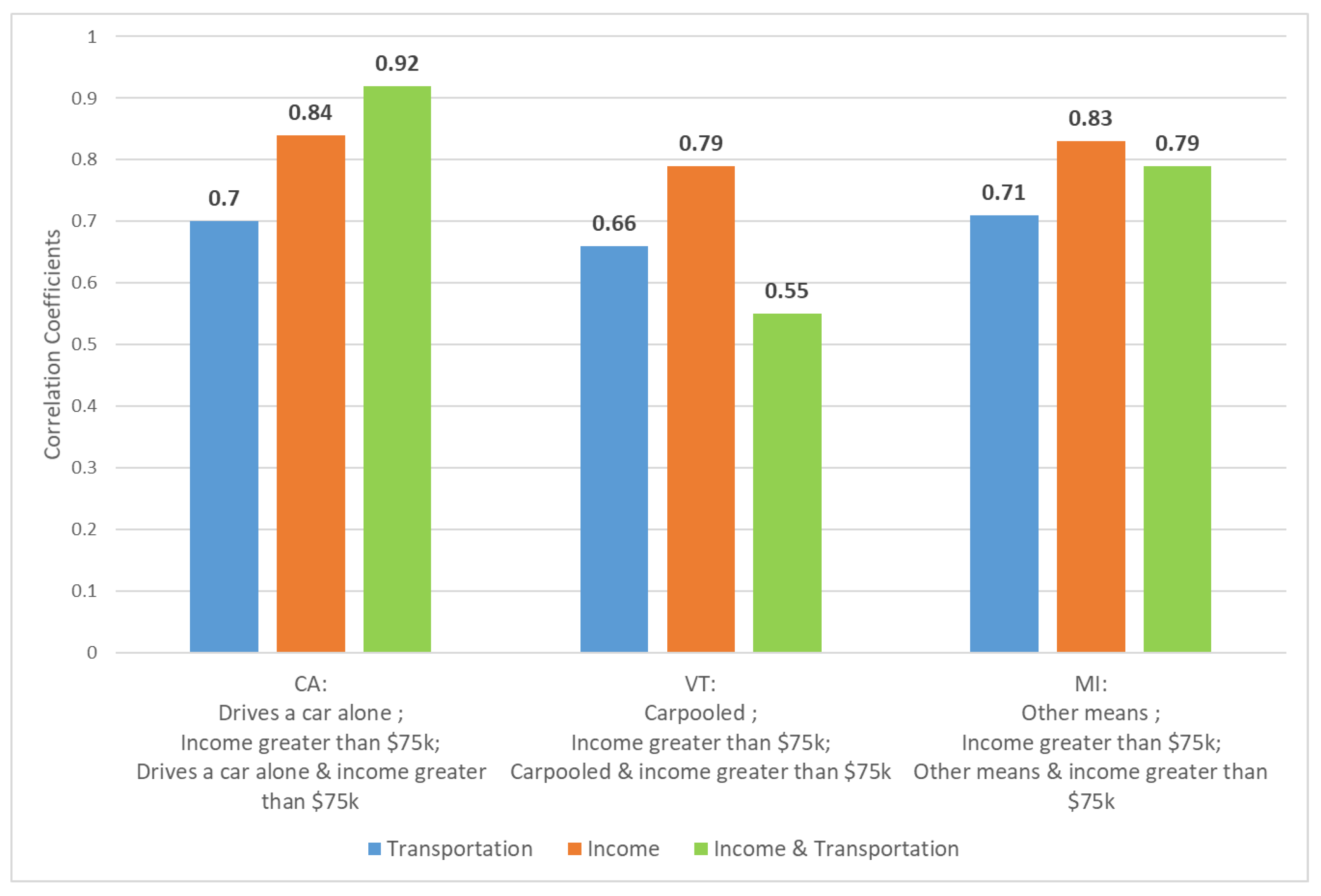
4.1. Understanding the Research Framework Using Features of Income, Means of Transportation, and Both

4.1.1. Characterization of ZIP Codes in Terms of Income

Group 5 contains information about the income of individuals in the ZIP code. The original data collected have eight features, and the income bracket columns are shown in Table 3.
The formulated hypothesis for income level is that the relevant threshold is USD 75,000. Based on the set threshold, data is calculated based on the population having an income less than USD 75,000 and the population having an income greater than USD 75,000 in a ZIP code.
P o p . I n c o m e < U S D   75 , 000 = I n c o m e   b r a c k e t = a g I n c o m e C o l u m n
For hypothesis testing, first, the values are transformed into average population per BEV. Null and alternate hypotheses are formed.
Null Hypothesis: The average population per BEV with an income greater than USD 75,000 is the same as the average population per BEV with an income less than USD 75,000.
Alternate Hypothesis: The average population per BEV with an income greater than USD 75,000 is different than the average population per BEV with an income less than USD 75,000.
For conducting hypothesis testing, the t-test is used. The tcritical is determined to be 1.96 for degrees of freedom greater than 100 [45]. The t is calculated for all the 11 states and the states individually. Results are given in Table 4.
As tcalculated is greater than tcritical, the null hypothesis is rejected. This means that the average population per BEV is different depending on income brackets. Once it is established that the alternate hypothesis is true, the correlation of the income features to BEV uptake is investigated, and the results are shown in Table 5. The table includes Detailed Features and Reduced Features for all of the 11 states and for each state individually. The Spearman correlation coefficients are studied to analyze whether and by what degree the engineered features present meaningful results.
From Table 5, it is evident that income brackets USD 1 to USD 9999 and USD 35,000 to USD 49,999 have a similar degree of correlation, whereas the income brackets between them are different. However, the population with an income greater than USD 75,000 has a greater correlation with BEV uptake than the population with an income less than USD 75,000. This holds true for all the 11 states collectively and individually. In Colorado, Oregon, and Washington, though there is a degree of difference in the correlation coefficients, both brackets are strongly correlated with the BEV uptake.

4.1.2. Characterization of ZIP Codes in Terms of Means of Transportation

Group 3 contains the information about the means of transportation of the individuals in the ZIP code. Table 6 shows the Detailed Features and Reduced Features for Group 3. For this group, the commuting characteristic hypothesis is implemented to engineer features. Reduced Features are based on the population who drives a car alone, carpools, or uses other means to travel to work. Other means of travel include public transportation, bicycles, walking, using taxicabs, or working from home.
From Table 6, it is observed that the Detailed Features exhibit varying degrees of correlation individually. It is also observed that the population who are working from home has a strong correlation with BEV uptake. In the Reduced Features for this group, it is seen that the population who drives a car alone, carpooled, or used other means, each has a moderate correlation with BEV uptake, with small differences in the degree of correlation.

4.1.3. Characterization of ZIP Codes in Terms of Income and Means of Transportation

To study how the features interact and if the interaction of these features has an impact on their correlation with BEV uptake, Group 8 is studied. Group 8 contains information about the intersection of features in Groups 3 and 5. Specifically, these features report the number of individuals with both a given commuting behavior and income level. The thresholds established for income and commuting are used to engineer the features for this group. An example of such an engineered feature is the population in a ZIP code who drives a car alone and has an income greater than USD 75,000. Table 7 shows the correlation results for Group 8 with BEV uptake for all the states and each state individually.
From Table 7, it is seen that for all the states collectively, the number of individuals having an income greater than USD 75,000 and driving alone or traveling using other means has a greater degree of correlation than the rest of the features. Most of the states exhibit the same trend, with New Jersey displaying the starkest example. In Colorado, Minnesota, and Wisconsin, the correlation of all six features is more similar.
Features describing the number of individuals that meet multiple criteria often exhibit a stronger correlation with BEV uptake than the single criteria feature they correspond to, but this is not always the case. Figure 5 is a bar graph showing a sample of such interactions across different features and states. It is observed that features containing composite criteria can correlate very differently from features containing only part of the same information. In California, among the population driving a car alone, or having income greater than USD 75,000, each has a moderate to strong correlation with BEV uptake. However, the number of individuals meeting both criteria has a very strong correlation. Conversely, in Vermont, the population who carpools and the population with an income greater than USD 75,000 each have moderate correlation with BEV uptake, but the feature describing the intersection of these criteria is weakly correlated. Lastly, in Michigan, there is not a large difference in correlation between the population traveling by other means, the population with an income greater than USD 75,000, and the population meeting both criteria.

4.2. The 10 Best Correlated Features with BEV Uptake

An extensive study is performed with the Reduced Features, consisting of 82 demographic features in total, across all 15 groups with BEV uptake, for each of the 11 states individually and collectively. The 10 best correlated features are shown in Table 8, based on the results from the collective data of 11 states. The green boxes indicate strong correlation, the red indicate moderate correlation, and the white indicate weak correlation, as defined in Section 3.
The 10 best demographic features include three features from Group 13 (information on living arrangements and economy), two features from Group 8 (income and means of transportation), and one feature each from Groups 3 (means of transportation), 5 (economy), 7 (means of transportation and vehicles), 10 (living arrangement and means of transportation), and 11 (migration and economy). A total of 7 out of 10 features have information that relates to the population with an income greater than USD 75,000. It is noted that despite correlating well across the 7155 ZIP codes, two of the features have a weak correlation within individual states. In most cases, however, the top 10 features are similar for the unified model and in each state individually, though the degree of correlation with the BEV uptake varies. Table 9 shows the summary of the top 10 features and which states have those features in their top 10 list as well. Additionally, the average ranking of the features is shown to demonstrate the relative variability of these features among the states.

4.3. The Best Correlated Feature of Each Group

The best feature from each group is shown in Table 10. Analyzing the best feature from each group provides a summary of how well this type of information correlates with BEV uptake in a ZIP code. The “best” feature is determined based on the unified model of all states, but its performance is shown for each state individually as well. It is noted that for almost all the states, the selected feature for each group is also the best in the individual state model; however, the value of their correlation can differ significantly.
Figure 6 shows a final qualitative summary of the correlation study for the Reduced Features set. For the unified model of 11 states, there are five features with a strong correlation with BEV uptake. At the individual state level, Vermont and Wisconsin do not have any features with strong correlation. In contrast, half of the studied features are strongly correlated with BEV uptake in Colorado, Washington, and Oregon. A total of 22 of the 82 Reduced Features in the unified model are weakly correlated with BEV uptake. In the state models, most features in New Jersey, Vermont, and Wisconsin are weakly correlated. Finally, in most of the states and in the unified model, more than half of the selected features are moderately correlated with BEV uptake in a ZIP code.

4.4. Discussion of Results

Many of the demographic factors studied exhibit a moderate to strong correlation with BEV uptake. While most demographic features are themselves correlated with the population in a ZIP code, features which quantify more specific subsets of the population often correlate more strongly with BEV uptake. Many of the above results confirm common intuitions, such as the fact that seven of the top 10 features quantify subsets of the population with an income greater than USD 75 k. It is important in any correlation analysis, however, to note that these relationships cannot be assumed to be causal—the population fitting the description of well-correlated demographic features is not necessarily the only population purchasing BEVs. The demographic factors are simply aggregate descriptors of the ZIP code as a whole.
Importantly, the strength of correlation for the various demographic factors is not static across states. In New Jersey, the majority of demographic features are weakly correlated with BEV uptake, whereas in Oregon the majority of demographic features are strongly correlated. It is observed that when the average number of BEVs per ZIP code in a state is higher, there is a stronger correlation between demographic factors and BEV uptake, evidenced in Colorado, Oregon, and Washington. California, with the highest average number of BEVs per ZIP code, performs very similarly to the full 11-state model. It is also inferred that lower BEV adoption in a state can cause demographic factors to be more weakly correlated with BEV uptake. Vermont and Wisconsin do not have any strongly correlated demographic factors, and their overall BEV adoption is very low.
In addition, certain important non-demographic factors, including charging infrastructure, EV incentives, and fuel and electricity prices can vary significantly between states. These factors not only affect BEV uptake directly but can change the relationship between demographic factors and BEV uptake. The relative consistency in performance in the best correlated features, however—as well as the large number of moderately to strongly correlated features in the 11-state model—show that quantitative knowledge on the financial characteristics, commuting features, living arrangements, and migration of residents in a ZIP code can explain much of the variance in BEV adoption.

5. Conclusions

In this paper, an extensive study is conducted to study the correlation of demographic factors with BEV uptake at a granular level at a larger scale. A total of 242 demographic features are collected at the ZIP code level and preprocessed to maintain data consistency. The features are categorized based on the type of information they provide, including population, vehicle information, traveling characteristics, economy, housing, and migration information. New features are then engineered, forming certain hypotheses to set the thresholds, which are validated using t-tests.
Of the demographic features studied, it is determined that the number of individuals in a ZIP code having income greater than USD 75,000 has the strongest correlation with BEV uptake overall. Of other features of interest, the number of owned housing units has a greater correlation with BEV uptake than rented housing units. With respect to means of transportation, both the number of individuals who drive to work alone or by other means of transportation are well correlated with BEV uptake. The number of individuals who are working from home appears to be contributing most of the correlation for other means of transportation.
These factors, as well as others listed in Table 8, Table 9 and Table 10, represent the demographic descriptors of a ZIP code, which are most correlated with local BEV uptake, rather than descriptors of individual BEV purchasers. Understanding such aggregate factors at the local level is thus important for the effective prediction and accommodation of accelerating BEV uptake across socio-demographically disparate areas.
For future work, a regression model will be developed to analyze these demographic features and better understand BEV uptake at the ZIP code level. While correlation analysis helps to assess each feature’s univariate relationship to the dependent variable, regression can address the co-dependency and multicollinearity of the independent variables and their effect on BEV uptake in a ZIP code.

Author Contributions

Conceptualization, S.S. and K.J.; methodology, S.S. and K.J.; software, S.S.; validation, S.S., K.J. and M.A.; formal analysis, S.S. and K.J.; investigation, S.S.; resources, S.S.; data curation, S.S.; writing—original draft preparation, S.S. and K.J.; writing—review and editing, K.J. and M.A.; visualization, S.S.; supervision, M.A.; project administration, M.A.; funding acquisition, M.A. All authors have read and agreed to the published version of the manuscript.

Funding

This research was funded by the Nebraska Environmental Trust (NET), the Nebraska Community Energy Alliance (NCEA), and the Durham School of Architectural Engineering and Construction—University of Nebraska–Lincoln.

Institutional Review Board Statement

Not applicable.

Informed Consent Statement

Not applicable.

Conflicts of Interest

The authors declare no conflict of interest.

References

  1. Power, J.D. How Does the Federal Tax Credit for Electric Cars Work? Available online: https://www.jdpower.com/cars/shopping-guides/how-does-the-federal-tax-credit-for-electric-cars-work (accessed on 29 November 2021).
  2. Zhang, Q.; Li, H.; Zhu, L.; Campana, P.E.; Lu, H.; Wallin, F.; Sun, Q. Factors influencing the economics of public charging infrastructures for EV—A review. Renew. Sustain. Energy Rev. 2018, 94, 500–509. [Google Scholar] [CrossRef]
  3. Shi, L.; Hao, Y.; Lv, S.; Cipcigan, L.; Liang, J. A comprehensive charging network planning scheme for promoting EV charging infrastructure considering the Chicken-Eggs dilemma. Res. Transp. Econ. 2020, 88, 100837. [Google Scholar] [CrossRef]
  4. Shom, S.; Al Juheshi, F.; Rayyan, A.; Abdul-Hafez, M.; Shuaib, K.; Alahmad, M. Characterization of a search algorithm to determine number of electric vehicle charging stations between two points on an Interstate or US-Highway. In Proceedings of the 2017 IEEE Transportation Electrification Conference and Expo (ITEC), Chicago, IL, USA, 22–24 June 2017; pp. 690–695. [Google Scholar] [CrossRef]
  5. Shom, S.; Alahmad, M. Determining optimal locations of electrified transportation infrastructure on interstate/ us-highways. In Proceedings of the 2017 13th International Conference and Expo on Emerging Technologies for a Smarter World (CEWIT), Stony Brook, NY, USA, 7–8 November 2017; pp. 1–7. [Google Scholar] [CrossRef]
  6. Shom, S.; Guha, A.; Alahmad, M. Ruler-Search Technique (RST) Algorithm to Locate Charging Infrastructure on a Particular Interstate or US-Highway. In Proceedings of the 2018 IEEE Transportation Electrification Conference and Expo (ITEC), Long Beach, CA, USA, 13–15 June 2018; pp. 326–331. [Google Scholar] [CrossRef]
  7. Shom, S.; Al Juheshi, F.; Rayyan, A.; Alahmad, M.; Abdul-Hafez, M.; Shuaib, K. Case studies validating algorithm to determine the number of charging station placed in an Interstate and US-Highway. In Proceedings of the 2017 IEEE International Conference on Electro Information Technology (EIT), Lincoln, NE, USA, 14–17 May 2017; pp. 050–055. [Google Scholar] [CrossRef]
  8. Alternative Fuels Data Center: Alternative Fueling Station Locator. Available online: https://afdc.energy.gov/stations/#/find/nearest?country=US&fuel=ELEC&location=nebraska (accessed on 13 December 2021).
  9. Zhou, Y.; Wen, R.X.; Wang, H.W.; Cai, H. Optimal battery electric vehicles range: A study considering heterogeneous travel patterns, charging behaviors, and access to charging infrastructure. Energy 2020, 197, 116945. [Google Scholar] [CrossRef]
  10. Pagany, R.; Camargo, L.R.; Dorner, W. A review of spatial localization methodologies for the electric vehicle charging infrastructure. Int. J. Sustain. Transp. 2018, 13, 433–449. [Google Scholar] [CrossRef] [Green Version]
  11. Straka, M.; De Falco, P.; Ferruzzi, G.; Proto, D.; Van Der Poel, G.; Khormali, S.; Buzna, L. Predicting Popularity of Electric Vehicle Charging Infrastructure in Urban Context. IEEE Access 2020, 8, 11315–11327. [Google Scholar] [CrossRef]
  12. AlMaghrebi, A.; AlJuheshi, F.; Rafaie, M.; James, K.; Alahmad, M. Data-Driven Charging Demand Prediction at Public Charging Stations Using Supervised Machine Learning Regression Methods. Energies 2020, 13, 4231. [Google Scholar] [CrossRef]
  13. Li, C.; Dong, Z.; Chen, G.; Zhou, B.; Zhang, J.; Yu, X. Data-Driven Planning of Electric Vehicle Charging Infrastructure: A Case Study of Sydney, Australia. IEEE Trans. Smart Grid 2021, 12, 3289–3304. [Google Scholar] [CrossRef]
  14. Kumar, R.R.; Alok, K. Adoption of electric vehicle: A literature review and prospects for sustainability. J. Clean. Prod. 2020, 253, 119911. [Google Scholar] [CrossRef]
  15. Priessner, A.; Sposato, R.; Hampl, N. Predictors of electric vehicle adoption: An analysis of potential electric vehicle drivers in Austria. Energy Policy 2018, 122, 701–714. [Google Scholar] [CrossRef]
  16. Chen, C.-F.; de Rubens, G.Z.; Noel, L.; Kester, J.; Sovacool, B.K. Assessing the socio-demographic, technical, economic and behavioral factors of Nordic electric vehicle adoption and the influence of vehicle-to-grid preferences. Renew. Sustain. Energy Rev. 2020, 121, 109692. [Google Scholar] [CrossRef]
  17. Lin, B.; Wu, W. Why people want to buy electric vehicle: An empirical study in first-tier cities of China. Energy Policy 2018, 112, 233–241. [Google Scholar] [CrossRef]
  18. Zhuge, C.; Shao, C. Investigating the factors influencing the uptake of electric vehicles in Beijing, China: Statistical and spatial perspectives. J. Clean. Prod. 2018, 213, 199–216. [Google Scholar] [CrossRef] [Green Version]
  19. Sovacool, B.K.; Abrahamse, W.; Zhang, L.; Ren, J. Pleasure or profit? Surveying the purchasing intentions of potential electric vehicle adopters in China. Transp. Res. Part A Policy Pract. 2019, 124, 69–81. [Google Scholar] [CrossRef]
  20. Karlberg, C. The Survey Fatigue Challenge: Understanding Young People’s Motivation to Participate in Survey Research Studies. Master’s Thesis, Lund University, Lund, Sweden, June 2015; p. 27. [Google Scholar]
  21. Wee, S.; Coffman, M.; Allen, S. EV driver characteristics: Evidence from Hawaii. Transp. Policy 2020, 87, 33–40. [Google Scholar] [CrossRef]
  22. Who are driving electric vehicles? An—ourenergypolicy. Available online: http://www.ourenergypolicy.org/wp-content/uploads/2018/06/Hawaii-EVs.pdf (accessed on 17 December 2021).
  23. Araújo, K.; Boucher, J.L.; Aphale, O. A clean energy assessment of early adopters in electric vehicle and solar photovoltaic technology: Geospatial, political and socio-demographic trends in New York. J. Clean. Prod. 2019, 216, 99–116. [Google Scholar] [CrossRef]
  24. Javid, R.J.; Nejat, A. A comprehensive model of regional electric vehicle adoption and penetration. Transp. Policy 2017, 54, 30–42. [Google Scholar] [CrossRef]
  25. Vergis, S.; Chen, B. Comparison of plug-in electric vehicle adoption in the United States: A state by state approach. Res. Transp. Econ. 2015, 52, 56–64. [Google Scholar] [CrossRef]
  26. Mukherjee, S.C.; Ryan, L. Factors influencing early battery electric vehicle adoption in Ireland. Renew. Sustain. Energy Rev. 2019, 118, 109504. [Google Scholar] [CrossRef]
  27. Gray, N.; Chalmers, R.; Gilbert, C. Data-driven EV uptake modelling. CIRED-Open Access Proc. J. 2020, 2020, 266–269. [Google Scholar] [CrossRef]
  28. Wicki, M.; Brückmann, G.; Quoss, F.; Bernauer, T. What do we really know about the acceptance of battery electric vehicles?—Turns out, not much. Transp. Rev. 2022, 1–26. [Google Scholar] [CrossRef]
  29. Yang, J.; Chen, F. How are social-psychological factors related to consumer preferences for plug-in electric vehicles? Case studies from two cities in China. Renew. Sustain. Energy Rev. 2021, 149, 111325. [Google Scholar] [CrossRef]
  30. Danielis, R.; Giansoldati, M.; Rotaris, L. A probabilistic total cost of ownership model to evaluate the current and future prospects of electric cars uptake in Italy. Energy Policy 2018, 119, 268–281. [Google Scholar] [CrossRef]
  31. Kabir, M.E.; Assi, C.; Alameddine, H.; Antoun, M.; Yan, J. Demand-Aware Provisioning of Electric Vehicles Fast Charging Infrastructure. IEEE Trans. Veh. Technol. 2020, 69, 6952–6963. [Google Scholar] [CrossRef]
  32. Kabir, M.E.; Assi, C.; Alameddine, H.; Antoun, J.; Yan, J. Demand Aware Deployment and Expansion Method for an Electric Vehicles Fast Charging Network. In Proceedings of the 2019 IEEE International Conference on Communications, Control, and Computing Technologies for Smart Grids (SmartGridComm), Beijing, China, 21–23 October 2019; pp. 1–7. [Google Scholar] [CrossRef]
  33. Antoun, J.; Kabir, M.E.; Atallah, R.F.; Assi, C. A Data Driven Performance Analysis Approach for Enhancing the QoS of Public Charging Stations. IEEE Trans. Intell. Transp. Syst. 2021, 1–10. [Google Scholar] [CrossRef]
  34. Shom, S.; James, K.; Alahmad, M. Correlation study between features of a geographic location and Electric Vehicle Uptake. In Proceedings of the 2021 IEEE Transportation Electrification Conference & Expo (ITEC), Anaheim, CA, USA, 21–25 June 2021; pp. 567–572. [Google Scholar] [CrossRef]
  35. Noel, L.; de Rubens, G.Z.; Sovacool, B.K.; Kester, J. Fear and loathing of electric vehicles: The reactionary rhetoric of range anxiety. Energy Res. Soc. Sci. 2018, 48, 96–107. [Google Scholar] [CrossRef]
  36. Hardman, S.; Berliner, R.; Tal, G. Who will be the early adopters of automated vehicles? Insights from a survey of electric vehicle owners in the United States. Transp. Res. Part D Transp. Environ. 2018, 71, 248–264. [Google Scholar] [CrossRef]
  37. Bureau, U.C.; Demographic Data. Census.Gov. Available online: https://www.census.gov/programs-surveys/ces/data/restricted-use-data/demographic-data.html (accessed on 17 December 2021).
  38. Atlas EV Hub. 2021. State EV Registration Data. Available online: https://www.atlasevhub.com/materials/state-ev-registration-data/ (accessed on 21 January 2022).
  39. Data.ca.gov. 2021; Vehicle Fuel Type Count By Zip Code—California Open Data. Available online: https://data.ca.gov/dataset/vehicle-fuel-type-count-by-zipcode (accessed on 21 January 2022).
  40. Federal Tax Credits for Electric and Plug-in Hybrid Cars. Fueleconomy.Gov. 2021. Available online: https://www.fueleconomy.gov/feg/taxevb.shtml (accessed on 21 January 2022).
  41. How Much Should You Spend On A Car? Money Under 30. 2021. Available online: https://www.moneyunder30.com/how-much-car-can-you-afford (accessed on 21 January 2022).
  42. Das, K.R. A Brief Review of Tests for Normality. Am. J. Theor. Appl. Stat. 2016, 5, 5. [Google Scholar] [CrossRef] [Green Version]
  43. GeorgiGeorgiev-Geo. Normality Test Calculator—Shapiro-Wilk, Anderson-Darling, Cramer-von Mises & more. Available online: https://www.gigacalculator.com/calculators/normality-test-calculator.php (accessed on 17 December 2021).
  44. Statstutor.ac.uk. 2021. Available online: https://www.statstutor.ac.uk/resources/uploaded/spearmans.pdf (accessed on 21 January 2022).
  45. Student’s T Critical Values. Available online: https://people.richland.edu/james/lecture/m170/tbl-t.html (accessed on 21 January 2022).
Figure 1. Flowchart showing the workflow.
Sustainability 14 05016 g001
Figure 2. Heatmap of US showing the BEV uptake in 7155 ZIP codes in the 11 states [38,39].
Sustainability 14 05016 g002
Figure 3. Flowchart showing the feature engineering process.
Sustainability 14 05016 g003
Figure 4. Histogram plot showing population with more than one vehicle, illustrating the highly non-normal distribution of a typical demographic feature [43].
Sustainability 14 05016 g004
Figure 5. Bar chart showing comparison of feature interactions.
Sustainability 14 05016 g005
Figure 6. Summary of the correlation study of 82 Reduced Features in all 11 states.
Sustainability 14 05016 g006
Table 1. Summary of the ZIP codes with BEV information.
Number of ZIP CodesTotal BEVs
Total“0” BEVs“1–99” BEVs“100–999” BEVs“>1000” BEVs
11 States715510545028102449455,352
Percentages of the Total ZIP Codes (%)
California14426.1044.8745.773.26302,966
Colorado34414.5368.0217.440.0017,012
Michigan71928.0971.350.560.005187
Minnesota49819.6878.511.810.007066
New Jersey5092.7588.029.230.0018,213
New York123311.6086.621.780.0021,822
Oregon29710.1068.0121.550.3422,441
Texas123722.3173.244.450.0022,495
Vermont18020.0078.891.110.001519
Washington4267.5168.5423.710.2335,648
Wisconsin27031.4868.520.000.00983
Table 2. Demographic features description (Gr: group).
GrCategories and Their InteractionType of InformationNumber of FeaturesExample
1Population (Category 1)#Individuals2Total population older than 16 years old
2Vehicle Information (Category 2)#Individuals6Total population with one vehicle
3Traveling Characteristics (Category 3)#Individuals25Total population that commutes less than 5 min daily
4Migration of Residents (Category 4)#Individuals4Total population that moved from different state
5Economy (Category 5)#Individuals8Total population that earns less than USD 10,000
6Living Arrangements (Category 6)#Housing units13Total multi-dwelling housing units
7Category 2, 3#Individuals24Total population that drives alone and owns one vehicle
8Category 3, 5#Individuals24Total population that drives alone and earns less than USD 10,000
9Category 1, 3#Individuals27Total population that drives alone and less than 10 min daily
10Category 1, 3, 6#Individuals6Total population that drives alone and lives in rented housing
11Category 4, 5#Individuals32Total population that moved from different state and earns less than USD 10,000
12Category 1, 6#Individuals2Total population living in rented housing
13Category 6, 5#Housing units55Total owner-occupied housing earning less than USD 10,000
14Category 6, 2#Housing units12Total owner-occupied housing where occupants have one vehicle
15Category 6, 5#Income (USD)2Median income of occupants of owner-occupied housing
Table 3. Income brackets of the Detailed Features.
Income BracketDescription
(a)USD 1 to USD 9999
(b)USD 10,000 to USD 14,999
(c)USD 15,000 to USD 24,999
(d)USD 25,000 to USD 34,999
(e)USD 35,000 to USD 49,999
(f)USD 50,000 to USD 64,999
(g)USD 65,000 to USD 74,999
(h)USD 75,000 and more
Table 4. The t-tests results for the 11 states collectively and individually.
t-Calculatedt-Critical
11 states35.21.96
CA17.46
CO9.49
MI14.9
MN15
NJ9.22
NY17.83
OR11.15
TX19.48
VT8.51
WA10.65
WI10.08
Table 5. Correlation results for income group without and with feature engineering in 11 states.
Population with IncomeSpearman Correlation Coefficient
11 statesCACOMIMNNJNYORTXVTWAWI
Detailed FeaturesUSD 1 to USD 99990.660.590.810.700.790.450.730.860.650.710.800.63
USD 10,000 to USD 14,9990.630.530.790.660.760.350.700.840.600.660.770.60
USD 15,000 to USD 24,9990.620.510.790.670.750.310.680.850.600.630.740.60
USD 25,000 to USD 34,9990.630.540.790.670.760.330.680.870.640.670.750.59
USD 35,000 to USD 49,9990.660.620.820.710.780.370.710.870.710.670.800.63
USD 50,000 to USD 64,9990.720.730.850.760.800.470.770.890.790.690.840.67
USD 65,000 to USD 74,9990.750.770.880.780.810.550.780.880.800.700.850.68
USD 75,000 or more0.840.940.930.830.850.850.890.930.860.790.930.73
Reduced Featuresless than USD 75,0000.670.600.830.720.790.400.740.880.700.700.800.64
USD 75,000 or more0.840.940.930.830.850.850.890.930.860.790.930.73
Table 6. Correlation results showing means of transportation group without and with feature engineering in 11.
Population Who Travels bySpearman Correlation Coefficient
11 States
Detailed FeaturesDrive a car alone0.71
Carpool: 2-person0.66
Carpool: 3-person0.56
Carpool: 4-or-more0.54
Bus0.65
Streetcar0.33
Subway0.50
Railroad0.53
Ferryboat0.21
Bicycle0.59
Walked0.61
Taxicab0.64
Worked at home0.82
Reduced FeaturesDrives a car alone0.71
Carpooled0.65
Other means0.79
Table 7. Correlation results showing Reduced Features from Group 8 in all 11 states.
Population withSpearman Correlation Coefficient
Means of TransportIncome11 StatesCACOMIMNNJNYORTXVTWAWI
Drives a car aloneLess than USD 75 k0.640.580.810.720.780.390.660.860.700.690.760.63
Greater than USD 75 k0.820.920.910.820.850.810.870.920.850.770.910.73
CarpooledLess than USD 75 k0.590.490.730.620.730.280.630.810.600.640.730.59
Greater than USD 75 k0.780.860.830.720.780.680.800.850.740.550.860.64
Other meansLess than USD 75 k0.750.700.870.670.780.460.740.890.740.690.870.63
Greater than USD 75 k0.820.920.920.790.810.830.820.850.840.710.930.70
Table 8. The 10 best correlated features for the Reduced Features (Gr: group; All: 11 states) (green: strong correlation; red: moderate correlation; white: weak correlation).
Feature DescriptionGrAllCACOMIMNNJNYORTXVTWAWI
Pop. who have income > USD 75 k50.840.940.930.830.850.850.890.930.860.790.930.73
Owner-occupied housing where income > USD 75 k and > 70% disposable income130.840.910.880.710.770.780.810.890.780.730.910.65
Pop. who travel by other means and have more than one vehicle70.820.830.920.780.810.770.820.900.820.730.910.71
Pop. who travel by other means and have income > USD 75 k80.820.920.920.790.810.830.820.850.840.710.930.70
Pop. who drive alone and has income > USD 75 k80.820.920.910.820.850.810.870.920.850.770.910.73
Pop. who travel by other means and live in owner-occupied housing 100.800.840.930.760.810.760.820.900.810.730.920.71
Pop. who moved within the same county and have income > USD 75 k110.790.900.850.760.800.700.790.830.810.520.870.69
Pop. who travel by other means30.790.790.910.720.810.600.790.900.800.730.900.66
Rented-occupied housing units where income > USD 75 k130.790.830.860.730.790.490.780.880.800.650.870.70
Owner-occupied housing units where income > USD 75 k130.790.850.900.810.820.760.860.920.810.770.900.71
Table 9. Top 10 correlated features for the Reduced Features in the 11 states individually.
Top 10 Features for All the 11 StatesIndividual StatesNumber of StatesAverage Ranking
Pop. who have income > USD 75 kAll states111
Owner-occupied housing units where income > USD 75 k and > 70% disposable incomeCA; CO; NJ; NY; OR; VT; WA711
Pop. who travel by other means and have more than one vehicleAll states115
Pop. who travel by other means and have income > USD 75 kCA; CO; MI; MN; NJ; NY; TX; WA; WI98
Pop. who drive alone and have income > USD 75 kAll states113
Pop. who travel by other means and live in owner-occupied housing unitsCA; CO; NJ; NY; OR; TX; VT; WA; WI97
Pop. who moved within the same county and have income > USD 75 kCA; NJ; TX; WA; WI518
Pop. who travel by other meansCO; OR; TX; VT; WA512
Rented-occupied housing units where income > USD 75 kTX; WI217
Owner-occupied housing units where income > USD 75 kAll states115
Table 10. Best correlated Reduced Features from each group (Gr: Group; All: 11 states) (green: strong correlation; red: moderate correlation; white: weak correlation).
Feature DescriptionGrAllCACOMIMNNJNYORTXVTWAWI
Pop. who are eligible to drive10.720.680.840.730.810.530.780.890.730.710.840.65
Pop. who have more than one vehicle20.730.720.870.770.810.630.750.880.770.720.830.68
Pop. who travel by other means 30.790.790.910.720.810.600.790.900.800.730.900.66
Pop. who moved from different state40.680.750.820.680.750.530.680.840.760.660.800.61
Pop. who have income > USD 75 k50.840.940.930.830.850.850.890.930.860.790.930.73
Number of owner-occupied units60.700.740.850.730.790.650.800.880.720.720.850.65
Pop. who travel by other means and have more than one vehicle70.820.830.920.780.810.770.820.900.820.730.910.71
Pop. who travel by other means and have income > USD 75 k80.820.920.920.790.810.830.820.850.840.710.930.70
Pop. who drive alone and commute time < 60 min90.700.700.850.760.810.530.730.890.760.710.820.67
Pop. who travel by other means and live in owner-occupied housing units100.800.840.930.760.810.760.820.900.810.730.920.71
Pop. who moved within same county and have income > USD 75 k110.790.900.850.760.800.700.790.830.810.520.870.69
Pop. who live in owner-occupied housing units120.710.720.860.760.800.650.810.890.730.730.850.65
Owner-occupied housing units who have income > USD 75 k and > 70% disposable income130.840.910.880.710.770.780.810.890.780.730.910.65
Rented-occupied housing units who have more than one vehicle140.710.640.790.670.760.380.690.840.710.640.770.64
Median household income (USD) of owner-occupied housing units150.680.800.720.600.630.630.700.670.660.520.790.42
Publisher’s Note: MDPI stays neutral with regard to jurisdictional claims in published maps and institutional affiliations.

