Decisions on Pricing, Sustainability Effort, and Carbon Cap under Wholesale Price and Cost-Sharing Contracts

Abstract

Rapid economic growth and industrialization have brought material abundance and convenience, but also social and environmental problems such as global warming, climate change, and ozone depletion. For this reason, the public and governments have continued to make efforts to reduce carbon oxide emissions worldwide over the past few decades. To achieve this mission, cap-and-trade regulations have been introduced as one of the most effective market-based mechanisms to control carbon emissions. Accordingly, sustainability efforts, including the development of green products and innovating manufacturing technologies, are being made by companies in supply chains to reduce their carbon emissions. In the context of sustainability innovations and carbon emission constraints, this article investigates pricing decisions, the degree of sustainability efforts, and carbon caps under two different supply chain contracts—in this case, wholesale price contract and cost-sharing contract. This article establishes a Stackelberg game model under each of the supply chain contract types and presents the equilibrium decisions made by players of the game. Major findings of this article reveal that (i) the performance of the supply chain is considerably affected by the presence of a carbon cap; (ii) the higher the carbon cap set by a government is, the more sustainability innovation efforts the supply chain makes; and (iii) the supply chain can improve its profitability and its sustainability under a cost-sharing contract.

1. Introduction

Economic growth, driven by rapid industrialization, has significantly improved the well-being of human societies. The global rush for economic development has led to unprecedented material affluence and convenience, but these are not without cost. In particular, environmental degradation has been a major concern in both developed and developing countries. With the growing consensus that economic development cannot be sustained without environmental protection, sustainability has become a mainstream imperative with regard to the running of a global economy. When attempting to enhance sustainability, numerous challenges exist, but global warming—a direct result of the rapid rise in carbon dioxide and other greenhouse gases—has become a primary concern for a global society, given its widespread impact on our planet. It is widely recognized that climate change threatens our ecosystem, affecting all aspects of life on the Earth. Apart from the long-term adverse impact on biodiversity, many people around the world have already fallen victim to the effects of global warming. An example of this is desertification expedited by rising global temperatures, which has displaced half a billion people while also destabilizing the food supply, particularly in Africa, where the majority of people live in poverty. The rising sea level also threatens the lives of people living on islands [1]. According to earlier research in this area, by 2100, 48 islands may disappear, and up to 187 million people may lose their homes to the rising ocean [2,3]. Given the increasing number of droughts, floods, and extreme weather events triggered by climate change, the United Nations forecasts that the number of climate migrants may reach one billion worldwide by 2050 [4].

In recognition of the fact that climate change is one of the most serious threats faced by humanity, the world has made efforts to mitigate the harmful effects of global warming. In 1997, developed countries agreed on a legally binding treaty to reduce greenhouse gas emissions, known as the Kyoto Protocol, along with the introduction of mechanisms to curb the release of greenhouse gases. The three market-based mechanisms adopted under the Kyoto Protocol—the clean development mechanism, joint implementation, and emission trading—are considered effective ways to control greenhouse gas emissions [5]. The Paris Agreement, adopted in 2015, further strengthened global efforts to address climate change; it sets a specific target for limiting global warming—1.5~2 °C above preindustrial levels—and requires nearly all countries to reduce their national emissions. Climate change is also included as an important agenda item in the Sustainable Development Goals, which were agreed upon by all United Nations member states in 2015.

Private companies have also joined such sustainability efforts either voluntarily or involuntarily by implementing environmentally friendly practices. The growing awareness of ‘responsible consumption’ has called for companies increasingly to care about eco-friendly business practices, from manufacturing and packaging to marketing. Over the past decade, the private sector has actively recognized the issue of climate change as part of its ‘Corporate Social Responsibility’ (CSR). In Velazquez-Cazares et al. [6], CSR is defined as “the responsibility of the enterprises for their impact on the society”, highlighting their role in the sustainability, competitiveness, and innovation of the business practices. Globalization, technology, inequalities, crisis, and climate change have pressured companies toward CSR. At the World Economic Forum in 2015, for instance, the CEOs of 79 companies and 20 economic sectors announced their commitment to sharing the responsibility to reduce carbon emissions. On the other hand, other companies are forced to comply with regulations to cut carbon emissions by means of, for instance, cap-and-trade systems. Under a cap-and-trade system, the government puts a cap on the carbon emissions allowed by each company but allows them to trade emissions allowances. This market-based approach is accepted as an effective measure by which to control carbon emissions as it gives companies more flexibility to control their emissions as they operate their business. Studies undertaken to date have shown that the emission cap has a direct impact on a carbon trading price [7,8,9]. For example, in 2006, companies were allocated 10% more than the emission cap they actually needed to cover their 2005 emissions. This caused carbon trading prices to plummet by 60% in a week in carbon trading markets [10,11]. Therefore, there may be an inverse relationship between the cap and the emission trading price.

A wholesale price contract is a contractual agreement that is widely adopted in many supply chains. With a wholesale price contract, a manufacturer charges a retailer for each product without collaboration (cooperation). However, various strategies to induce collaboration among supply chain participants have been proposed to achieve sustainable supply chain operation. Among them, cost sharing is considered one of the most desirable cooperative contracts, in which supply chain participants can enhance not only their profitability but also their sustainability by sharing their costs incurred during production, marketing, or R&D [12,13,14,15,16]. Thus, this paper focuses on supply chains with wholesale price contracts and cost-sharing contracts that are governed by a cap-and-trade system. As mentioned, because the emission trading price is directly influenced by the emission cap, the supply chain participants’ decisions will be affected by the cap. In addition, the collaboration among supply chain participants also has a large effect on their production decisions. To the best of the authors’ knowledge, there has been no study on setting the carbon cap under a wholesale price contract and a cost-sharing contract in consideration of the inverse relationship between the carbon cap and the emission trading price. Thus, the main research questions addressed in this article are as follows:

• Under wholesale price and cost-sharing contracts, how does the carbon cap affect manufacturers’ sustainability efforts and production decisions?
• Under both contracts, how does the carbon cap affect the profits of supply chain participants?
• In view of the profitability and sustainability of the supply chain, which is better: a wholesale price contract or a cost-sharing contract?
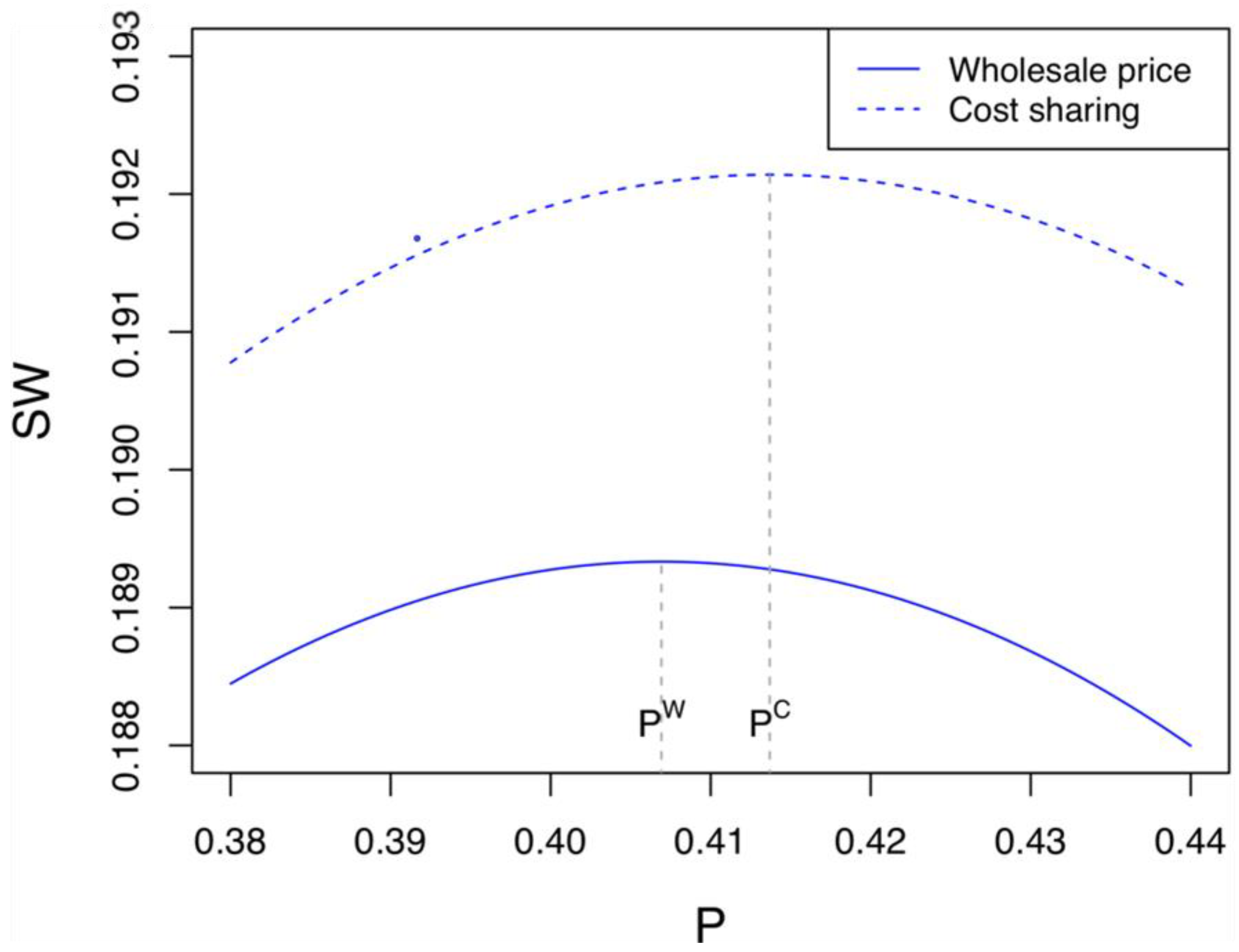
• Is it possible for a government to determine an optimal carbon cap in order to maximize social welfare under both contracts?

The rest of this article is organized as follows. In Section 2, a review of the relevant literature is presented. Section 3 reviews the notations and the assumptions in this article. In Section 4, the main results and various numerical examples are presented. The last section provides a summary and some directions for future research.

2. Literature Review

This section reviews the relevant literature considering three different streams of research on sustainable operations: sustainability innovation, collaboration decisions, and operational management under cap-and-trade regulations.

2.1. Sustainability Innovation in Supply Chains

The topic of sustainable operations is a growing concern for supply chain management [17,18]. Hassini et al. [19] defined sustainable supply chain management as the “management of supply chain operations, resources, information, and funds in order to maximize the supply chain profitability while at the same time minimizing the environmental impacts and maximizing social well-being”. For the purpose of this article, this subsection focuses on sustainability innovations in supply chains.

Product design is a crucial tool for those involved in sustainable development. Krikke et al. [20] suggested a model that integrates product design with a closed-loop supply chain design. By combining costs and environmental impacts into an objective function, they evaluated three potential designs of a refrigerator in different supply chain configurations. Subramanian et al. [21] examined optimal product-design decisions and demonstrated how financial aid could be used as a lever to encourage firms to design environmentally friendly products by considering two key decisions related to product design: performance and remanufacturability. Chen [22] developed a quality-based model that considers the green features of products as a quality attribute and analyzed strategic decision issues related to the development of sustainable products. Shen et al. [23] discussed optimal product line design for green and nongreen products in terms of quality differentiation. They argued that only when the quality difference between green and nongreen products is large enough does designing and selling green products benefit consumers and generate high social welfare. Zhu and He [24] studied green product design in competitive supply chains and derived equilibrium decisions on the greenness degrees of products. Thies et al. [25] conducted a valuable survey of sustainable product designs with extensive bibliographical references

Firms are increasingly paying more attention to sustainable technology innovations in recent years because of stricter regulations and greater consumer concern over corporate social responsibility and environmental protection. The introduction of new product designs and technology/process innovations requires firms to evaluate the complex cost and environmental tradeoffs. Stuart et al. [26] developed a technology selection model for a firm that considers yield, reliability, and environmental impact tradeoffs. They modeled several constraints for environmental effects, including material/energy consumption and technology/process waste generation. Debo et al. [27] solved the issue of joint pricing and production technology selections by manufacturers in the market where new and remanufactured products coexist. They showed that investing in remanufacturing technology is more profitable when there are more environmentally conscious customers in the market. Drake et al. [9] studied the impact of the carbon tax and cap-and-trade regulations on firms’ technology selections and capacity investment decisions. They revealed that a firm’s profits are greater and carbon emissions are lower under governmental cap-and-trade regulations, while production quantities are greater under a carbon tax regulation. Raz et al. [28] considered a newsvendor problem for decisions affecting production quantity and environmentally focused process design efforts. They determined a firm’s sustainable technology innovation efforts at each stage of the product lifecycle.

2.2. Collaboration Decisions in Supply Chain

This work is also related to the literature on supply chain collaboration between manufacturers and their upstream suppliers or downstream retailers. Klassen and Vachon [29] discovered that supply chain collaboration plays a key role in determining both the form and level of environmental technology investments. Zhu et al. [30] and Green et al. [31] also support the view that collaboration between supply chain members on sustainability innovation efforts enhances both environmental and financial performance outcomes and that collaborative innovation is critical for the success of a circular economy initiative.

As pointed out by Ge et al. [32], most studies in this line of research deal with horizontal R&D cooperation in supply chains [33,34,35]. Few papers investigate collaboration among firms with vertical relationships. Talluri et al. [36] considered a manufacturer allocating funds to its suppliers to improve performance and found conditions in which the manufacturer benefits from collaborating with its suppliers. They presented a Markowitz portfolio investment model that can be used to help a manufacturer optimally allocate its available dollars while maintaining expected benefits. Under production cost uncertainty, Kim and Netessine [37] investigated how information asymmetry and procurement contracting strategies affect supply chain members’ incentives to collaborate. According to their results, a manufacturer prefers an expected margin commitment contract if collaboration results in a large reduction in the unit production cost and demand fluctuations are low. Ghosh and Shah [14] explored collaboration issues in a green supply chain and studied the influence of cost-sharing contracts on the key decisions by supply chain members undertaking green initiatives. Two models of cost-sharing contracts were considered—one where a retailer drives a cost-sharing contract and the other where supply chain members negotiate it.

More recently, Ji et al. [38] investigated the collaboration between manufacturers and retailers in online and offline shops and analyzed how a governmental cap-and-trade policy affects supply chain profits and social welfare by adding supply chain members’ efforts to reduce their carbon emissions. Yenipazarli [39] studied the impact of collaboration via supply chain contracts on suppliers’ investments in carbon emission reductions during their manufacturing processes. Further, Dai et al. [15] devised game models to investigate two collaboration mechanisms between supply chain members in relation to green R&D investments: cartelization and cost-sharing contracts. Hong and Lee [16] analyzed two popular contract types, revenue- and cost-sharing contracts, considering the development time uncertainties caused by the R&D capabilities of suppliers. They argued that a contract mechanism to determine the fraction of the revenue or cost that a manufacturer shares with its supplier affects supply chain profits and the expected time required for new product development. Ji et al. [11] derived manufacturer equilibrium production decisions under wholesale pricing and revenue sharing contracts and determined optimal governmental carbon caps. They showed that the equilibrium production quantities increase with a carbon cap, whereas manufacturer profit can decrease with stronger carbon cap regulations. They also found that the overall supply chain profit under a revenue-sharing contract is greater than that under a wholesale price contract. Cachon [40] provided an extensive review of the supply chain literature, focusing on the management of incentive conflicts with contracts, where various contracts in supply chains are identified, and their benefits and drawbacks are illustrated.

2.3. Operations Management under Cap-and-Trade Regulation

Given the increasing severity of global warming, many studies of supply chains with cap-and-trade regulations have been actively conducted over the past few decades. The literature on supply chain management under cap-and-trade regulations includes numerous topics, including pricing, production, inventory, carbon emissions reduction, and carbon cap determination.

Xu et al. [41] studied joint production and the pricing problems of a manufacturer who produces multiple products under cap-and-trade and carbon tax regulations. They presented comparative results on the impacts of the two types of regulation on total carbon emissions, the profits of the firm, and social welfare. Xu et al. [42] extended the work of Xu et al. [41] to study production and pricing issues in a make-to-order (MTO) supply chain with cap-and-trade regulations. Xu et al. [42] analyzed the impact of emission trading prices on the optimal production decisions and the profits of the supply chain members. Bai et al. [43] also considered an MTO supply chain and showed that the profit of a decentralized supply chain can be improved and that carbon emissions can be significantly reduced through supply chain coordination efforts. Yang et al. [44] modeled chain-to-chain competition under cap-and-trade regulations. In their model, each supply chain can either be vertically or horizontally integrated. Yang et al. [44] suggested that a retailer-driven revenue-sharing contract may encourage manufacturers to give up horizontal cooperation, which not only helps all supply chain members achieve a win–win situation but also benefits the environment via a greater reduction in the rate of emissions. Wang et al. [45] examined manufacturing/remanufacturing planning decisions by manufacturers under cap-and-trade regulations. They showed that capital constraints force manufacturers to remanufacture used products at a high level of quality and can considerably reduce carbon emissions. Xu et al. [46] analyzed the equilibrium decisions and coordination mechanisms of a two-echelon supply chain under cap-and-trade regulations and revealed that a two-part tariff contract outperforms a revenue-sharing contract in terms of the profit of a supply chain and the reduction in carbon emissions. Shu et al. [47] dealt with a closed-loop supply chain considering social responsibility and explored the effects of carbon caps and CSR on retailers’ recycling decision behavior. They showed that manufacturers’ CSR has a positive impact on recycling rates and that CSR dramatically leads to a decrease in carbon emissions. From an inventory management perspective, Hua et al. [7] discussed how firms could control carbon emissions as part of their inventory management effort under cap-and-trade regulations. They demonstrated that the carbon cap and emission trading price have a considerable impact on order decisions, carbon emissions, and total costs. Ji et al. [48] analyzed decisions on carbon emissions reductions and inventory replenishment efforts given low-carbon preferences held by consumers. They suggested that a joint carbon tax and cap-and-trade policy work best for emissions reduction and that a government must tighten the carbon cap to realize a clean industry. Shen et al. [49] studied an inventory model for perishable items under a carbon tax policy with collaborative preservation technology investments. They identified optimal decisions on production, delivery, ordering, and investments to maximize the total supply chain profits considering a carbon tax policy. Bai et al. [50] discussed the influence of reducing carbon emissions on the coordination of the supply chain with a vendor-managed inventory system. They showed that a revenue-sharing contract could be introduced to improve profits and reduce carbon emissions in a decentralized supply chain.

Determination of the carbon cap is a crucial decision by a government as part of its work to maximize social welfare. Du et al. [51] considered a supply chain in which an emission-dependent manufacturer and an emission permit supplier interact with each other under cap-and-trade regulations. They determined the optimal allocation of the carbon cap of a manufacturer through consideration of what was termed a fairness distribution in social welfare. Xu et al. [41] found that as the unit environmental damage of a product increases, the government’s optimal carbon cap decreases or remains constant. He et al. [52] studied the optimal production of a self-pricing manufacturer and the optimal carbon cap of a government. They found that the optimal carbon cap and the total carbon emissions initially increase and then decrease as the emissions intensity increases. Ji et al. [11] also argued that if the environmental impact of carbon emissions is low or high, the government should keep the optimal carbon cap unchanged; otherwise, the government may decrease the cap.

3. Research Methodology

As discussed, there are many in-depth studies of sustainable innovations and collaborative decisions in supply chains with carbon emission regulations. The literature review in Section 2 shows that governmental cap-and-trade regulations represent a key factor in the profitability and sustainability of supply chains. However, most studies overlook the relationship between cap-and-trade regulations and manufacturers’ sustainability innovation efforts. Because a significant relationship is found between a carbon cap and decision making in supply chains, it is natural that governmental cap-and-trade regulations affect the sustainability innovation efforts of a supply chain. This article aims to identify the relationship between such a cap and sustainability efforts in a supply chain. Moreover, most studies assumed that carbon trading prices are permanently constant for analytical simplicity, but this article assumes an inverse relationship between a carbon cap and the emission trading price. According to Section 1, the assumption of such an inverse relationship is reasonable and helps supply chain participants gain meaningful managerial insights.

This article provides Stackelberg game models under both wholesale price and cost-sharing contracts and presents the equilibrium decisions made by players of each game. In each game, supply chain participants want to maximize or achieve their goals, and their decisions influence each other. The sequence of each Stackelberg game is detailed in Section 4.

3.1. Notations

This article uses the notations in

Table 1. Notations.

Parameters	Descriptions
$a$	Maximal price of emission credit
$b$	Price sensitivity of carbon cap
$\beta$	Change in production cost as a result of the sustainability effort
$\eta$	Unit environmental damage of carbon emission
$\lambda$	Carbon emission intensity
Decision Variables	Descriptions
$e$	Sustainability effort
$p$	Retail price
$w$	Wholesale price
$P$	Carbon cap
$\delta$	Collaboration level
Functions	Descriptions
$d$	Demand for the product
$M$	Total carbon emission
${\pi }_m$	Manufacturer’s profit
${\pi }_r$	Retailer’s profit
${\pi }_{sc}={\pi }_m+{\pi }_r$	Supply chain profit
$SW$	Social welfare

.

3.2. Assumptions

This article considers a simple supply chain composed of a downstream retailer and an upstream manufacturer that develops a sustainable product. The supply chain distributes only one type of sustainable product. The retailer purchases the manufacturer’s products at the wholesale price $w$. The retailer provides the product to the consumers in the market at a retail price $p$. In the supply chain considered here, the manufacturer makes a sustainability effort $e$, which can boost product demand $d$. This assumption is intuitive because consumers may have higher utility by consuming the sustainable product, meaning that their willingness-to-pay increases, leading to greater demand. Hence, the demand function for the product is formulated as shown below

$$d=1-p+e$$

(1)

As indicated in Equation (1), the potential market base is assumed to be scaled to 1. Note that without a loss of generality, we assume that $e$ has a positive coefficient of one (i.e., effort sensitivity of demand $\gamma =1$). This assumption is justified because the results for an arbitrary $\gamma$ can be obtained by scaling the equilibrium effort $e=\gamma e^{\prime }$.

To capture the decreasing marginal effect of the sustainability efforts, assume that the investment in developing the sustainable product is an increasing and convex function of the efforts. Hence, the effort cost can be expressed as $\theta e^2/2$, where $\theta$ is the cost coefficient of the effort and assume that $\theta =1$ for analytical convenience. In addition, assume that the sustainability effort affects the unit production cost $c=c_0+\beta e$ with the base cost $c_0$ normalized to 0. $\beta$ represents the scenario where the sustainability effort results in an increase in the unit production cost. For example, in the coffee industry, environment-friendly manufacturing processes increase the unit production cost by about 30%. [53]. Additionally, assume that $\beta \in [0,1)$ so that the manufacturer exerts positive sustainability efforts.

Based on an MTO supply chain, this article deals with two types of contracts between the manufacturer and the retailer, specifically a wholesale price contract and a cost-sharing contract. In such a supply chain, the manufacturer and the retailer do not have to focus on the inventory cost or the salvage cost for unsold products. The purpose of this paper is to specify not only the decisions of the supply chain members but also the optimal carbon cap of the government under a cap-and-trade regulation taking into consideration the two types of contracts. Consider the wholesale price contract (cost-sharing contract) as a noncooperative contract (cooperative contract). Under both contracts, the government is assumed to play the role of a Stackelberg game leader. A detailed description of the Stackelberg game under each contract is presented in Section 4. According to the cap-and-trade regulation, the manufacturer is initially given a free quantity of carbon emission credits (also known as carbon emission permits) from a central government. The manufacturer is obligated to hold the credits in an amount larger than or equal to its carbon emissions. The manufacturer can purchase or sell these credits through an outside emissions trading system (ETS). The manufacturer produces the product depending on both the retailer’s order and the allocated cap. In this situation, the government wants to determine the optimal carbon cap which maximizes social welfare.

Let $\lambda$ be the carbon emissions incurred when producing one unit of product. Therefore, the total carbon emissions associated with production is $M=\lambda d$. A similar expression of $M$ can be found in Ji et al. [11] and Gong and Zhou [54]. If the total carbon emission exceeds the given cap (i.e., $M>P$), the manufacturer must purchase the emission credits via the ETS to avoid a large penalty. Otherwise, the manufacturer can sell the excess credits via the ETS to obtain economic incentives. Similar to Hua et al. [7], Benjaafar et al. [8], and Ji et al. [11], assume that the carbon trading price is a linear function of the carbon cap, i.e., $b_0=a-bP\ge 0$ (or equivalently $P\le a/b$), where $a$ is the maximal price of the emission credits and $b$ is the price sensitivity of the cap. The retailer also faces a challenge to lessen the amount of carbon emissions it creates during marketing and selling activities, but the retailer’s carbon emissions are neglected because the amount is relatively small.

4. Analysis and Interpretation of Results

With the notations and assumptions in Section 3, the main results and numerical examples of this article are presented in Propositions and Corollaries. Note that all numerical experiments are carried out based on artificially simulated parameter settings. All proofs in Section 4 are given in Appendix A.

4.1. Equilibrium Analysis with the Given Carbon Cap

This subsection presents the equilibrium decisions of the manufacturer and the retailer with the given carbon cap $P$. Hereafter we utilize the superscript $l\in \{W,C\}$, where $W$ and $C$ represent the wholesale price contract and the cost-sharing contract, respectively.

4.1.1. Wholesale Price Contract

First, consider the wholesale price contract between the manufacturer and the retailer. The profit functions of the manufacturer and the retailer are expressed, respectively, as follows

$${\pi }_m=(w-\beta e)d-\frac{e^2}{2}-(a-bP)(M-P)\mathrm{and}{\pi }_r=(p-w)d,$$

(2)

where ${\pi }_m$ and ${\pi }_r$ denote the profits of the manufacturer and the retailer, respectively. The sequence of the two-stage Stackelberg game under the wholesale price contract is as follows. In the first stage of the game, the manufacturer announces the wholesale price $w$ and the sustainability efforts $e$. After specifying the values of $w$ and $e$, the retailer determines the retail price for the product $p$. Applying backward induction, the equilibrium values of the decision variable and the profit for each player can be obtained in Proposition 1.

Proposition 1.

Given the carbon cap $P$, the equilibrium values in the wholesale price contract game are determined as follows

$$\begin{gathered} w^W=\frac{2-\beta +\lambda (a-bP)}{3-\beta }, p^W=\frac{3+\beta \left(1-\beta +\lambda (a-bP)\right)}{(1+\beta )(3-\beta )}, e^W=\frac{(1-\beta )\left(1-\lambda (a-bP)\right)}{(1+\beta )(3-\beta )},d^W=\frac{1-\lambda (a-bP)}{(1+\beta )(3-\beta )}, \\ {M}^W=\frac{\lambda \left(1-\lambda (a-bP)\right)}{(1+\beta )(3-\beta )}, {\pi }_m^W=\frac{{\left(1-\lambda (a-bP)\right)}^2}{2(1+\beta )(3-\beta )}+P(a-bP), and {\pi }_r^W={\left(\frac{1-\lambda (a-bP)}{(1+\beta )(3-\beta )}\right)}^2. \end{gathered}$$

(3)

When the government initially sets the carbon cap to zero, the inequality $a\lambda <1$ should be assumed to avoid negative demand for the product. From Proposition 1, Corollaries 1–3 can be derived as shown below.

Corollary 1.

Under the wholesale price contract, the equilibrium decisions have the following relationships:

$$\frac{\partial w^W}{\partial P}<0, \frac{\partial p^W}{\partial P}<0, \frac{\partial e^W}{\partial P}>0, \frac{\partial d^W}{\partial P}>0, and \frac{\partial M^W}{\partial P}>0.$$

(4)

Corollary 1 presents the important fact that the equilibrium decision of each supply chain member depends on the carbon cap. The equilibrium wholesale price decreases with the carbon cap, which encourages the retailer to decrease its retail price. As a result, the demand for the product inevitably increases. This occurs because as the allocated carbon cap increases, the carbon trading price decreases, which leads to a higher marginal profit per unit of the product. Another important fact is that the manufacturer’s sustainability effort increases as the carbon cap increases. The manufacturer can obtain higher profits as it produces more products. Therefore, the manufacturer may try to increase the demand for the product, which requires a greater sustainability effort. As the carbon cap increases, sustainability efforts increase, and the manufacturer can thus obtain higher profits. As the cap increases, the production quantity also increases, resulting in more carbon emissions.

Corollary 2.

Under the wholesale price contract, the equilibrium profits have the following relationships:

$$\frac{\partial {\pi }_r^W}{\partial P}>0and\frac{\partial {\pi }_m^W}{\partial P}=\{\begin{array}{l}>0,if0<b<K_{1}and0<P<K_2,\\ >0,ifb>K_1,\\ <0,if0<b<K_{1}andP>K_2,\end{array}$$

(5)

where$K_1=\frac{2(1+\beta )(3-\beta )}{{\lambda }^2}$and$K_2=\frac{a(1+\beta )(3-\beta )+b\lambda (1-a\lambda )}{b\left(2(1+\beta )(3-\beta )-b{\lambda }^2\right)}$.

Corollary 2 expresses the relationship between the equilibrium profit and the carbon cap. As indicated in Equation (5), the retailer’s equilibrium profit increases with respect to the cap. This conclusion is rather intuitive because the higher the carbon cap, the higher the retailer’s marginal profit and the higher the demand for the product and the retailer’s profit will increase as well. When the price sensitivity of the carbon cap $b$ is lower than the threshold $K_1$, the trend of the manufacturer’s profit with respect to the carbon cap differs based on the range of the cap. That is, if the cap is under the threshold $K_2$, the manufacturer’s profit increases along with the cap. Otherwise, the manufacturer’s profit decreases. This means that the manufacturer’s profit reaches its maximum when the government sets the carbon cap to $K_2$. In contrast, when $b$ exceeds the threshold $K_1$, the manufacturer’s profit always increases with the cap. Figure 1 illustrates the relationship between the carbon cap and the manufacturer’s profit with the following parameter settings: $\lambda =0.8$, $\beta =0.05$, $a=1$, $K_1=9.68$ (a) $b=0.5<K_1$, and (b) $b=10>K_1$, which confirms that when $0<b<K_1$, the maximal manufacturer’s profit is obtained at $K_2=1.0817$, and also confirms that when $b>K_1$, the manufacturer’s profit increases with the cap. In previous studies, such as Xu et al. [41], Gong and Zhou [54], Zhang and Xu [55], Du et al. [56], Xu et al. [57], and Zhang et al. [58], it is argued that the carbon cap always has a positive impact on the manufacturer’s profit. However, our result shows that the manufacturer’s profit is either positively or negatively affected by the carbon cap; thus, determining the appropriate carbon cap is crucial for the manufacturer.

Corollary 3.

Under the wholesale price contract, the manufacturer purchases$M^W-P$emission credits if either Condition 1 or 2 is met. Meanwhile, the manufacturer sells$P-M^W$emission credits if Condition 3 is met.

 (i)

Condition 1:$0<b<K_3 and 0<P<K_4$,

 (ii)

Condition 2:$b>K_3$,

 (iii)

Condition 3:$0<b<K_3 and P>K_4$,

where$K_3=\frac{(1+\beta )(3-\beta )}{{\lambda }^2}$and$K_4=\frac{\lambda (1-a\lambda )}{(1+\beta )(3-\beta )-b{\lambda }^2}$.

Corollary 3 shows the manufacturer’s equilibrium behavior for purchasing/selling emission credits. When the price sensitivity of the carbon cap $b$ is under the threshold $K_3$, the manufacturer’s purchasing/selling behavior differs according to the range of the carbon cap. If the cap is lower than the threshold $K_4$, the manufacturer must purchase additional emission credits to avoid the penalty and enhance the cap level. Otherwise, the manufacturer is willing to sell excess emission credits to achieve a financial incentive. In contrast, when $b$ exceeds the threshold $K_3$, the manufacturer always purchases the emission credits. In summary, there is a threshold for purchasing and selling the emission credits because of the linearly inverse relationship between the carbon cap and the emission trading price. Figure 2 depicts the manufacturer’s decision on purchasing/selling the emission credits with the following parameter settings: $\lambda =0.5$, $\beta =0.05$, $a=0.4$, $K_3=12.39$, $K_4=0.1469$, (a) $b=1.5<K_3$, and (b) $b=13>K_3$. Figure 2a shows that the manufacturer purchases (sells) $M^W-P$ ($P-M^W$) emission credits if $P<K_4$ ($P>K_4$). If $P=K_4$, the manufacturer neither purchases nor sells the emission credits because $M^W=P$. Meanwhile, as shown in Figure 2b, the manufacturer always purchases $M^W-P$ emission credits if $b>K_3$.

4.1.2. Cost-Sharing Contract

Next, consider the collaboration model. Under a cost-sharing contract between supply chain members, the retailer shares $\delta$ fraction of the manufacturer’s cost related to the production and sustainability innovation efforts. The profit functions of the manufacturer and the retailer are then expressed, respectively, as shown below.

$${\pi }_m=\left(w-(1-\delta )\beta e\right)d-\frac{(1-\delta )e^2}{2}-(a-bP)(M-P)and{\pi }_r=(p-w-\delta \beta e)d-\frac{\delta e^2}{2}.$$

(6)

Under the cost-sharing contract, the sequence of the three-stage Stackelberg game is as follows. In the first stage, the retailer determines the collaboration level $\delta$ that maximizes its profit. In the second stage, the manufacturer announces the wholesale price $w$ and the sustainability effort $e$. After specifying the values of $w$ and $e$, the retailer determines the retail price for the product $p$ in the last stage. Applying backward induction, the equilibrium values of the decision variable and the profit for each player are obtained in Proposition 2.

Proposition 2.

Given the carbon cap$P$, the equilibrium values in the cost-sharing contract game are determined as follows:

$$\begin{gathered} {\delta }^C=\frac{{(1-\beta )}^2}{8}, w^C=\frac{(1+\beta )(2-\beta )(7+2\beta -{\beta }^2)+\lambda (a-bP)(3-\beta )(2+5\beta +{\beta }^3)}{4(5+6\beta -3{\beta }^2)}, \\ {p}^C=\frac{21+14\beta -11{\beta }^2-\lambda (a-bP)(1-10\beta +{\beta }^2)}{4(5+6\beta -3{\beta }^2)}, e^C=\frac{2(1-\beta )\left(1-\lambda (a-bP)\right)}{5+6\beta -3{\beta }^2}, \\ {d}^C=\frac{(7+2\beta -{\beta }^2)\left(1-\lambda (a-bP)\right)}{4(5+6\beta -3{\beta }^2)}, M^C=\frac{\lambda (7+2\beta -{\beta }^2)\left(1-\lambda (a-bP)\right)}{4(5+6\beta -3{\beta }^2)}, \\ {\pi }_m^C=\frac{(7+2\beta -{\beta }^2){\left(1-\lambda (a-bP)\right)}^2}{8(5+6\beta -3{\beta }^2)}+P(a-bP), and {\pi }_r^C=\frac{(9-2\beta +{\beta }^2){\left(1-\lambda (a-bP)\right)}^2}{16(5+6\beta -3{\beta }^2)}. \end{gathered}$$

(7)

Under the cost-sharing contract, we assume that $a\lambda <1$ to avoid the negative demand for the product. Note that the equilibrium retailer’s collaboration level must be lower than 0.125 because ${\delta }^C$ is a decreasing function when $\beta \in (0,1)$. From Proposition 2, Corollaries 4–6 are derived as shown below.

Corollary 4.

Under the cost-sharing contract, the equilibrium decisions have the following relationships:

$$\frac{\partial w^C}{\partial P}<0, \frac{\partial e^C}{\partial P}>0, \frac{\partial d^C}{\partial P}>0,\frac{\partial M^C}{\partial P}>0, and \frac{\partial p^C}{\partial P}=\{\begin{array}{l}>0, if 0<\beta <5-2\sqrt{6},\\ <0, if 5-2\sqrt{6}<\beta <1.\end{array}$$

(8)

Under the cost-sharing contract, if $0<\beta <5-2\sqrt{6}$ ($5-2\sqrt{6}<\beta <1$), the retail price increases (decreases) with respect to the carbon cap. Regarding the wholesale price, the sustainability effort, and the demand for the product, relationships similar to Corollary 1 are found. Accordingly, further statements are omitted.

Corollary 5.

Under the cost-sharing contract, the equilibrium profits have the following relationships:

$$\frac{\partial {\pi }_r^C}{\partial P}>0and\frac{\partial {\pi }_m^C}{\partial P}=\{\begin{array}{l}>0, if 0<b<K_5 and 0<P<K_6,\\ >0, if b>K_5,\\ <0, if 0<b<K_5 and P>K_6,\end{array}$$

(9)

where$K_5=\frac{8(5+6\beta -3{\beta }^2)}{{\lambda }^2(7+2\beta -{\beta }^2)}$and$K_6=\frac{4a(5+6\beta -3{\beta }^2)+b\lambda (1-a\lambda )(7+2\beta -{\beta }^2)}{b\left(8(5+6\beta -3{\beta }^2)-b{\lambda }^2(7+2\beta -{\beta }^2)\right)}$.

Corollary 5 shows results similar to those of Corollary 2. Even under the cost-sharing contract, the retailer’s profit increases as the carbon cap increases. When the price sensitivity of the carbon cap $b$ is under the threshold $K_5$, the trend of the manufacturer’s profit differs according to the range of the cap. That is, if the cap is under (exceeds) threshold $K_6$, the manufacturer’s profit increases (decreases) along with the cap. Hence, the manufacturer obtains its maximal profit at $P=K_6$. On the other hand, when $b$ exceeds the threshold $K_5$, the manufacturer’s profit always increases. Comparing the critical cap shown in Corollaries 2 and 5, the following relation is found that

$$K_6-K_2=\frac{\lambda (2-a\lambda )(1-{\beta }^4)}{\left(2(3-\beta )(1+\beta )-b{\lambda }^2\right)\left(8(5+6\beta -3{\beta }^2)-b{\lambda }^2(7+2\beta -{\beta }^2)\right)}>0,$$

(10)

which means that by adopting the cost-sharing contract, the manufacturer maintains its profit growth with a relatively higher carbon cap. This argument is depicted in Figure 3 with the following parameter settings: $\lambda =0.8$, $\beta =0.05$, $a=1$, $b=0.5$, $K_2=1.0817$, and $K_6=1.085$.

Corollary 6.

Under the cost-sharing contract, the manufacturer purchases$M^C-P$emission credits if either Condition 4 or 5 is met. Meanwhile, the manufacturer sells$P-M^C$emission credits if Condition 6 is met.

 (i)

Condition 4:$0<b<K_7 and 0<P<K_8$,

 (ii)

Condition 5:$b>K_7$,

 (iii)

Condition 6:$0<b<K_7 and P>K_8$,

where$K_7=\frac{4(5+6\beta -3{\beta }^2)}{{\lambda }^2(7+2\beta -{\beta }^2)}$and$K_8=\frac{\lambda (1-a\lambda )(7+2\beta -{\beta }^2)}{4(5+6\beta -3{\beta }^2)-b{\lambda }^2(7+2\beta -{\beta }^2)}$.

Corollary 6 shows the manufacturer’s equilibrium decision with regard to purchasing/selling the emission credits under the cost-sharing contract. Corollary 6 is similar to Corollary 3; thus, redundant statements are omitted here. Comparing the critical cap shown in Corollaries 3 and 6, the following relation is found that

$$K_8-K_4=\frac{\lambda (1-a\lambda )(1-{\beta }^4)}{\left((3-\beta )(1+\beta )-b{\lambda }^2\right)\left(4(5+6\beta -3{\beta }^2)-b{\lambda }^2(7+2\beta -{\beta }^2)\right)}>0,$$

(11)

which means that the threshold of purchasing/selling the emission credits with the cost-sharing contract is higher than that under the wholesale price contract. Figure 4 shows the difference in the manufacturer’s carbon trading decision between the wholesale price contract and the cost-sharing contract with the following parameter settings: $\lambda =0.5$, $\beta =0.05$, $a=0.4$, $b=1.5$, $K_4=0.1469$, and $K_8=0.1534$. Figure 4 confirms the following: (i) when $P<K_4$, the manufacturer must purchase additional emission credits under both contracts; (ii) when $P>K_8$, the manufacturer can sell excess emission credits under both contracts; and (iii) when $K_4<P<K_8$, the manufacturer purchases emission credits under the cost-sharing contract, whereas it sells them under the wholesale price contract.

4.1.3. Comparison

One may be curious about the differences in the equilibrium values between two contracts. This subsection conducts a comparative analysis by comparing Propositions 1 and 2. The result is as follows.

Corollary 7.

The following relation is found that

$$e^W<e^C, d^W<d^C, w^W<w^C, p^W<p^C, M^W<M^C, {\pi }_m^W<{\pi }_m^C, {\pi }_r^W<{\pi }_r^C, and {\pi }_{sc}^W<{\pi }_{sc}^C.$$

(12)

Corollary 7 shows that a cost-sharing contract outperforms a wholesale price contract in terms of the profitability and sustainability of a supply chain. It must be first noted that the sustainability effort under the cost-sharing contract is greater than that under the wholesale price contract. Cost sharing with the retailer can help the manufacturer reduce the burden of product development and reduce production costs, ultimately leading to greater sustainability efforts. This makes it possible for the product to become more sustainable, which increases consumer utility as well as the demand for the product. Let $m^W$ and $m^C$ denote the marginal cost under the wholesale price and cost-sharing contracts, respectively. Following Equations (2) and (6), the relation $m^W=\beta e^W<(1-{\delta }^C)\beta e^C=m^C$ is obtained. That is, the higher marginal cost under the cost-sharing contract forces the manufacturer to raise the wholesale price, which results in an increase in the retail price. Corollary 7 also confirms that the profit of each supply chain member as well as the supply chain profit will increase if the retailer adopts a cost-sharing contract. Under the cost-sharing contract, the demand and prices increase at the same time, resulting in a natural increase in the profit of each supply chain member and leading to an increase in the overall supply chain profits. Finally, more carbon emissions are inevitable owing to the increased production of the product under the cost-sharing contract.

4.2. Government’s Optimal Decision on Carbon Cap

Thus far, this article has regarded the carbon cap $P$ as an exogenous parameter initially set by the government. However, henceforth, we consider $P$ as an endogenous decision variable. In reality, the government may have a goal when implementing cap-and-trade regulations. Assume that the following possible objective is considered by the government: the government wants to maximize social welfare. By determining the optimal carbon cap, the government will achieve this objective.

Once again, this section analyzes the government’s optimal decisions regarding the carbon cap under both contracts. To do this, we initially formulate the revenue and cost terms separately. We then integrate them to derive the objective function of the government problem. Social welfare $SW$ is a function of the cap and takes the form of

$$SW(P)={\displaystyle {\int }_p^{p_{\max }}(1-p+e)dp}+{\pi }_{sc}-\eta M,$$

(13)

where $p_{\max }$ is the maximum price of the product. The first term ${\displaystyle {\int }_p^{p_{\max }}(1-p+e)dp}$ represents the value of the consumer surplus, which, in economics, is defined as the gap between the maximum price consumers are willing to pay and the actual price they pay. From simple algebra, it is obtained that ${\displaystyle {\int }_p^{p_{\max }}(1-p+e)dp}=d^2/2$. The second term is the supply chain profit, which is defined as the sum of the manufacturer’s and retailer’s profits. The government wants to minimize environmental degradation as the manufacturer produces the product. Let $\eta$ be the unit environmental impact of the product. The coefficient $\eta$ measures the degree of environmental damage due to the manufacturer’s production process and the associated pollutants in monetary terms. Thus, the total environmental damage costs caused by production are expressed as $\eta M$. It is important to note that the carbon trading cost (revenue) is not included in the social welfare function in Equation (13) because it is a transaction between the manufacturer and the government.

Assume that the government is an overall game leader under both a wholesale price contract and a cost-sharing contract. Let $P^l$ denote the equilibrium carbon cap. Under each contract, $P^l$ is obtained by solving the following maximization problem:

$$P^l=\underset{0\le P\le a/b}{\arg \max }S{W}^l(P), for l\in \{W,C\}.$$

(14)

The main results of this subsection are presented in Propositions 3 and 4.

Proposition 3.

Under the wholesale price contract, the government’s optimal decision on the carbon cap is given by:

 (i)

If$b<K_9$,$P^W=\frac{a\left({(1+\beta )}^2{(3-\beta )}^2-b{\lambda }^2(6+2\beta -{\beta }^2)\right)+b\lambda \left(6-3\eta \lambda +\beta (2-\beta )(1-\eta \lambda )\right)}{b\left(2{(1+\beta )}^2{(3-\beta )}^2-b{\lambda }^2(6+2\beta -{\beta }^2)\right)}$,

 (ii)

If$b=K_9$and$\eta >K_{10}$,$P^W=0$,

 (iii)

If$b=K_9$and$\eta <K_{10}$,$P^W=\frac{a}{b}$,

 (iv)

If$b>K_9$,$P^W=\frac{a}{b}$,

where$K_9=\frac{2{(1+\beta )}^2{(3-\beta )}^2}{{\lambda }^2(6+2\beta -{\beta }^2)}$and$K_{10}=\frac{(6+2\beta -{\beta }^2)(2-a\lambda )}{2\lambda (1+\beta )(3-\beta )}$.

Proposition 3 shows that the government’s optimal decision about the carbon cap differs based on the price sensitivity of the cap $b$ and the unit environmental impact cost $\eta$. If $b<K_9$, the social welfare function is strictly concave with respect to the cap; therefore, solving the first-order condition determines the global maximizer of the government’s problem in Equation (14). If $b=K_9$ and $\eta >K_{10}$ ($\eta <K_{10}$), social welfare is a linearly decreasing (increasing) function of the carbon cap; thus, the optimal carbon cap equals zero ($a/b$). Lastly, social welfare is a convex and increasing function of the cap if $b>K_9$. Accordingly, the optimal carbon cap equals $a/b$. Figure 5 depicts Proposition 3 with the following parameter settings: $\lambda =0.8$, $\beta =0.1$, $a=1$, $K_9=5.1374$, and $K_{10}=1.4553$. In Figure 5a, the set $b=2<K_9$, and the social welfare is maximized at $P^C=0.3248$. Figure 5b–d correspond to Proposition 3(ii), 3(iii) and 3(iv), respectively.

Proposition 4.

Under the cost-sharing contract, the government’s optimal decision on the carbon cap is given by

 (i)

If$b<K_{11}$,$P^C=\frac{\begin{array}{l}a\left(16{(5+6\beta -3{\beta }^2)}^2-b{\lambda }^2(279+324\beta -134{\beta }^2-28{\beta }^3+7{\beta }^4)\right)\\ +b\lambda \left(279+324\beta -134{\beta }^2-28{\beta }^3+7{\beta }^4-4\eta \lambda (5+6\beta -3{\beta }^2)(7+2\beta -{\beta }^2)\right)\end{array}}{b\left(32{(5+6\beta -3{\beta }^2)}^2-b{\lambda }^2(279+324\beta -134{\beta }^2-28{\beta }^3+7{\beta }^4)\right)}$,

 (ii)

If$b=K_{11}$and$\eta >K_{12}$,$P^C=0$,

 (iii)

If$b=K_{11}$and$\eta <K_{12}$,$P^C=\frac{a}{b}$,

 (iv)

If$b>K_{11}$,$P^C=\frac{a}{b}$,

where$K_{11}=\frac{32{(5+6\beta -3{\beta }^2)}^2}{{\lambda }^2(279+324\beta -134{\beta }^2-28{\beta }^3+7{\beta }^4)}$and$K_{12}=\frac{4(5+6\beta -3{\beta }^2)(2-a\lambda )}{b{\lambda }^3(7+2\beta -{\beta }^2)}$.

Proposition 4 presents the government’s optimal decision regarding the carbon cap under the cost-sharing contract. Because Proposition 4 is similar to Proposition 3, we skip any redundant explanations. Following Propositions 3 and 4, Corollaries 8 and 9 are obtained as follows:

Corollary 8.

Assuming b < min{K₉, K₁₁}, it is found that

$$\frac{\partial P^l}{\partial \eta }<0, \mathit{for} l\in \{W,C\}.$$

(15)

Corollary 8 confirms that the carbon cap decreases as the unit environmental impact cost $\eta$ increases. As indicated in Equation (13), $\eta$ has a negative influence on social welfare. When $\eta$ increases, the total environmental damage cost also increases; thus, the government wants to reduce the environmental damage by reducing the production quantity of the product. In our model, the only way for the government to reduce the manufacturer’s production quantity is to lower the carbon cap. Note that from Corollaries 1 and 4, the demand for the product decreases as the carbon cap decreases.

Corollary 9.

Assumingb < $\min \{K_9,K_{11}\}$, it is found that

$$P^W-P^C=\{\begin{array}{l}\le 0, if \eta \le K_{13}=\frac{(2-a\lambda )(111+148\beta -46{\beta }^2-28{\beta }^3+7{\beta }^4)}{8\lambda (1+\beta )(3-\beta )(5+6\beta -3{\beta }^2)-b{\lambda }^3(3+10\beta -5{\beta }^2)},\\ >0, otherwise.\end{array}$$

(16)

Corollary 9 shows a comparison of the carbon caps under each contract. If $\eta$ is low, the government sets a higher carbon cap under the cost-sharing contract. By setting a higher carbon cap when $\eta$ is relatively low, the government wants to maintain the cooperation between the manufacturer and the retailer for greater supply chain profit and greater consumer surplus. On the other hand, if $\eta$ is high, the government sets a higher carbon cap under the wholesale price contract. By doing so, the government encourages the manufacturer to increase its sustainable innovation efforts, which boosts the demand for the product. The increased demand raises consumer surplus as well as the supply chain profit, which compensates for the total environmental impact cost. Figure 6 shows a comparison between the optimal carbon caps under each type of contract with the following parameter settings: $\lambda =0.8$, $\beta =0.1$, $a=1$, $b=2$, $\eta =0.5$, $K_{13}=1.3711$, $P^W=0.4069$, and $P^C=0.4137$. As illustrated in Figure 6, the optimal carbon cap under the cost-sharing contract is greater than that under the wholesale price contract when $\eta$ is under the threshold $K_{13}$.

5. Conclusions

This article discussed equilibrium decisions about pricing and sustainability efforts in a supply chain under wholesale price and cost-sharing contracts. The major findings of this article are summarized below:

• Under wholesale price and cost-sharing contracts, the carbon cap has a positive impact on the manufacturer’s sustainability efforts, which leads to an increase in the demand for the product. Because of the increased demand, the wholesale and retail prices fall at the same time;
• Under both contracts, the retailer’s profit increases with respect to the carbon cap. Therefore, the retailer would like the government to set a higher carbon cap. However, the manufacturer’s profit does not increase consistently with a higher carbon cap. This implies that proper cap setting has a significant impact on the manufacturers’ profit;
• The cost-sharing contract outperforms the wholesale price contract in terms of product demand, prices, and the profitability of supply chain members. This fact reveals that the cost-sharing contract is a win–win strategy for both the manufacturer and the retailer. Under the cost-sharing contract, the profitability of the supply chain can improve, which has a positive impact on the sustainability of the supply chain. Because of the increasing manufacturers’ profits, they can invest in more sustainable product development and manufacturing processes. This makes the supply chain more sustainable. Therefore, policy makers must provide subsidies and legal systems related to supply chain cooperation to provide a business environment in which supply chain members can collaborate more easily and efficiently;
• When the government wants to determine the carbon cap under both contracts, there is an optimal cap that maximizes social welfare. This optimal carbon cap decreases when the environmental damage caused by the production of the product increases. It is also found that when this type of environmental damage is relatively low, the government sets a higher cap under the cost-sharing contract so that the supply chain members maintain their cooperation.

This article provides several recommendations for firms that undertake sustainability efforts and face carbon emission constraints. However, there are also limitations that can be expanded upon and improved in future research: (1) Newsvendor model: the assumption of uncertain demand for the product is more complex but more realistic; (2) retailer’s sustainability effort: an extended model can assume that the retailer can participate in sustainability activities, such as green retailing and green marketing; (3) other contracts: a comparative analysis of other supply chain cooperation contracts will provide more meaningful insights; and (4) multiple participants: in reality, multiple manufacturers and retailers either collaborate or compete in various supply chains. It would be worthwhile to analyze a supply chain with more complex but realistic conditions.

References

1. One day We’ll Disappear: Tuvalu’s Sinking Islands. Available online: http://www.theguardian.com/global-development/2019/may/16/one-day-disappear-tuvalu-sinking-islands-rising-seas-climate-change (accessed on 2 February 2022).
2. Disappearing Island Nations are the Sinking Reality of Climate Change. Available online: http://qrius.com/disappearing-island-nations-are-the-sinking-reality-of-climate-change/ (accessed on 4 February 2022).
3. It’s Official: Sea Level Rise Could Soon Displace Up to 187 Million People. Available online: http://www.sciencealert.com/sea-level-rise-could-displace-187-million-climate-refugees (accessed on 4 February 2022).
4. Climate Migrants Might Reach One Billion by 2050. Available online: http://reliefweb.int/report/world/climate-migrants-might-reach-one-billion-2050 (accessed on 4 February 2022).
5. Mechanisms under the Kyoto Protocol. Available online: http://unfccc.int/process/the-kyoto-protocol/mechanisms (accessed on 5 February 2022).
6. Velazquez-Cazares, M.G.; Leon-Castro, E.; Blanco-Mesa, F.; Alvarado-Altamirano, S. The ordered weighted average corporate social responsibility. Kybernetes 2021, 50, 203–220. [Google Scholar] [CrossRef]
7. Hua, G.; Cheng, T.C.E.; Wang, S. Managing carbon footprints in inventory management. Int. J. Prod. Econ. 2011, 132, 178–185. [Google Scholar] [CrossRef]
8. Benjaafar, S.; Li, Y.; Daskin, M. Carbon Footprint and the Management of Supply Chains: Insights from Simple Models. IEEE Trans. Autom. Sci. Eng. 2013, 10, 99–116. [Google Scholar] [CrossRef]
9. Drake, D.F.; Kleindorfer, P.R.; van Wassenhove, L.N. Technology choice and capacity portfolios under emissions regulation. Prod. Oper. Manag. 2016, 25, 1006–1025. [Google Scholar] [CrossRef]
10. Benz, E.; Trück, S. Modeling the Price Dynamics of CO2 Emission Allowances. Energy Econ. 2009, 31, 4–15. [Google Scholar] [CrossRef]
11. Ji, T.; Xu, X.; Yan, X.; Yu, Y. The production decisions and cap setting with wholesale price and revenue sharing contracts under cap-and-trade regulation. Int. J. Prod. Res. 2020, 58, 128–147. [Google Scholar] [CrossRef]
12. Chao, G.H.; Iravani, S.M.; Savaskan, R.C. Quality improvement incentives and product recall cost sharing contracts. Manag. Sci. 2009, 55, 1122–1138. [Google Scholar] [CrossRef] [Green Version]
13. Leng, M.; Parlar, M. Game-theoretic analyses of decentralized assembly supply chains: Non-cooperative equilibria vs. coordination with cost-sharing contracts. Eur. J. Oper. Res. 2010, 204, 96–104. [Google Scholar] [CrossRef]
14. Ghosh, D.; Shah, J. Supply chain analysis under green sensitive consumer demand and cost sharing contract. Int. J. Prod. Econ. 2015, 164, 319–329. [Google Scholar] [CrossRef]
15. Dai, R.; Zhang, J.; Tang, W. Cartelization or Cost-sharing? Comparison of cooperation modes in a green supply chain. J. Clean. Prod. 2017, 156, 159–173. [Google Scholar] [CrossRef]
16. Hong, J.; Lee, P. Supply chain contracts under new product development uncertainty. Sustainability 2019, 11, 6858. [Google Scholar] [CrossRef] [Green Version]
17. Drake, D.F.; Spinler, S. Sustainable operations management: An enduring stream or a passing fancy. Manuf. Serv. Oper. Manag. 2013, 15, 689–700. [Google Scholar] [CrossRef] [Green Version]
18. Beltagui, A.; Kunz, N.; Gold, S. The role of 3D printing and open design on adoption of socially sustainable supply chain innovation. Int. J. Prod. Econ. 2020, 221, 107462. [Google Scholar] [CrossRef]
19. Hassini, E.; Surti, C.; Searcy, C. A literature review and a case study of sustainable supply chains with a focus on metrics. Int. J. Prod. Econ. 2012, 140, 69–82. [Google Scholar] [CrossRef]
20. Krikke, H.; Bloemhof-Ruwaard, J.; van Wassenhove, L.N. Concurrent product and closed-loop supply chain design with an application to refrigerator. Int. J. Prod. Res. 2003, 42, 3689–3719. [Google Scholar] [CrossRef]
21. Subramanian, R.; Gupta, S.; Talbot, B. Product design and supply coordination under extended producer responsibility. Prod. Oper. Manag. 2009, 18, 259–277. [Google Scholar] [CrossRef]
22. Chen, C. Design for the environment: A quality-based model for green product development. Manag. Sci. 2001, 47, 250–263. [Google Scholar] [CrossRef]
23. Shen, B.; Cao, Y.; Xu, X. Product line design and quality differentiation for green and non-green products in a supply chain. Int. J. Oper. Res. 2020, 58, 148–164. [Google Scholar] [CrossRef]
24. Zhu, W.; He, Y. Green product design in supply chains under competition. Eur. J. Oper. Res. 2017, 258, 165–180. [Google Scholar] [CrossRef]
25. Thies, C.; Kieckhäfer, K.; Spengler, T.S.; Sodhi, M.S. Operations Research for Sustainability Assessment of Products: A Review. Eur. J. Oper. Res. 2019, 274, 1–21. [Google Scholar] [CrossRef]
26. Stuart, J.A.; Ammons, J.C.; Turbini, L.J. A product and process selection model with multidisciplinary environmental considerations. Oper. Res. 1999, 47, 221–234. [Google Scholar] [CrossRef]
27. Debo, L.G.; Toktay, L.B.; van Wassenhove, L.N. Market segmentation and product technology selection for remanufacturing. Manag. Sci. 2005, 47, 881–893. [Google Scholar]
28. Raz, G.; Druehl, C.T.; Blass, V. Design for the environment: Life-cycle approach using a newsvendor model. Prod. Oper. Manag. 2013, 22, 940–957. [Google Scholar] [CrossRef]
29. Klassen, R.; Vachon, S. Collaboration and evaluation in the supply chain: The impact on plant-level environmental investment. Prod. Oper. Manag. 2003, 12, 336–352. [Google Scholar] [CrossRef]
30. Zhu, Q.; Geng, Y.; Lai, K. Circular economy practices among Chinese manufacturers varying in environmental-oriented supply chain cooperation and the performance implications. J. Environ. Manag. 2010, 91, 1324–1331. [Google Scholar] [CrossRef]
31. Green, K.W., Jr.; Zelbst, P.J.; Bhadauria, V.S.; Meacham, J. Do environmental collaboration and monitoring enhance organizational performance? Ind. Manag. Data Syst. 2012, 112, 186–205. [Google Scholar] [CrossRef]
32. Ge, Z.; Hu, Q.; Xia, Y. Firms’ R&D cooperation behavior in a supply chain. Prod. Oper. Manag. 2014, 23, 599–609. [Google Scholar]
33. Bhaskaran, S.R.; Krishnan, V. Effort, revenue, and cost sharing mechanisms for collaborative new product development. Manag. Sci. 2009, 55, 1152–1169. [Google Scholar] [CrossRef] [Green Version]
34. Ge, Z.; Hu, Q. Collaboration in R&D activities: Firm-specific decisions. Eur. J. Oper. Res. 2008, 185, 864–883. [Google Scholar]
35. Veugelers, R. Collaboration in R&D: An assessment of theoretical and empirical findings. Economist 1998, 146, 419–443. [Google Scholar]
36. Talluri, S.; Narasimhan, R.; Chung, W. Manufacturer cooperation in supplier development under risk. Eur. J. Oper. Res. 2010, 207, 165–173. [Google Scholar] [CrossRef]
37. Kim, S.-H.; Netessine, S. Collaborative cost reduction and component procurement under information asymmetry. Manag. Sci. 2013, 59, 189–206. [Google Scholar] [CrossRef] [Green Version]
38. Ji, J.; Zhang, Z.; Yang, L. Comparisons of initial carbon allowance allocation rules in an O2O retail supply chain with the cap-and-trade regulation. Int. J. Prod. Econ. 2017, 187, 68–84. [Google Scholar] [CrossRef]
39. Yenipazarli, A. To collaborate or not to collaborate: Prompting upstream eco-efficient innovation in a supply chain. Eur. J. Oper. Res. 2017, 260, 571–587. [Google Scholar] [CrossRef]
40. Cachon, G.P. Handbooks in Operations Research and Management Science: Supply Chain Management: Design, Coordination and Operations; Elsevier: Amsterdam, The Netherlands, 2003; pp. 227–339. [Google Scholar]
41. Xu, X.; Xu, X.; He, P. Joint production and pricing decisions for multiple products with cap-and-trade and carbon tax regulations. J. Clean. Prod. 2016, 112, 4093–4106. [Google Scholar] [CrossRef]
42. Xu, X.; Zhang, W.; He, P.; Xu, X. Production and pricing problems in make-to-order supply chain with cap-and-trade regulation. Omega 2017, 66, 248–257. [Google Scholar] [CrossRef]
43. Bai, Q.; Xu, J.; Zhang, Y. Emission reduction decision and coordination of a make-to-order supply chain with two products under cap-and-trade regulation. Comput. Ind. Eng. 2018, 119, 131–145. [Google Scholar] [CrossRef]
44. Yang, L.; Zhang, Q.; Ji, J. Pricing and carbon emission reduction decisions in supply chains with vertical and horizontal cooperation. Int. J. Prod. Econ. 2017, 191, 286–297. [Google Scholar] [CrossRef]
45. Wang, Y.; Chen, W.; Liu, B. Manufacturing/remanufacturing decisions for a capital-constrained manufacturer considering carbon emission cap and trade. J. Clean. Prod. 2017, 140, 1118–1128. [Google Scholar] [CrossRef]
46. Xu, J.; Chen, Y.; Bai, Q. A two-echelon sustainable supply chain coordination under cap-and-trade regulation. J. Clean. Prod. 2016, 112, 42–56. [Google Scholar] [CrossRef]
47. Shu, T.; Liu, Q.; Chen, S.; Wang, S.; Lai, K.K. Pricing decisions of CSR closed-loop supply chains with carbon emission constraints. Sustainability 2018, 10, 4430. [Google Scholar] [CrossRef] [Green Version]
48. Ji, S.; Zhao, D.; Peng, X. Joint decisions on emission reduction and inventory replenishment with overconfidence and low-carbon preference. Sustainability 2018, 10, 1119. [Google Scholar] [CrossRef] [Green Version]
49. Shen, Y.; Shen, K.; Yang, C. A production inventory model for deteriorating items with collaborative preservation technology investment under carbon tax. Sustainability 2019, 11, 5027. [Google Scholar] [CrossRef] [Green Version]
50. Bai, Q.; Gong, Y.; Jin, M.; Xu, X. Effects of carbon emission reduction on supply chain coordination with vendor-managed deteriorating product inventory. Int. J. Prod. Econ. 2019, 208, 83–99. [Google Scholar] [CrossRef]
51. Du, S.; Zhu, L.; Liang, L.; Ma, F. Emission-dependent supply chain and environment-policy-making in the ‘cap-and-trade’ system. Energy Policy 2013, 57, 61–67. [Google Scholar] [CrossRef]
52. He, P.; Dou, G.; Zhang, W. Optimal Production Planning and Cap Setting Under Cap-and-Trade Regulation. J. Oper. Res. Soc. 2017, 68, 1094–1105. [Google Scholar] [CrossRef]
53. The Economics of Sustainable Coffee Production. Available online: http://www.triplepundit.com/story/2014/economics-sustainable-coffee-production/39121 (accessed on 13 March 2022).
54. Gong, X.; Zhou, S.X. Optimal Production Planning with Emissions Trading. Oper. Res. 2013, 61, 908–924. [Google Scholar] [CrossRef]
55. Zhang, B.; Xu, L. Multi-item Production Planning with Carbon cap and Trade Mechanism. Int. J. Prod. Econ. 2013, 144, 118–127. [Google Scholar] [CrossRef]
56. Du, S.; Hu, L.; Song, M. Production Optimization Considering Environmental Performance and Preference in the Cap-and-Trade System. J. Clean. Prod. 2016, 112, 1600–1607. [Google Scholar] [CrossRef]
57. Xu, X.; He, P.; Xu, H.; Zhang, Q. Supply Chain Coordination with Green Technology under Cap-and-Trade Regulation. Int. J. Prod. Econ. 2017, 183, 433–442. [Google Scholar] [CrossRef]
58. Zhang, W.; Hua, Z.; Xia, Y.; Huo, B. Dynamic Multi-Technology Production-Inventory Problem with Emissions Trading. IIE Trans. 2016, 48, 110–119. [Google Scholar] [CrossRef]
Figure 1. Carbon cap vs. manufacturer’s profit when (a) 0 < b < K 1 and (b) b > K 1 .
Sustainability 14 04863 g001
Figure 2. Carbon cap vs. emission credit when (a) 0 < b < K 3 and (b) b > K 3 .
Sustainability 14 04863 g002
Figure 3. Comparison of the critical carbon cap between two contracts with respect to the manufacturer’s profit.
Sustainability 14 04863 g003
Figure 4. Comparison of the critical carbon cap between two contracts with respect to the emission credits.
Sustainability 14 04863 g004
Figure 5. Carbon cap vs. social welfare when (a) b = 2 < K9, (b) b = K 9 and η = 2 > K 10 , (c) b = K 9 and η = 1 < K 10 , (d) b = 10 > K 9 .
Sustainability 14 04863 g005
Figure 6. Comparison of the optimal carbon caps when η < K 13 .
Sustainability 14 04863 g006