
Creating Actionable and Insightful Knowledge Applying Graph-Centrality Metrics to Measure Project Collaborative Performance

 ,
,  ,
,
Abstract
:1. Introduction
2. Literature Review
3. Materials and Methods
4. Development and Application of Proposed Metrics
4.1. Proposed 7 Graph-Based Centrality Metrics
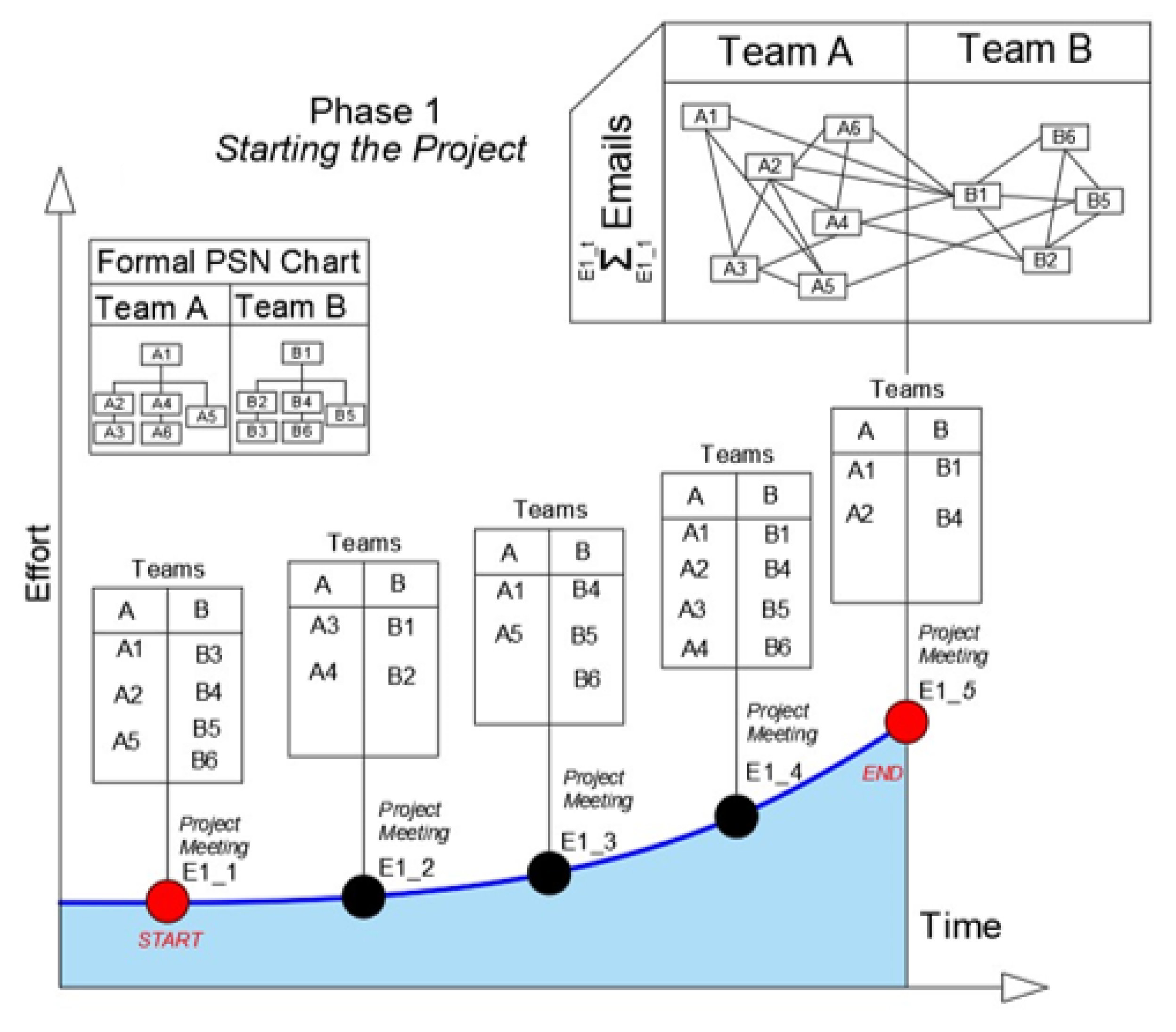
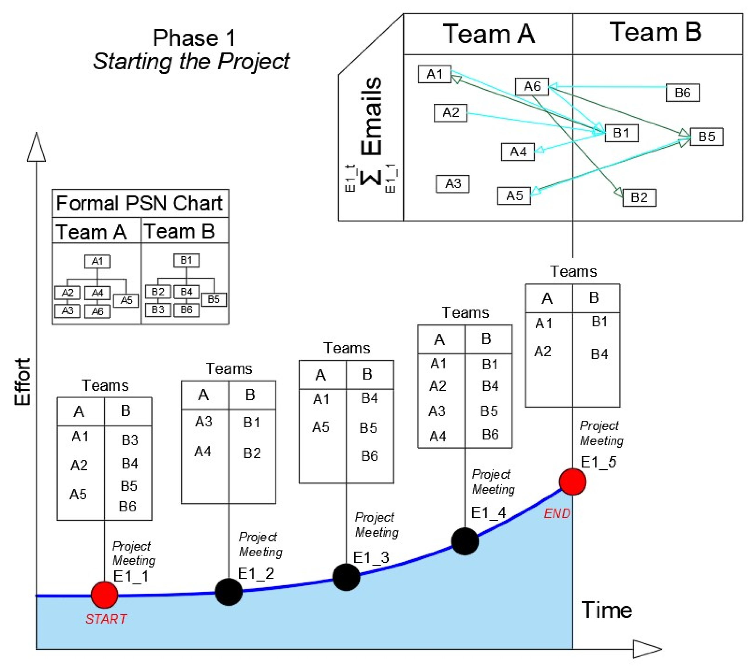
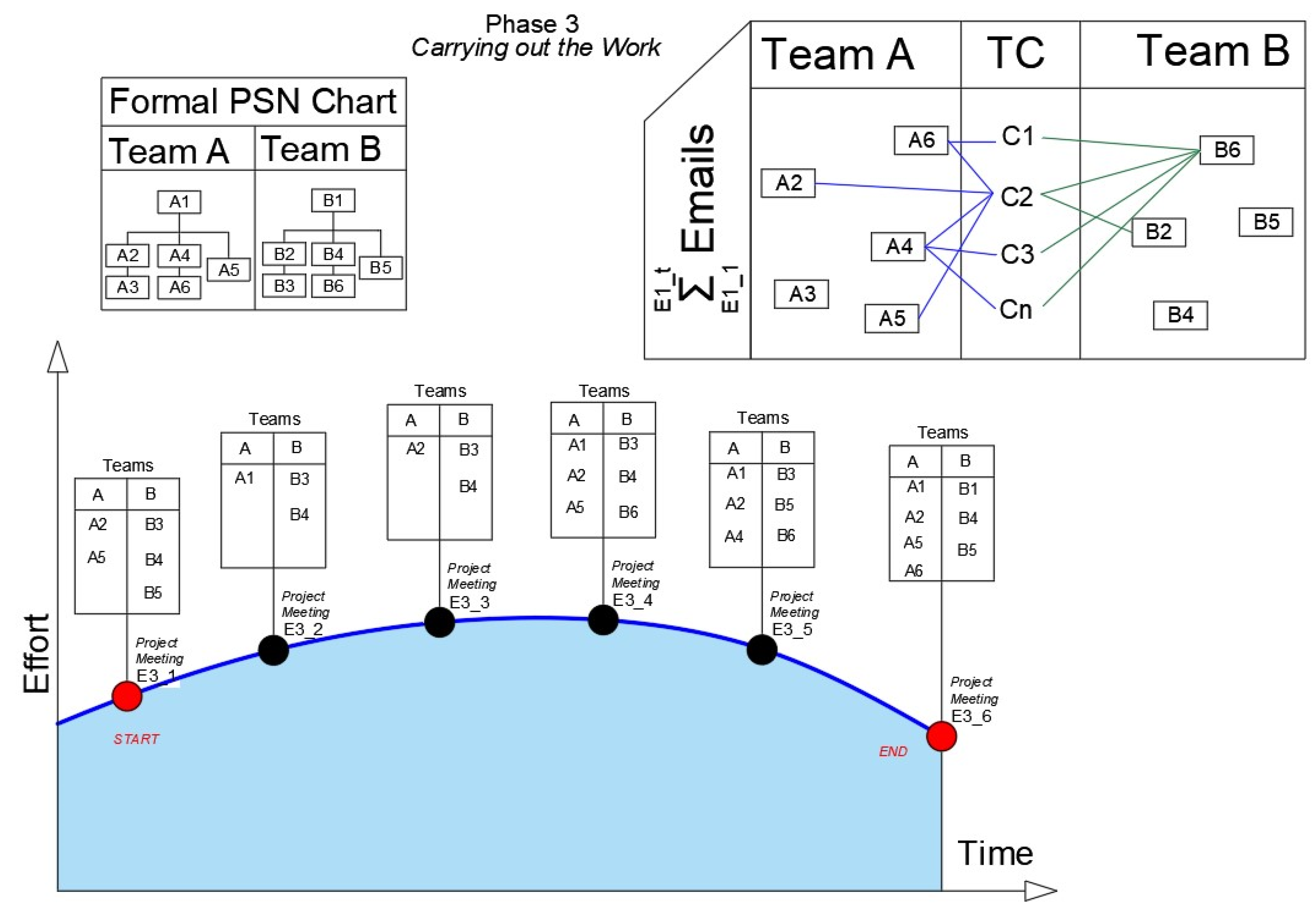
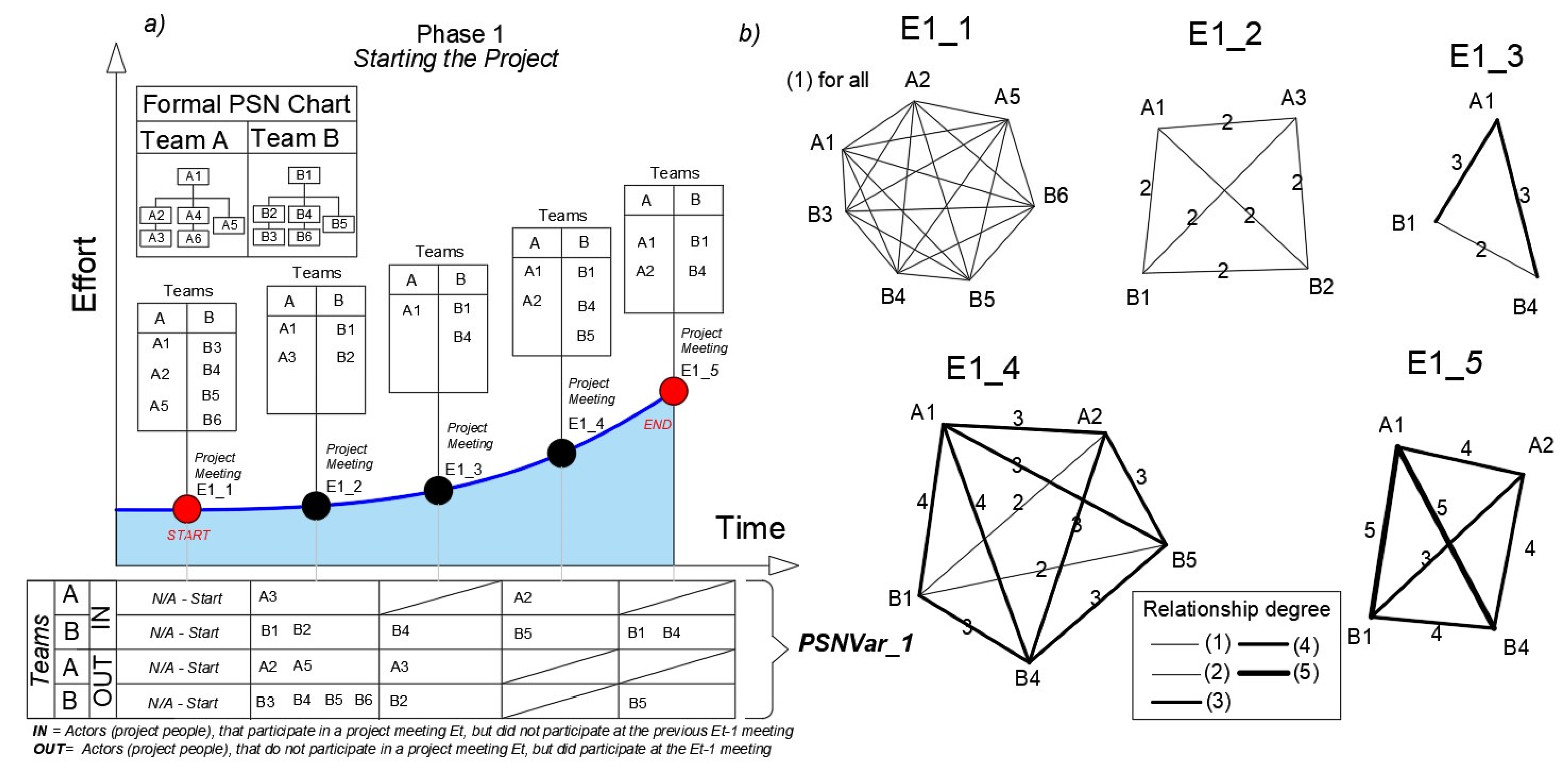
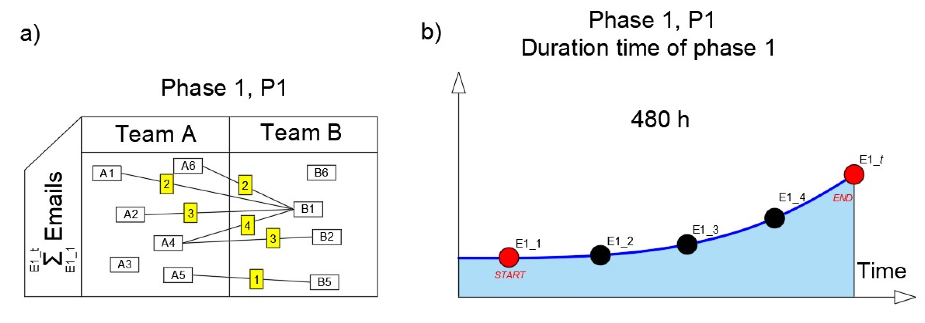
4.2. Case Study
4.2.1. Role Attendee Degree
4.2.2. Internal Mail Cohesion Degree
- LM = total number of existing links at the email communication network
- NM = total number of project people connected, within the email communication network
First Approach
Second Approach
- TD = total degree in the email communication network
- NM = total number of project people connected within the email communication network
- i = project person = 1, 2, 3, …, NM
- NM_li = total number of existing links attached to project person i
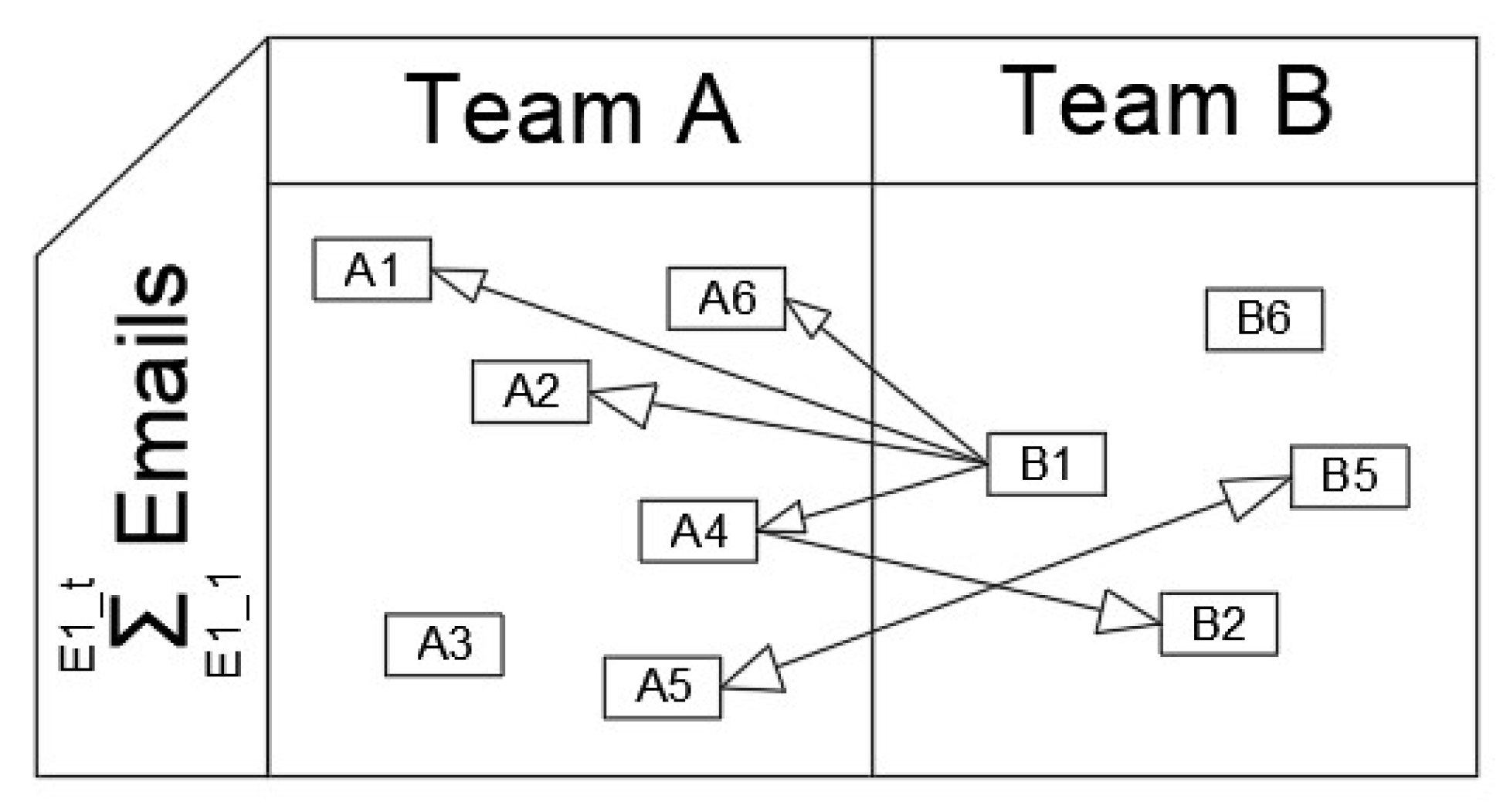
4.2.3. Feedback Degree
- ID = In-degree in the email communication network
- NM = total number of project people connected, within the email communication network
- i = project person = 1, 2, 3, …, NM
- NM_lin = total number of existing in-links attached to project person i
| ID(A1) = 1 ID(A2) = 1 ID(A3) = 0 ID(A4) = 1 ID(A5) = 1 ID(A6) = 1 | ID(B1) = 0 ID(B2) = 1 ID(B5) = 1 ID(B6) = 0 |
- OD = Out-degree in email communication network
- NM = total number of project people connected, within the email communication network
- i = project person = 1, 2, 3, …, NM
- NM_lout = total number of existing out-links attached to project person i
| OD(A1) = 0 OD(A2) = 0 OD(A3) = 0 OD(A4) = 1 OD(A5) = 1 OD(A6) = 0 | OD(B1) = 4 OD(B2) = 0 OD(B5) = 1 OD(B6) = 0 |
- RM = Reciprocity in email communication network
- Sent Mails low = sum of the lowest number of emails sent by one given team
- Sent Mails high = sum the highest number of emails sent by one given team
4.2.4. Information Seeking/Providing Degree
4.2.5. Action Key Players
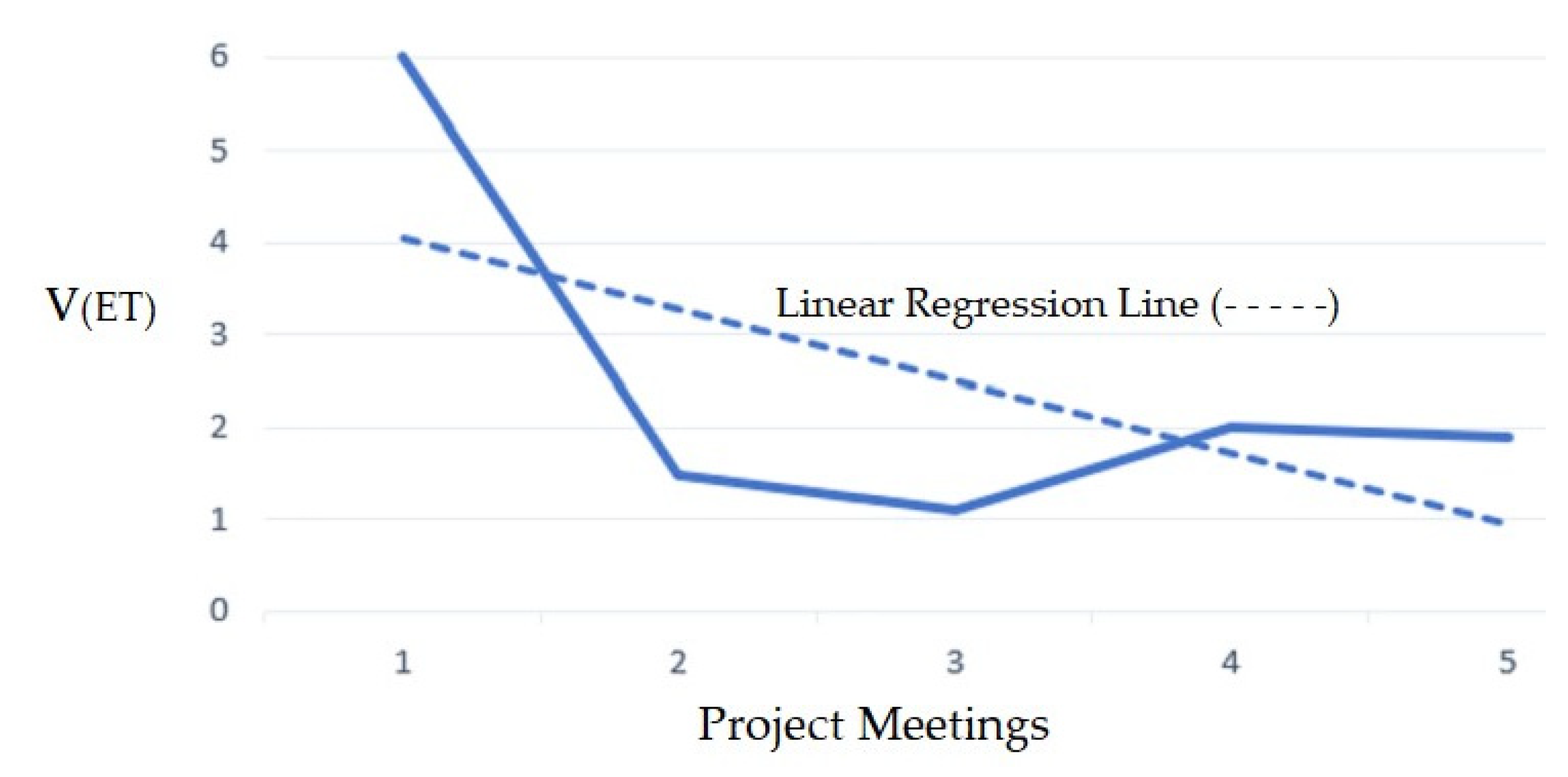
4.2.6. Meetings Cohesion Degree
- V = Variability of a PSN (project social network)
- Et = Meeting (event) number, where Et = 1, 2, …, TE
- TE = Number of project meetings (events) that occurred in a given project phase TPP = Number of project person that participated in an event Et.
- WL = Value of all weighed connections (links), from each project stakeholder total degree in each project meeting (event) Et.
4.2.7. Teamwork Performance
- = Sum of all times from all replied to emails within a project phase.
- TCMs = Total of emails sent and replied within the email network communication
5. Discussion
6. Conclusions
Author Contributions
Funding
Institutional Review Board Statement
Informed Consent Statement
Data Availability Statement
Conflicts of Interest
References
- Nunes, M.; Abreu, A. Applying Social Network Analysis to Identify Project Critical Success Factors. Sustainability 2020, 12, 1503. [Google Scholar] [CrossRef] [Green Version]
- Brass Daniel, J.; Borgatti Stephen, P. Social Networks at Work (SIOP Organizational Frontiers Series), 1st ed.; Routledge Publisher: New York, NY, USA, 2020. [Google Scholar]
- Abreu, A.; Nunes, M. Model to Estimate the Project Outcome’s Likelihood Based on Social Networks Analysis. KnE Eng. 2020, 5, 299–313. [Google Scholar] [CrossRef]
- Arena, M.; Cross, R.; Sims, J.; Uhl-Bien, M. How to Catalyze Innovation in Your Organization. 2017. Available online: https://www.robcross.org/wp-content/uploads/2020/03/SMR-how-to-catalyze-innovation-in-your-organization-connected-commons.pdf (accessed on 9 January 2022).
- Nunes, M.; Abreu, A. The Benefits of Applying Social Network Analysis to Identify Collaborative Risks. In Technological Innovation for Applied AI Systems. DoCEIS 2021. IFIP Advances in Information and Communication Technology, Caparica, Portugal, 7–9 July 2021; Camarinha-Matos, L.M., Ferreira, P., Brito, G., Eds.; Springer: Cham, Switzerland, 2021; Volume 626. [Google Scholar]
- Workday Studios. Good Company—Michael Arena, Chris Ernst, Greg Pryor: Organizational Networks. 2018. Available online: https://www.youtube.com/watch?v=6faV0v0yVFU (accessed on 12 January 2022).
- Nunes, M.; Abreu, A. Applying social network analysis to support the management of cooperative project’s behavioral risks. FME Trans. 2021, 49, 795–805. [Google Scholar] [CrossRef]
- Arena, M. Adaptive Space: How GM and Other Companies are Positively Disrupting Themselves and Transforming into Agile Organizations; McGraw Hill Education: New York, NY, USA, 2018. [Google Scholar]
- Wasserman, S.; Faust, K. Social Network Analysis in the Social and Behavioral Sciences. In Social Network Analysis: Methods and Applications; Cambridge University Press: Cambridge, MA, USA, 1994; pp. 1–27. ISBN 9780521387071. [Google Scholar]
- Krackhardt, D.; Hanson, J. Informal Networks the Company behind the Charts; Harvard College Review: Cambridge, MA, USA, 1993; Available online: https://hbr.org/1993/07/informal-networks-the-company-behind-the-chart (accessed on 5 February 2022).
- Freeman, L. Centrality in social networks conceptual clarification. Soc. Netw. 1979, 1, 215–239. [Google Scholar] [CrossRef] [Green Version]
- Leonardi, P.; Contractor, N. Better People Analytics; Harvard Business Review. Available online: https://hbr.org/2018/11/better-people-analytics (accessed on 15 February 2022).
- Nunes, M.; Abreu, A. Managing Open Innovation Project Risks Based on a Social Network Analysis Perspective. Sustainability 2020, 12, 3132. [Google Scholar] [CrossRef]
- Cross, R.; Rebele, R.; Grant, A. Collaborative Overload. Harv. Bus. Rev. 2016, 94, 74–79. [Google Scholar]
- Nunes, M.; Abreu, A.; Bagnjuk, J.; Tiedtke, J. Measuring project performance by applying social network analyses. Int. J. Innov. Stud. 2021, 5, 35. [Google Scholar] [CrossRef]
- Ng, D.; Law, K. Impacts of informal networks on innovation performance: Evidence in Shanghai. Chin. Manag. Stud. 2015, 9, 56–72. [Google Scholar] [CrossRef]
- PMI®. Project Management Body of Knowledge (PMBOK® Guide), 6th ed.; Project Management Institute, Inc.: Newtown Square, PA, USA, 2017; pp. 10–11. [Google Scholar]
- The Standish Group International, Inc. CHAOS REPORT 2015. Available online: https://www.standishgroup.com/sample_research_files/CHAOSReport2015-Final.pdf (accessed on 1 February 2022).
- Tereso, A.; Ribeiro, P.; Fernandes, G.; Loureiro, I.; Ferreira, M. Project Management Practices in Private Organizations. Proj. Manag. J. 2019, 50, 6–22. [Google Scholar] [CrossRef]
- Nunes, M.; Abreu, A.; Bagnjuk, J. A Model to Manage Organizational Collaborative Networks in a Pandemic (COVID-19) Context. In Smart and Sustainable Collaborative Networks 4.0. PRO-VE 2021. IFIP Advances in Information and Communication Technology, France, 22–24 November; Camarinha-Matos, L.M., Boucher, X., Afsarmanesh, H., Eds.; Springer: Cham, Switzerland, 2021; Volume 629. [Google Scholar]
- Project Performance Metrics. Reprinted from PMI’s Pulse of the Profession 9th Global Project Management Survey, by Project Management Institute. 2017. Available online: https://www.pmi.org//media/pmi/documents/public/pdf/learning/thought-leadership/pulse/pulse-of-the-profession-2017.pdf and https://www.pmi.org/annual-report-2019/highlights (accessed on 1 January 2022).
- The Standish Group International, Inc. Project Resolution Benchmark Report—Jennifer Lynch—2018. Available online: https://www.standishgroup.com/sample_research_files/DemoPRBR.pdf and https://www.infoq.com/articles/standish-chaos-2015/ (accessed on 1 February 2022).
- Nunes, M.; Abreu, A.; Saraiva, C. Identifying Project Corporate Behavioral Risks to Support Long-Term Sustainable Cooperative Partnerships. Sustainability 2021, 13, 6347. [Google Scholar] [CrossRef]
- Saraiva, C.; Mamede, H.S.; Silveira, M.C.; Nunes, M. Transforming physical enterprise into a remote organization: Transformation impact: Digital tools, processes, and people. In Proceedings of the 2021 16th Iberian Conference on Information Systems and Technologies (CISTI), Madrid, Spain, 22–25 June 2021; pp. 1–5. [Google Scholar]
- Hillson, D. The Risk Doctor—Speaker at Risk Zone 2012. Stamford Global. Available online: https://www.youtube.com/watch?v=0d3y863itjk (accessed on 1 January 2022).
- Nunes, M.; Bagnjuk, J.; Abreu, A.; Saraiva, C.; Nunes, E.; Viana, H. Achieving Competitive Sustainable Advantages (CSAs) by Applying a Heuristic-Collaborative Risk Model. Sustainability 2022, 14, 3234. [Google Scholar] [CrossRef]
- Carroll, N.; Whelan, E.; Richardson, I. Applying Social Network Analysis to Discover Service Innovation within Agile Service Networks. Serv. Sci. 2010, 2, 225–244. [Google Scholar] [CrossRef] [Green Version]
- Lee, C.; Chong, H.Y.; Liao, P.; Wang, X. Critical Review of Social Network Analysis Applications in Complex Project Management. J. Manag. Eng. 2018, 34, 04017061. [Google Scholar] [CrossRef] [Green Version]
- Nunes, M.; Abreu, A.; Bagnjuk, J.; D’Onfrio, V.; Saraiva, C. A Heuristic Model to Identify Organizational Collaborative Critical Success Factors (CSFs). In Proceedings of the 2021 6th International Young Engineers Forum (YEF-ECE), Caparica, Portugal, 9 July 2021; pp. 63–68. [Google Scholar]
- Scott, J. Social Network Analysis: A Handbook, 4th ed.; SAGE: Thousand Oaks, CA, USA, 2017. [Google Scholar]
- De Brun, A.; McAuliffe, E. Social Network Analysis as a Methodological Approach to Explore Health Systems: A Case Study Exploring Support among Senior Managers/Executives in a Hospital Network. Int. J. Environ. Res. Public Health 2018, 15, 511. [Google Scholar] [CrossRef] [PubMed] [Green Version]
- Waber, B. Using Analytics to Measure Interactions in the Workplace | Ben, Humanyze, Founder & CEO—Sociometric Badges. 2014. Available online: https://hd.media.mit.edu/badges/ - https://www.youtube.com/watch?v=XojhyhoRI7I (accessed on 1 January 2022).
- Borgatti, S. Introduction to Social Network Analysis Stephen, University of Kentucky. 2016. Available online: https://statisticalhorizons.com/wp-content/uploads/SNA-Sample-Materials.pdf (accessed on 15 January 2022).
- Ulrik, B.; Borgatti, S.; Freeman, C. Maintaining the duality, of closeness and betweenness centrality. Soc. Netw. 2016, 44, 153–159. [Google Scholar] [CrossRef] [Green Version]
- Albert, R.; Barabási, A. Statistical mechanics of complex networks. Rev. Mod. Phys. 2002, 74, 47–97. [Google Scholar] [CrossRef] [Green Version]
- Xing, S. Dynamic Social Network Analysis: Model, Algorithm, Theory, & Application CMU Research Speaker Series. 2016. Available online: https://www.youtube.com/watch?v=uiD988ISE3o (accessed on 15 March 2022).
- Dogan, S.; Arditi, D.; Gunhan, S.; Erbasaranoglu, B. Assessing Coordination Performance Based on Centrality in an E-mail Communication Network. J. Manag. Eng. 2013, 31, 04014047. [Google Scholar] [CrossRef] [Green Version]
- Wen, Q.; Qiang, M.; Gloor, P. Speeding up decision-making in project environment: The effects of decision makers’ collaboration network dynamics. Int. J. Proj. Manag. 2018, 36, 819–831. [Google Scholar] [CrossRef]


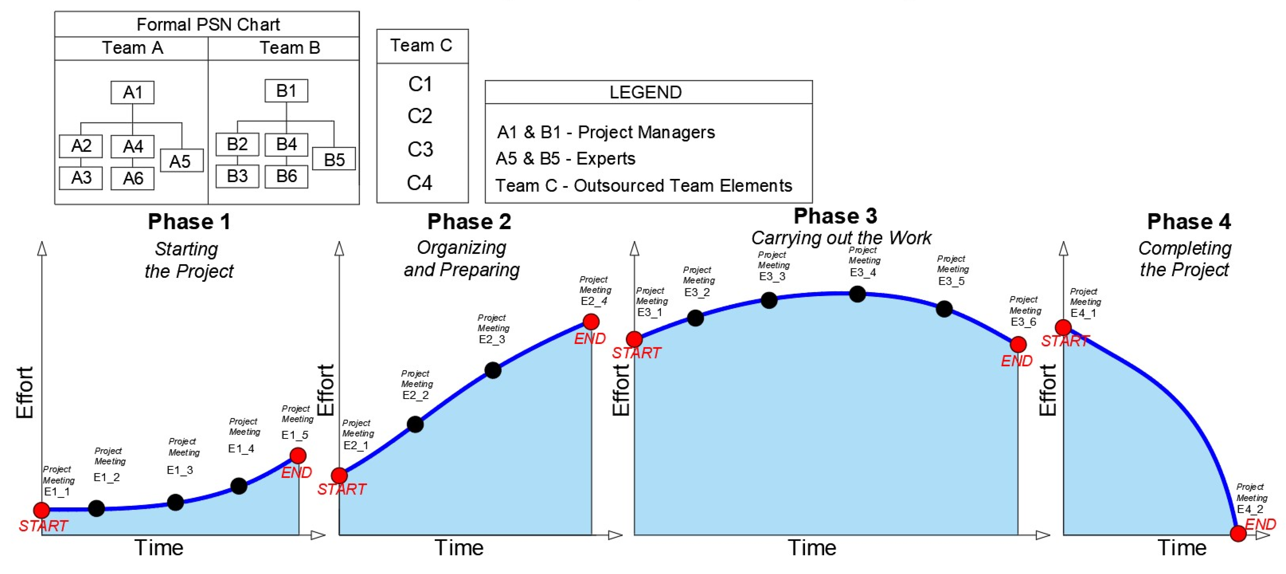
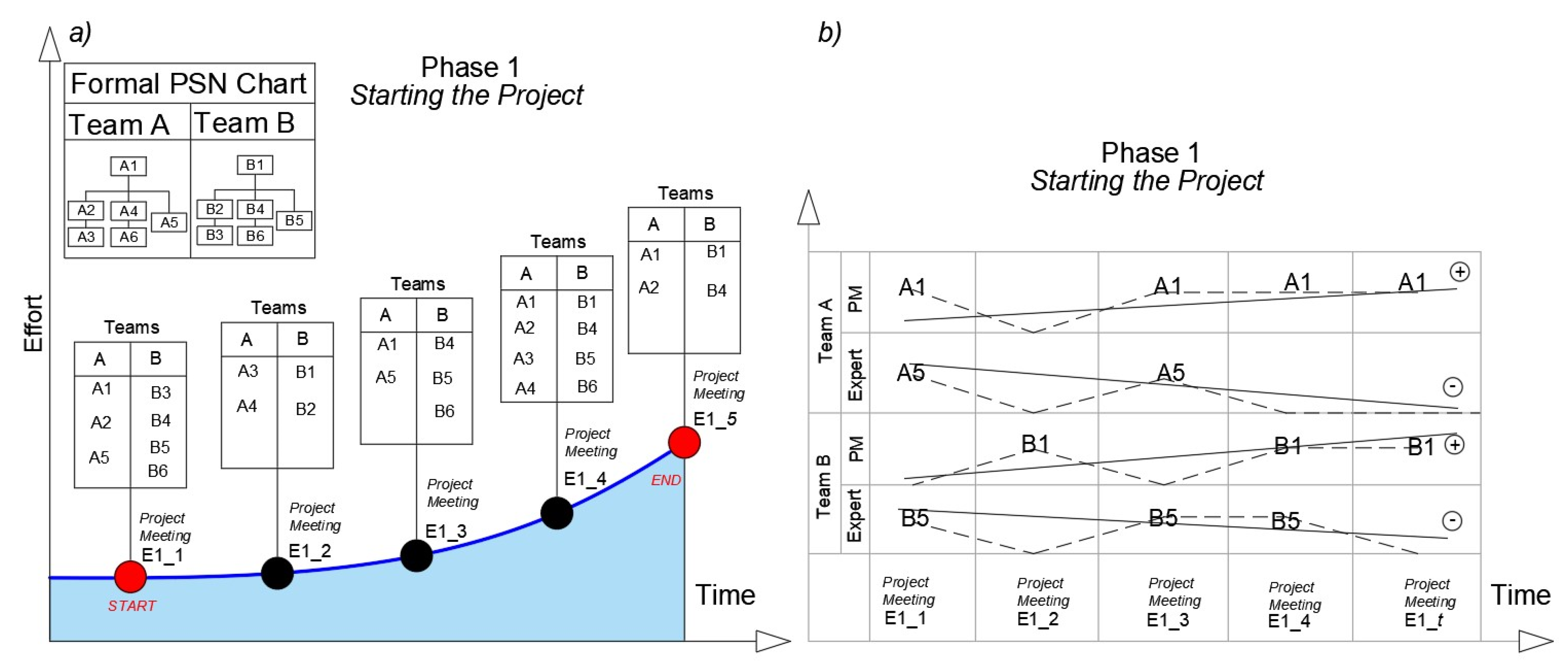
| Year | Event | Description |
|---|---|---|
| 1930–1953 | Formulation of graph theory by Jewish-Hungarian mathematician Dénes König. | Publishing of the König’s Book—Theorie der endlichen und unendlichen Graphen—in USA. König’s ideas started to be developed by Haary and Norman, and since then, began to be applied to study Social Networks [27,28,29,30,31,32]. |
| 1940–1950 | Development of three most important graph-based metrics: (1) In-degree, (2) out-degree, and (3) total degree. | Psychologists Leavitt, Bavelas, and Smith in 1950 developed three of the most popular centrality measures [1,4,8]. These are used to measure how many links or preferences one entity (person, group, or organization) receives or gives from or to other actors of the social network where they exist. |
| 1950–1970 | Development of Betweenness centrality. | Started to be developed in the late 1940’s by Cohn and Marriott, was finalized in the late 1970’s by Anthonisse (1971), Freeman (1977), and Pitts (1979) [9,33]. Betweenness Centrality calculates the shortest path between every pair of nodes in a connected graph, and it can be used to describe the amount of influence that an entity has over the flow of information in a network. It is also often used to find entities that serve as a bridge between two different blocks of a network [9,33]. |
| 1960–1975 | Development of Closeness centrality. | Closeness centrality was developed followed the works of Bavelas in 1950, Harary in 1959, by Beauchamp in 1965, and Sabidussi in 1966, and finalized by Moxley and Moxley and Rogers in 1974. It measures how close one entity is to all the other entities within a network [9,33]. |
| 1970–1980 | Development of Density. | Another popular centrality measure that are used to characterize group cohesion is the Density. Started by Bott in 1957 and finalized in 1980 by Thurman, it represents how strongly or how weakly a network is connected regarding the number of links between entities, which represents how far an entity can reach another entity through a set of intermediate links [9,33]. |
| 2000–2017 | Redevelopment of the centrality concept in graph-based theory | The latest research argues that the centrality concept needs to be revised and should not be uniquely dependent on the position of an entity in a network as Sabidussi in 1966 and Freeman in 1979 proposed [33,34]. Such redevelopment stated that some centrality metrics in isolation may be inefficient to explain dynamic behavior. They argue that the nature of work that the entities execute should also be added when analyzing dynamic behaviors or that centrality metrics should be supported by some type of other metrics from other scientific areas [33,34]. |
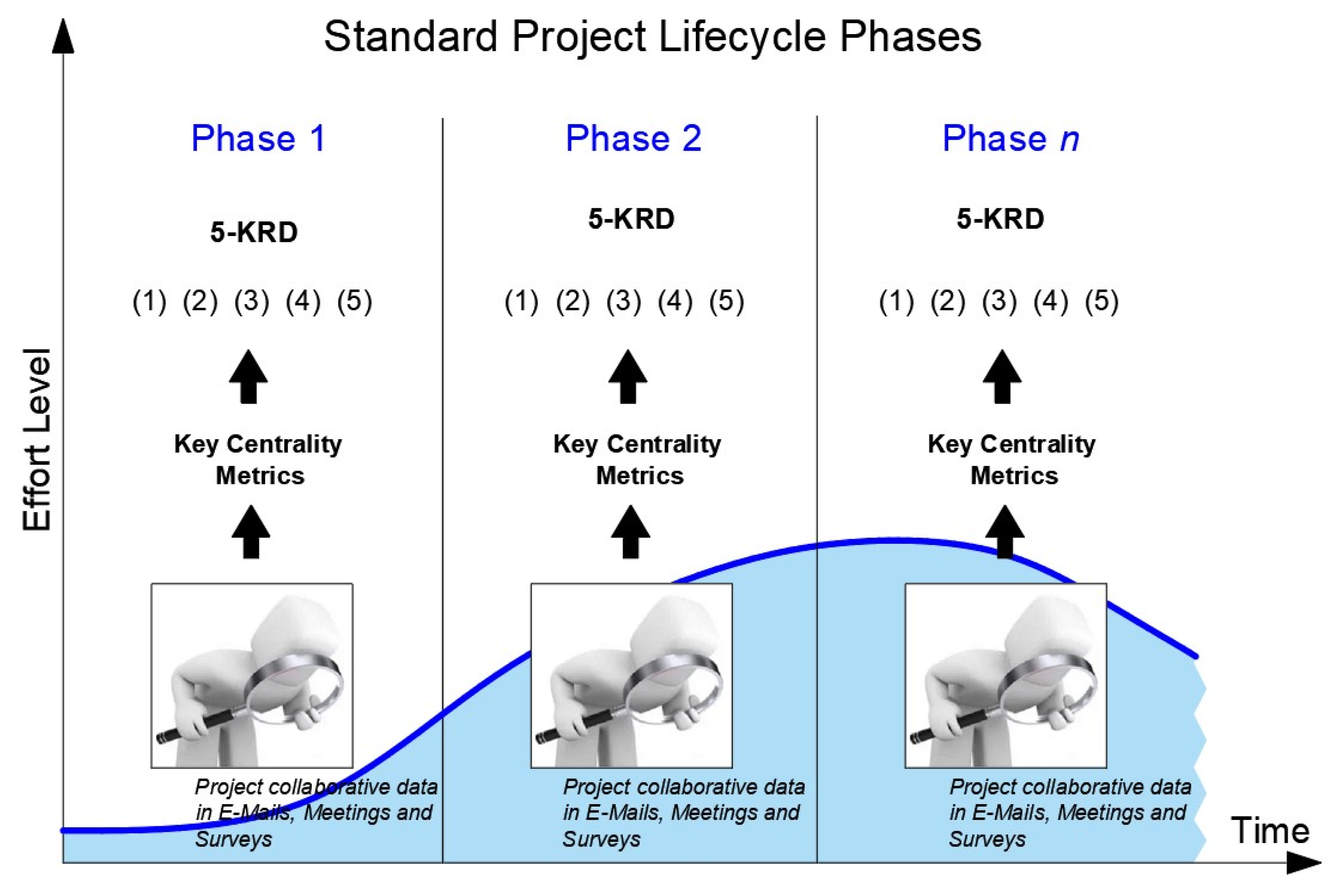
| 1- Communication | How do project roles, such as project managers, experts, engineers, or project administrative roles, communicate and the respective consequences of such communication behavioral patterns? Topics such as reach, strong or weak feedback, and the presence of project roles in project meetings are suitable to be analyzed. |
| 2- Internal and external collaboration | How strong is the dependency level regarding project-related information between any two given project teams or groups? What level of collaboration (collaborative overload or lack of collaboration) is practiced in a project social network? |
| 3- Know-how exchange and informal power | How is project-related information shared across the different project stakeholders of a project social network? How do influential informal and usually invisible project stakeholders influence decision-making and the execution of tasks and project activities? |
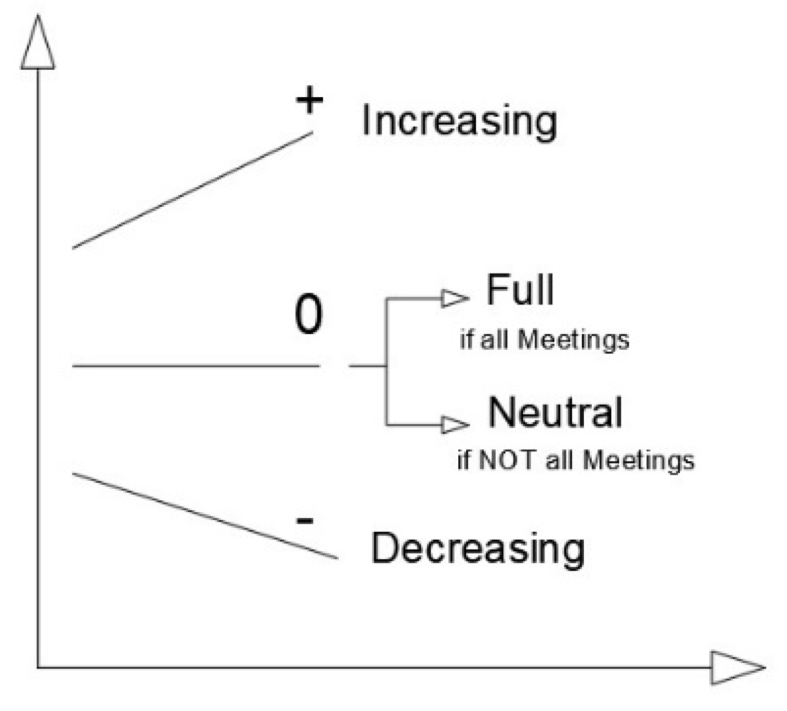
| 4- Team-set variability | How does the variability of a project team-set impact project outcome? Does an unchangeable team set from the beginning until the end of a project help to achieve more project success than a continuously changing project team set? |
| 5- Teamwork performance | How is the level of project team performance measured in feedback replies regarding important project information? |
| PEIC | Necessary Data for Proposed Metrics |
|---|---|
| Project Meetings (Events) | Number of conducted project meetings in each one of the phases of a project lifecycle Number of participant project stakeholders in each one of the project meetings Project role name and to which team the respective project role belongs |
| Project Exchanged Mails | Number of exchanged emails sent/received in each one of the phases of a project lifecycle that regards project related information. Emails are organized as follows:
|
| Project Surveys (Questionnaires) | Conduct a simple social network analysis assessment by applying pre-defined questions that uncover important project-related information. Questions can be as follows:
|
| Sources Metrics | PEICs | |||||
|---|---|---|---|---|---|---|
| Data from Meetings | Data from Mails | Data from Questionnaires | First Measurement | Second Measurement | 5-KRD (Five Global Collaboration Types) | |
| Metric M1-Role attendee degree | x | SNA: Total In-degree | Statistics: Linear Regression | Communication | ||
| Metric M2-Internal mail cohesion degree | x | SNA: Total degree and Density | Statistics: Average | |||
| Metric M3-Feedback degree | x | SNA: In-degree and Out-degree and Reciprocity | Statistics: Mode | |||
| Metric M4-Information Seeking/Provide degree | x | SNA: In-degree and Out-degree | Statistics: Mode | Internal and external collaboration | ||
| Metric M5-Action key players | x | SNA: Total In-degree | Statistics: Mode | Know-how exchange and informal power | ||
| Metric M6-Meeting’s cohesion degree | x | SNA: Average weighted total-degree | Statistics: Linear Regression | Team set variability | ||
| Metric M7-Teamwork performance | x | SNA: Total In-degree | Statistics: Average | Teamwork performance | ||
| Metrics Number | Independent PSN Stakeholders | Global PSN Stakeholders | ||
|---|---|---|---|---|
| Project Managers | Experts | Outsourcers | All Official Defined Project Roles (Team A and Team B) | |
| Metric M-1 | x | x | ||
| Metric M-2 | x | x | x | |
| Metric M-3 | x | |||
| Metric M-4 | x | |||
| Metric M-5 | x | x | ||
| Metric M-6 | x | |||
| Metric M-7 | x | |||
| Team A | Team B | |||
|---|---|---|---|---|
| Project Manager (A1) | Expert (A5) | Project Manager (B1) | Expert (B5) | |
| Total Degree | 3 | 4 | 7 | 4 |
| Blue Color | Team A | Team B |
|---|---|---|
| Team A | - | 3 |
| Team B | 3 | - |
| Green Color | Team A | Team B |
|---|---|---|
| Team A | - | 3 |
| Team B | 1 | - |
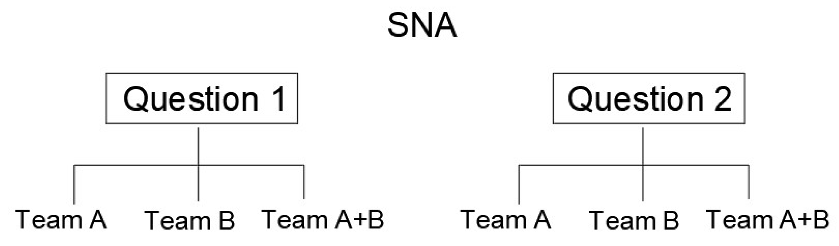
| Question 1 (In-Degree) | Question 2 (In-Degree) | ||
|---|---|---|---|
| A2 | 1 | A2 | 0 |
| A3 | 0 | A3 | 0 |
| A4 | 3 | A4 | 0 |
| A5 | 1 | A5 | 0 |
| A6 | 0 | A6 | 0 |
| B2 | 1 | B2 | 0 |
| B4 | 0 | B4 | 0 |
| B5 | 0 | B5 | 0 |
| B6 | 0 | B6 | 4 |
| B1 | B2 | B5 | ||||||
|---|---|---|---|---|---|---|---|---|
| A1 | 1 | 1 | ------ | ------ | ------ | ------ | ------ | ------ |
| A2 | 0.3 | 0.4 | 0.8 | ------ | ------ | ------ | ------ | ------ |
| A4 | 0.1 | 1 | 0.3 | 1 | 0.3 | 1 | 0.8 | ------ |
| A5 | ------ | ------ | ------ | ------ | ------ | ------ | ------ | 0.1 |
| A6 | 0.2 | 0.8 | ------ | ------ | ------ | ------ | ------ | ------ |
Publisher’s Note: MDPI stays neutral with regard to jurisdictional claims in published maps and institutional affiliations. |
© 2022 by the authors. Licensee MDPI, Basel, Switzerland. This article is an open access article distributed under the terms and conditions of the Creative Commons Attribution (CC BY) license (https://creativecommons.org/licenses/by/4.0/).
Share and Cite
Nunes, M.; Bagnjuk, J.; Abreu, A.; Cardoso, E.; Smith, J.; Saraiva, C. Creating Actionable and Insightful Knowledge Applying Graph-Centrality Metrics to Measure Project Collaborative Performance. Sustainability 2022, 14, 4592. https://doi.org/10.3390/su14084592
Nunes M, Bagnjuk J, Abreu A, Cardoso E, Smith J, Saraiva C. Creating Actionable and Insightful Knowledge Applying Graph-Centrality Metrics to Measure Project Collaborative Performance. Sustainability. 2022; 14(8):4592. https://doi.org/10.3390/su14084592
Chicago/Turabian StyleNunes, Marco, Jelena Bagnjuk, António Abreu, Edgar Cardoso, Joana Smith, and Célia Saraiva. 2022. "Creating Actionable and Insightful Knowledge Applying Graph-Centrality Metrics to Measure Project Collaborative Performance" Sustainability 14, no. 8: 4592. https://doi.org/10.3390/su14084592