Impact of Government Stability and Investment Profile on Forest Area: The Role of Natural Protected Areas

Abstract

Forest area plays a fundamental role in air and water quality and directly impacts agricultural productivity. This research aims to examine the impact of government stability and investment profiles on forest cover in countries within the ASEAN region. Specifically, the research includes Brunei Darussalam, Indonesia, Malaysia, Myanmar, the Philippines, Singapore, Thailand, and Vietnam. In the research development, we examine the role which protected natural areas play in the conservation of forests. We employ second-generation cointegration methods of cross-section dependence and slope heterogeneity. The results suggest that forest cover has been significantly reduced in this region, while government stability and the investment profile have a volatile behavior. The second-generation cointegration test results suggest there is no long-term relationship between the three series. Likewise, the short- and long-term elasticities highlight the importance of environmental protection policies to conserve forests.

1. Introduction

The conservation of natural areas in the ASEAN region is relevant due is one of the few regions where the variable is decreasing. Over time, a series of policies have been implemented to promote the conservation of forest cover. The ASEAN region has one of the highest rates of deforestation explained by the felling of natural forests, urbanization, habitat fragmentation, and the expansion of the agricultural frontier, causing species extinction [1,2]. Likewise, factors such as the expansion of industries generated by high demands for food have endangered the protected areas of countries of Southeast Asia, reducing forest areas [3,4]. The need for reforestation policies, the introduction of native species, and the preservation of forest extensions contribute to the conservation of the various natural areas. The strictest environmental regulations in the countries allow ecosystem services and biodiversity conservation and improve long-term sustainability [5].

The importance of protected natural areas plays a relevant role in conserving the natural habitat that is essential for the water cycle and purifying the air. However, environmental education is necessary for the population, to empower them to conserve forests. The protection of the marine areas of Nha Trang Bay and Cu Lao Cham in Vietnam has been maintained due to economic incentives that favor the transition to conservation behaviors. However, situations such as the influence of market forces in the tourism and fishing sector have generated low biodiversity conservation [6]. These authors emphasize that the inefficient intervention of the government, together with other problems of the country, hinders the sustainable use of natural resources. Con Dao National Park was one of the first protected areas in Vietnam. Despite this, globalization through trade liberalization and low government control has led to poor ecosystem resource management [7]. These authors suggest that the government improves capacity through legal frameworks, transparency, coordination with other entities, and community participation. In addition, improvements in institutionality allow environmental conservation to be included in developing policies that encourage foreign capital inflows to maximize economic growth.

One of the arguments most used by farmers or forest owners is that the economic activities associated with forest management are the means of subsistence. This fact conditions the forests’ management so that the rural population can subsist. However, payment for conservation is a widely applied policy in various contexts, with heterogeneous results. In Vietnam, the Payment for Forest Environmental Services policy was proposed to renew forest resource management in the Muong Nhe protected area located in Dien Bien, and was applied in 2011. Its results revealed that the impacts of the policy on large communities are positive by promoting greater forest management and protection [8]. Similarly, it contributed to the conservation of forests with a greater awareness of the population. In the Nusa Penida protected area in Indonesia, it was highlighted that low governance responsibility and inefficient state action reduced the strength of incentives to protect this area [9]. Likewise, in the Weh Island Marine Recreational Park (WMRP) and the Weh Island Marine Protected Area (WMPA), it was found that the community does not trust the government and ensures that the support of the interested parties is more effective to achieve environmental care [10,11,12]. Moreover, it has been revealed that with the increase of governance mechanisms through community incentives, it will be possible to assume an active role in managing protected areas in Indonesia’s conserving ecosystems [13]. The anti-deforestation policy, implemented in Indonesia in 2011, demonstrated the loss of forests from several protected areas felling more than 1000 square kilometers (km²) of forests in a relatively short time. This occurred due to the transfer of productive activities in the various areas, producing additional forest losses [14]. In general, an obstacle to forest conservation is the unsustainable economic activities of the population. This fact justifies the need to increase society’s knowledge about the importance of forest conservation.

On the other hand, in Malaysia, it is highlighted that co-management in the management of protected areas and natural resources is vital for their conservation. Therefore, the government’s coordination, cooperation, and collaboration with the community provide a series of benefits for vegetation cover [15]. In Myanmar, an ASEAN country, it was indicated that policies and greater management planning help take better care of parks and protected areas [16]. The economic benefits obtained from the administration of resources in areas of Myanmar, however, lag behind decision-making for their conservation. Therefore, the evaluation of the services provided by ecosystems allows for proposing strategies for sustainable management [17]. Among others, Myanmar’s biodiversity is threatened by various factors, including deforestation, population growth, indiscriminate burning, and mining. In this economy, 26.8% of the habitat corresponds to protected areas that are more exposed to vulnerable situations [18].

In parallel, in recent decades, several countries in the ASEAN region have implemented policies to improve the environment to encourage inflows of foreign direct investment and increase economic growth. However, economic growth policies are not exempt from economic consequences, both short and long term. The improvements in the economic environment include legal reforms to improve the institutional framework and give stability to the government to favor increases in investment. Against this background, our research examines the impact of government stability and investment profile on forest cover in countries within the ASEAN region. The data characteristics show that the series depends on the cross-sections, and there is heterogeneity on the slope. We obtained this result by using the Pesaran test [19], and Pesaran and Yamagata [20] suggest the need to estimate the unit root tests and the second-generation cointegration test. Specifically, we employ the Herwartz and Siedenburg [21], Pesaran [22], and Breitung [23] tests. Finally, we estimate the strength of the cointegration vector using the fully modified ordinary least squares (FMOLS) method and the short- and long-run elasticities using the augmented mean group estimator (AMG) and the common correlated effects mean group estimator (CCE-MG) models. The results support the need to improve institutional policies to conserve forests and thus achieve the sustainability of these economies.

The remaining of the investigation is organized as follows. The second section develops the review of the literature, with emphasis on the institutional factors that affect forest cover. The third section reports on the sources and characteristics of the data. The fourth section outlines the methodological strategy used to verify the hypotheses. The fifth section reports the results, discussing the findings with the previous literature. Finally, the sixth section presents the conclusions of the research and the implications for environmental policy.

2. Literature Review

The protection of the environment represents one of the most relevant objectives in the sustainable development agenda [24]. However, the scarcity of natural resources raises concerns about their possible harmful effect on the productive capacities of nature [25]. Structural changes related to institutionality can help understand the dynamics of the environmental Kuznets curve (EKC). One of the obstacles to understanding the totality of the environmental dynamics has focused on analyzing the production of an economy without considering the sustainability of nature [26]. Economic activity includes both the production process and the consumption process. Furthermore, demand drives all goods’ production, purchases, and sales [27]. Therefore, the EKC concept presupposes that the production base of an economy changes gradually and over time from agriculture to industry and, subsequently, to services [28]. Finally, the relationship between income and environmental pollution takes the form of an inverted U [29]. The nexus between environmental degradation and economic development has been limited to air pollution and the ecological footprint [30,31]. However, the need to improve the understanding of environmental degradation implies including new ways of measuring environmental sustainability.

According to the EKC theory, the process of economic growth is expected to ultimately lessen the environmental degradation created in the early stages of development [32]. Next, Vincent [33] points out that both developing and developed countries have different EKC curve sides. In this logic, developing countries are in the ascending section of the EKC, while developed countries are in the descending section [34]. Likewise, Roberts and Grimes [35] indicated that an EKC pattern is valid only for high-income countries just before the two oil shocks in the 1970s. Only a relatively small number of developed countries become more energy efficient; while the efficiency of the rest of the world worsens [36]. Grossman and Krueger [37] estimated that income has the most consistent significant effect on most environmental quality indicators. The empirical findings implied that a country could overcome its environmental problems. However, this process is not automatic but instead requires institutional aspects directed from pro-environmental policies [8]. In this sense, policies aimed at conserving nature and, more specifically, forest cover, it is necessary to create protected natural forests through legal and fiscal mechanisms [13]. Creating protected natural areas has significantly improved forest conservation and has limited economic activity in protected forests [17]. Countries in the ASEAN region have experienced rapid economic growth, stemming from substantial foreign direct investment. This fact implies that the environmental quality measured by the forest cover has experienced an impact that has influenced its temporal behavior.

Regarding the pollution paradise hypothesis, Kaika and Zervas [38] state that developing countries have grown enough and will face severe environmental degradation in the future. This problem will cause these countries to substitute their pollution-intensive domestic production for imports from other developing countries with less stringent environmental regulations. For his part, Cole [39] points out that if the demand for pollution-intensive goods from developed countries continues to be satisfied with imports from developing countries, then the latter will not transfer this production of pollution-intensive goods to other developing countries. On the contrary, Wagner [40] indicates that developed countries may have become more energy efficient, and their pollution-intensive production may have migrated to poorer countries. However, this does not imply that their preferences have changed because they continue to consume energy-intensive goods. Finally, regarding the pollution haven hypothesis, Ngarambe et al. [41] explain how multinational companies that participate in activities cause pollution and move their production lines to low-income countries with weak environmental standards.

On the other hand, the literature also provides two contrasting explanations for the direction of the influence of the conservation status. First, environmental deprivation theory suggests that public support for conservation increases when a forest landscape is in danger of degradation; deforestation increases when it becomes more polluted [42]. In contrast, some studies suggest that attitudes towards forest conservation are more likely to be positive for significant intact forests than for areas already severely damaged [43]. For example, Czajkowski et al. [44] found that the higher the ecological value of the forests in the study area, the more they prefer to expand forest conservation areas. Hence, the forest conservation policy plays a relevant role in conserving forests.

Among the most degraded ecosystems are forests; approximately one-third of global forest cover has been eliminated in recent decades [45]. The depletion of the world’s forests in tropical and temperate regions threatens to cause significant environmental problems and hamper future economic development. As of the last decade, developed countries have reduced their impact on the environment and expanded protected areas to deal with the degradation of natural ecosystems [46]. Although widely studied, deforestation remains a common research topic. The relationship between economic growth and the forest area is not conclusive. In the 1990s, they verified the EKC using deforestation based on the Grossman and Krueger approach [37]. Later, Choumert et al. [47] point out that studying EKC for deforestation is an important issue for two reasons. First, increasing attention has been paid to forest depletion, mainly due to recognizing the role of forests in the global carbon cycle and their potential in mitigating climate change [48]. Second, studying EKC for deforestation can offer an interesting case in economics methodology from a sociological point of view [49].

The relationship between economic growth and the environment should be a central concern for researchers due to its ecological implications, since natural resources, especially forests, are essential for sustainable development. Empirical studies, such as Ficko and Bončina [50], analyzed the relationship between the coverage of protected areas, environmental concerns, and GDP per capita in 42 developed countries from 1990–2010. They found that there is an environmental awareness of ecosystems being fragile and that growth limits increased support for conservation by 33%. Joshi and Beck [51] used an improved econometric technique of the Arellano–Bover/Blundell–Bond generalized method of moments (GMM) estimator. Their results revealed an inverted-N relationship between environmental protection and economic development in OECD countries. Similarly, Oraby et al. [52] examine how economic activities affect ecosystem services. In a study for China, Zhang et al. [53] explored the underlying causes of variations in the shape of the environmental Kuznets curve. They found that the will to protect the environment follows a vertical U-shaped environmental Kuznets curve. Likewise, Yin et al. [54] found that resources, the environment, and economic development are mutually constraining. Therefore, the adjustment of the economic structure, industrial restructuring, the environmental regulation, are likely to improve the degradation of the quality of the environment in China.

In a study by Zhou et al. [55] for the Yangtze, during 1992–2013, they found that the accelerated progress of urbanization has encroached on other types of land use, especially forest land and cultivated land, leading to a further increase in greenhouse gas emissions; CO₂ and a reduction in carbon sinks. Next, Zhai et al. [56] suggest that it is necessary to manage a coordinated development between the economy and the ecological environment to protect forest reserves. On the other hand, Wang and Chuang [57] hold an optimistic point of view toward the coexistence of economic growth and environmental protection in the long term. The authors indicate that, as an economy becomes more sustainable for the future, the deterioration of the environment will be alleviated. In this same direction, Fang et al. [58], based on the EKC, found that urban agglomerations are the main areas of environmental pollution and ecological degradation in China, causing a reduction in biodiversity and natural habitats. Simultaneously, Liu et al. [59], by adopting a spatial regression model, tried to reveal the spatial distribution and influence factors of environmental pollution in China during 1996–2015; their empirical results identified that the income coefficient per capita plays a positive and significant role in environmental pollution. In summary, Hao et al. [60] examined the relationship between forest resources and economic growth using panel data from 30 Chinese provinces during 2002–2015 and GMM. The findings indicate that forest resources would be less consumed and more actively protected due to the positive effects of the search for a more balanced growth path.

Unlike previous literature, this research examines how government stability and the investment profile provide more effective management of forest resources, leading to greater protection of forest cover in the ASEAN region. As far as the corresponding literature is scarce, there are few empirical studies that link these three variables. It has been verified that the countries face numerous challenges, of which political instability, accelerated corruption, weak institutional quality caused by social injustice, and environmental stress resulting from the extensive use of fossil fuels and traditional technology stand out [61]. A government’s willingness to impose environmental regulations is cited as a crucial factor affecting environmental degradation [62]. The act of preserving forests becomes a crucial need to support critical ecosystem services and the population’s quality of life [63]. Conversely, if government institutions are weaker, less effective, and more corrupt, a potential EKC curve may peak at higher income levels, well above the optimal social income level [64]. Tropical deforestation is an aspect to consider in the forest cover and institutions’ nexus. Dutt [65] argues that institutional factors are more significant for the deforestation process than income or other macroeconomic conditions. However, institutional development is time-consuming, but stronger regulation is one of the keys to reducing pollution measured by forest cover [66].

Next, several studies that have similar relationships with the subject to be investigated, are presented. The link between the forest area-institutional quality has captured great attention from environmental researchers. Good forest governance is a prerequisite for sustainable forest management and the successful implementation of initiatives to reduce deforestation and forest degradation. Hussain and Dogan [67] used an autoregressive lag model to estimate the long- and short-run for the BRICS’ economies during 1992–2016. The countries must improve the quality of their institutions and increase their investments in environmental technologies. Furthermore, sustainable environmental policies, technological innovations, and institutions’ quality have reduced environmental degradation in developed economies [68]. Similarly, given a continuous increase in the level of growth, these countries are expected to opt for advanced technologies with improved rules of law, which will lead to improved environmental practices [69]. Furthermore, the robust quality of these institutions leads to smooth procedures, facilitating the planning of strategies that can exert pressure to rectify environmental degradation [70].

Similarly, Jung [71] confirms that an improvement in institutional quality in emerging economies induces generalized effects of technological improvement in advanced economies, which generates aggregate productivity gains. Meanwhile, Ali et al. [72] have found that quality institutions make a constructive contribution to improving environmental quality in 47 developing countries. Similarly, Nansikombi et al. [73] highlight that the need for good governance is high in the Miombo ecoregion of Zambia, which is characterized by persistent deforestation that threatens those livelihoods who depend on the forests. Next, Sanches et al. [74] explain the importance of adopting an institutional analysis and development framework to understand the interactions of multiple social agents and governmental and non-governmental organizations involved in the restoration and joint protection of natural resources. Finally, Blattert et al. [75] pointed out that the combination of governance and long-term forest management planning provides new insights into the design of forest management as a result of sectoral policies.

3. The Data and Statistical Sources

The research uses official statistics from international organizations. The time coverage of the research ranges from 1990 to 2020.

Table 1. Description of variables and data sources.

Variable	Symbol	Definition	Measure	Source
Forest area	FA	The indicator measures the amount of land under natural or planted stands of trees of at least 5 m in situ, which may or may not be productive.	Square kilometers (km2)	World Development Indicators (WDI).
Government stability	GS	The rating assigned is the sum of three subcomponents: Government Unity, Legislative Force, and Popular Support, each with a maximum score of four points (Very Low Risk) and a minimum score of 0 points (Very High Risk).	Index	International Country Risk Guide ICRG.
Investment Profile	IP	The indicator measures the factors that affect the investment risk that are not covered by other components of political, economic and financial risk. This indicator is used as a proxy variable of the countries’ institutional quality.	Index	International Country Risk Guide ICRG.

reports the definition of the variables, the unit of measurement, and the corresponding data sources. The dependent variable is forest cover obtained from the World Bank Development Indicators (2022) in all econometric estimates. The independent variables are government stability and the investment profile. Both variables are taken from the International Country Risk Guide. The use of official statistics ensures the consistency and robustness of the estimators and the policy implications derived from the results. The research has a geographical coverage for the member countries of the ASEAN region that have data for all the included series. Specifically, the research includes Brunei Darussalam, Indonesia, Malaysia, Myanmar, Philippines, Singapore, Thailand, and Vietnam. Forests in Southeast Asia have seen massive deforestation, especially in Thailand, Indonesia, and the Philippines. The policies implemented in the community forests of these countries have been inefficient due to the lack of inclusion of local contexts and conflict management, with a lack of leadership and formalization of rules [76,77]. In Thailand, protecting protected areas is essential for effective resource management. However, the lack of political, social, financial, and natural support has caused negative results in the forest area [78,79].

Our first hypothesis is a positive relationship between forest cover and government stability. The second hypothesis states that the investment profile negatively correlates with forest cover. The third research hypothesis posits a long-term relationship between forest cover, government stability, and investment profile in the ASEAN region. The development of the research is justified for two reasons. First, to our knowledge, it is the first research to assess the long-term causal link between forest cover, government stability, and investment profile. Second, the policy implications derived from the findings significantly improve knowledge about forest conservation. Likewise, we highlight the role of protected natural areas in light of the results obtained depending on the cross-sections and heterogeneity in the slope.

According to data from the World Bank Development Indicators (2022), almost half of the ASEAN region is covered by tropical forests, representing approximately 6% of the world’s forest area. Three-quarters of the total wood production is used as firewood and charcoal. ASEAN is a central timber-producing region (mainly tropical hardwoods), accounting for 6% of the world’s industrial round wood production. Next, in Figure 1, we can see that Malaysia has a larger forest area of 334,123.9 km; therefore, more than 85% of the wood production comes from this country. In addition, Thailand and Myanmar have a forest area of approximately 195,781 km and 195,770 km, respectively. Next is Vietnam, with an average of 124,032.1 km. Moreover, we have Indonesia, which has a forest area of 101,998.3 km. This country is also a significant producer and exporter of wood boards (mainly plywood), with Malaysia holding 34% (in value) of the world trade in board exports. Finally, the Philippines, Brunei Darussalam, and Singapore have a lower forest cover of 72,196.9 km, 3913.4 km, and 165.7 km. It is important to emphasize that the forests of this region are of global importance from the point of view of the conservation of biological diversity.

In Figure 2, it is verified that Brunei Darussalam’s government has excellent stability since it has an average of 10.4; according to the scale, if it has an average of 12 points, the risk is low, and with a score close to 0, the risk is high. Its long-term development plan has a security strategy to safeguard the political stability and sovereignty of the country as a nation that links its defense, diplomatic capabilities, and an institutional development strategy to improve good governance in the public and private sectors and has high-quality public services, modern, pragmatic legal and regulatory frameworks, and efficient government procedures. Moreover, it is observed that Singapore has an average of 10 points; the small giant of Southeast Asia is recognized worldwide as a financial and business center for the stability of its government and the strength of its economy. For their part, Vietnam and Malaysia have averages of 8.7 and 8.2, respectively. The economy’s progress, political stability, and resistance to external shocks place Vietnam as one of the last Asian Tigers. As for Malaysia, however, it has a stable average but maintains traditional political stability, which has given way to a period of anxiety due to disputes in the government coalition since 2018. Finally, Myanmar, Indonesia, Thailand, and the Philippines have averaged close to 7.9 and 7.5. For its part, Myanmar has been in crisis since the military took power. Then, there is Indonesia, a nation that has had a stable democratic regime since 1999; after experiencing periods of political instability and authoritarianism, it has officially come to be considered an upper-middle-income country, according to the World Bank. At the same time, its high political and institutional instability has always characterized Thailand. It is essential to mention that the region has been able to develop and provide greater regional stability through the cooperation of its members.

The ASEAN region is characterized as an economic giant that stands as the fifth largest economy globally. In addition, it offers many long-term incentives to investors due to its growing geostrategic relevance that attracts political, military, and economic powers. In Figure 3, it can be seen that Singapore and Brunei have an excellent investment profile, with an index of 10.4; since Singapore is an important financial and commercial center. On the other hand, Malaysia and the Philippines present an average of 8.3; Today, Malaysia is an established global manufacturing power, producing automobiles, consumer electronics, and computer chips. At the same time, the Philippines is among the fastest-growing group of large emerging markets globally that is fueled by domestic demand.

On the other hand, Thailand, Indonesia, and Vietnam have 7.6, 7.5, and 7.1, respectively. In 2019, with FDI rising 5% to a record level of USD 156 billion, it continued to be the region’s engine of growth. Growth was driven by solid investment, mainly in Singapore, Indonesia, and Vietnam. The three countries received more than 80% of the entries in Southeast Asia in that year. For its part, Myanmar has a low investment profile. Since the 1980s, investment has become one of the pillars of development in the region, by providing the necessary financing to transform the structure of its states. This fact quickly went from being producers and exporters of raw materials to becoming high- and middle-income economies with a diversified production network oriented towards foreign markets. ASEAN’s growth has been fueled by increased investment in Singapore, Indonesia, Vietnam, and Thailand in the manufacturing and services sectors, especially in the financial sector, retail, and wholesale trade, and the digital economy.

Table 2. Descriptive statistics and correlation matrix.

	Forest Area	Government Stability	Investment Profile
Mean	10.61	8.47	7.98
SD (Overall)	2.44	2.05	2.47
SD (Between)	2.60	1.15	1.94
SD (Within)	0.07	1.75	1.67
Min.	4.99	1.00	0
Max.	12.87	11.5	12
Skewness	−1.37	−0.75	−0.54
Kurtosis	3.47	3.73	3.30
Observations	248	248	248
Countries (N)	8	8	8
Time (T)	31	31	31
Forest area	1.00
Government stability	−0.41 *	1.00
Investment Profile	−0.54 *	0.40 *	1.00

Note: * indicates significance at 5%.

reports the descriptive statistics and the correlation matrix of the variables included in the research. Forest area (FA), measured in square kilometers, is expressed on a logarithmic scale, while government stability (GS) and investment profile (IP) are indices. The GS and IP range between 1 and 10. A value of 10 indicates more excellent government stability and a better investment profile for each country. Government stability shows an average figure of 8.47 points. Likewise, the investment profile indicates an average value of 7.98 points. These data indicate that the countries of the ASEAN region have stable governments and good investment profiles. Likewise, the standard deviation indicates the degree of dispersion of the data concerning the mean value. It is found that the standard deviation is more significant between the region countries than within them. The observations correspond to 248, incorporating 8 countries in 31 years. On the other hand, the correlation matrix reflects that both government stability and the investment profile show a negative and significant relationship with the forest area. At the same time, the partial correlation coefficients of the independent variables are less than 0.8 points, ruling out collinearity problems in the explanatory variables.

The correlation matrix is reported in

Table 3. Results of multicollinearity test.

Variable	VIF	SQRT VIF	Tolerance	Squared
Government stability	1.20	1.09	0.84	0.16
Investment profile	1.20	1.09	0.84	0.16
Mean VIF	1.20

using the multicollinearity test using the variance inflation factor (VIF). This test is applied to the explanatory variable’s government stability and investment profile. The importance of the absence of collinearity makes it possible to isolate the impact of covariates on forest cover. In practice, the relationship between government stability and forest cover is based on the following arguments: The stability of the government allows pro-environmental policies to be designed and applied in the long term; government stability makes it easier for producers and consumers to adapt to long-term environmental regulations; countries with stable governments have the mechanisms of social cohesion to apply policies in favor of the environment without putting the permanence of governments at risk. In this same direction, the existence of a possible negative relationship between the investment profile and forest cover is based on the fact that the countries with the best investment profile attract more foreign investment, and the economic dynamics, in general, are greater. These arguments support the proposed relationship between forest cover, government stability, and investment profile.

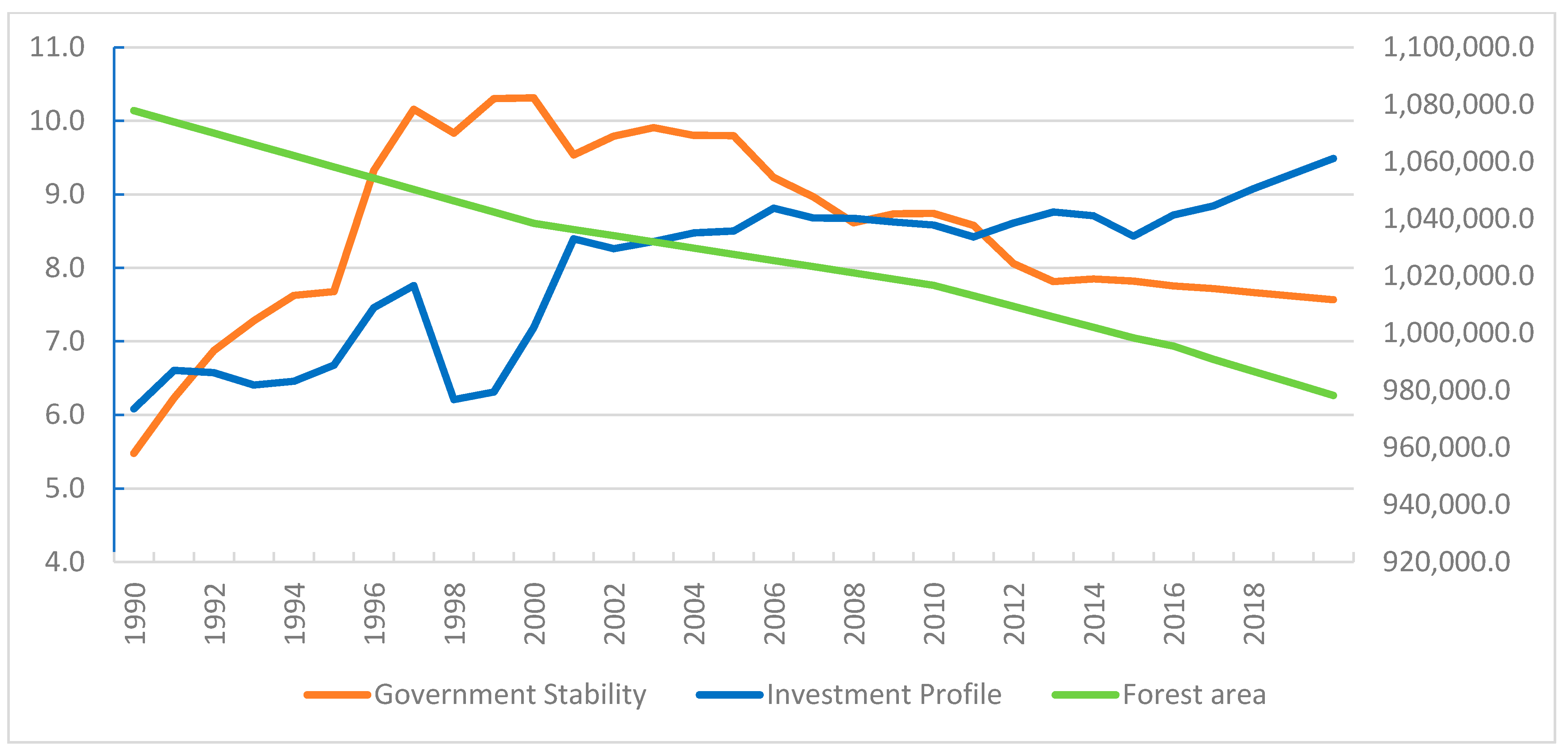
Figure 4 illustrates the dynamics of the evolution of forest cover, government stability, and investment profile in the countries of the ASEAN region. A relevant aspect is that forest cover has a decreasing trend during the analyzed period when forest cover has remained globally stable in recent years. The variables of stability of the government and the investment profile show fluctuations with upward and downward trends between 1990 and 2020. Government stability, in orange, indicates an increase in its values until 1997 to subsequently decrease due to lack of transparency, low coordination, and political problems of the countries. The investment profile has values lower than government stability, and as of 1999, this variable rises in low amounts until 2020. Thus, the problem of the decrease in vegetation cover is evident, and great efforts are required to mitigate its effects on the ecosystems. On the contrary, on average, the stability of the government and the investment profile has an increasing trend until the end of the 1990s. Both variables show a sustained decrease for approximately a decade from that period, whose trend has changed in recent years.

The excessive use of ecosystem resources leads to the collapse of protected areas, defined as the set of natural and human systems that offer people goods and services. However, it was found that the institutional framework in the local communities of Vietnam is divergent, generating more significant problems in the governance of protected areas [80]. Countries with a strong inflow of foreign capital are often associated with poor environmental regulation to maximize production. Hence, the importance of the creation and conservation of protected natural areas to conserve forests as a mechanism of environmental sustainability.

4. Econometric Strategy

Institutions are one of the mechanisms for applying long-term pro-environmental policies that promote environmental sustainability. The research seeks to assess the impact of government stability and investment profile on forest cover in the ASEAN region. A series of econometric methods are used to examine the causal link between the series to get the proposed objective. The incorporation of cross-sectional and temporal information facilitates understanding of the behavior of various units (N) over time (T). However, N and T differ in size because there are panels where T is less than N [81]. Several investigations have included homogeneity in the coefficients when this should not be valid for relatively large N and T [82]. Therefore, in our study, we applied the Pesaran and Yamagata test [20], which also considers the presence of cross-section dependence. This test raises the null hypothesis that there is homogeneity on the slope between the transverse units. Biased results are obtained when the homogeneous slope is included in the coefficients [83]. Although there are similarities between the ASEAN countries, factors may differentiate the countries from each other in aspects related to the variables analyzed.

In parallel, the dependency between the cross-sections determines the type of models to be used in the econometric estimates of panel data [84,85]. Likewise, Chudik and Pesaran [86] point out that the spatial effects, such as the countries’ economic networks, are part of the existence of transversal dependence. The cross-section dependence test is a diagnostic test for choosing between first or second-generation cointegration models [87]. We verify the dependence on the cross-sections using Pesaran’s CD test [88], stated in Equation (1). The CD test generates robust estimators without residual normality and structural shocks in the series [89]. The results of the Pesaran test [88] are contrasted with the test of Bailey et al. [90], to establish the factor strength of the estimates with greater precision.

$$CD=\left[\frac{2T}{N\left(N-1\right)}\left({\displaystyle \sum }_{i=1}^{N-1}{\displaystyle \sum }_{j=i+1}^N\widehat{p}ij\right)\right]$$

(1)

The presence of cross-sectional dependence in the panel requires the use of the second-generation unit root tests of Herwartz and Siedenburg [21], Pesaran [22], and Breitung [23] to know the behavior of the variables over time. In the same way, Westerlund’s second-generation cointegration test [91] is applied, which considers cross-sectional dependence and heterogeneity in the slope presented in Equation (2).

$$Y_{i,t}={\delta }_i{d}_t+{\alpha }_i\left(y_{i,t-1}-{\beta }_i{X}_{i,t-1}\right)+{\displaystyle \sum }_{j=1}^{Pi}{\alpha }_{ij{Y}_{it-j}}+{\displaystyle \sum }_{j=-qi}^{pi}{y}_{ij}{X}_{it-j}+{\epsilon }_{i,t}$$

(2)

where, d_t symbolizes the deterministic component of the model that can adopt values of $d_t=0$, $d_t=1$ and y $d_t=1-t$. Advance or delay orders are represented by pi and qi. The independent variables are denoted by $X_{it}$, and the error term is also included. Cointegration vectors are verified with the Westerlund test [92] in some panels and at the level of the entire panel with two variations with or without trend. To check the short- and long-run elasticities, we use recent estimators such as AMG, developed by Eberhardt and Bond [93] and Eberhardt and Teal [82], and the CCE-MG by Pesaran [22] and updated by Kapetanios et al. [94]. The common factor of both estimators considers the cross dependency and the heterogeneity of the parameters. The difference between both estimators is the common factor approximation method [89]. The advantage of these estimators is that they have heterogeneous properties and include the cross-sectional dependence of the variables [87]. In Equation (3), the approach of the AMG estimator is detailed, and in Equation (4), the formalization of the approach of the CCE-MG estimator. In addition, the CCE-MG estimator includes the average of the independent variables and the dependent variable indicated by $\overline{x}$ and $\overline{y}$.

$$AMG={\alpha }_i+B_i\Delta x_{it}+{\phi }_i{f}_t+{\displaystyle \sum }_{t=2}^T{X}_t+{\epsilon }_{it}$$

(3)

$$CCE-M{G}_{it}={\alpha }_i+B_i{x}_{it}+{\theta }_i{\overline{y}}_{it}+{\delta }_i{\overline{x}}_{it}+{\phi }_i{f}_t+{\epsilon }_{it}$$

(4)

In order to determine the elasticity and equilibrium, we use FMOLS in the long-run and complement it with dynamic ordinary least squares (DOLS). Additionally, to verify the significance of the coefficients in the short and long term, the technique proposed by Pesaran and Smith [83] of augmented autoregressive distributed delay modeling in cross-section (CS-ARDL) is used. This methodology was modified by Chudik et al. [94] in the presence of cross-section dependence and the heterogeneous slope. Its formalization is presented in Equation (5), where p and q are the numbers of lags, and the terms $\overline{x }$ and $\overline{y }$ are the number of lagged cross-sectional averages.

$$Y_{it}={\beta }_i+{\displaystyle \sum }_{k=1}^p{\theta }_{ik}{Y}_{it-k}+{\displaystyle \sum }_{k=0}^q{\delta }_{ik}{X}_{it-k}+{\displaystyle \sum }_{k=0}^{S\overline{x}\overline{y}}{\vartheta }_{ik}{\overline{Y}}_{t-k}{\overline{X}}_{t-k}+{\epsilon }_{it}$$

(5)

The econometric strategy is designed to verify the hypotheses and achieve the research objective.

5. Results and Discussion

Before the cointegration phase, the Pesaran and Yamagata slope homogeneity test is performed [20]. The null hypothesis that the coefficients were homogeneous is verified. The results in

Table 4. Results from Pesaran and Yamagata’s homogeneity test.

Tests	Delta	p-Values
$-\Delta$	15.08 ***	<0.0001
$-\Delta$adj	16.15 ***	<0.0001

H0: slope coefficients are homogenous and *** denote significance level at 0.1%.

indicate that both −∆ and $\Delta$_adj statistics are significant at 1%, which allows for rejecting the null hypothesis.

$-$$-$

Table 5. Results of cross-section dependence test.

Variables	Pesaran (2015)		Bailey, Kapetanios and Pesaran (2016)
	Statistics	p-Value	Statistics	p-Value
Forest area	−1.21 ***	<0.0001	29.46 ***	<0.0001
Government stability	12.49 ***	<0.0001	28.66 ***	<0.0001
Investment profile	10.28 ***	<0.0001	28.06 ***	<0.0001

Note: *** Denote significance level at 0.1%.

shows the results of the cross-section dependency test used to identify the unit root tests to be used in the cointegration approach. Two tests are used for a broad contrast of the results: the Pesaran [88] and the Bailey et al. [90] tests. Both tests indicate that the series has a dependency on the cross-sections, with a significance level of 1%. These diagnostic tests contribute to obtaining consistent estimators that give greater robustness to the model.

The results of the tests presented in Table 4 and Table 5 suggest the application of second-generation unit root tests. In this sense, the Herwartz and Siedenburg [21], Pesaran [22] and Breitung [23] tests are used. The series presents a trending behavior in the analysis period between 1990 and 2020. When the variables have an order of integration I (2), the trend component is lost and becomes a statistically significant stationary series.

Table 6. Results of second-generation unit root tests.

	Levels			Second Difference
	Herwartz and Siedenburg (2008)	Pesaran (2006)	Breitung (2000)	Herwartz and Siedenburg (2008)	Pesaran (2006)	Breitung (2000)
Forest area	−0.28	−0.95	−0.53	−1.97 ***	−5.75 ***	−7.24 ***
Government stability	−1.10	−2.02	−1.44	−3.39 ***	−6.18 ***	−5.05 ***
Investment profile	−0.82	−1.76	−0.46	−2.48 ***	−6.11 ***	−6.18 ***

Note: *** denotes statistical significance at 0.1%.

reports the results of the unit root tests applied to the series.

Table 7. Results of the Westerlund cointegration test (2007).

Statistic	Value	Z-Value	p-Value	Robust p-Value
Gt	−3.03 **	−1.69	0.04	0.11
Ga	−12.30	0.51	0.69	0.10
Pt	−8.63 ***	−2.39	0.00	0.05
Pa	−11.34	−0.35	0.36	0.14

Note: *** and ** denotes statistical significance at 0.1%, and 1%, respectively.

shows the results of Westerlund’s second-generation cointegration test [91], which tests the relationship between the variables in the presence of cross-sectional dependence. Cointegration statistics, at the group level and for the entire panel, are reported. The Gt and Ga statistics test has at least one unit in the panel that is cointegrated. Instead, Pt and Pk are the statistics that verify the cointegration of the panel as a whole. The statistics reveal that the forest area, government stability, and investment profile, which is a proxy for institutionality, are cointegrated in the short term. In other words, the variations generated in government stability and the investment profile cause immediate changes in the forest area. Positive results are achieved when governments efficiently manage public resources on environmental issues. In addition, with a higher investment profile, the country’s socio-economic conditions are improved. At the same time, this scenario gives rise to a greater institutionality that is rewarded in implementing policies that benefit the community in general.

Additionally, in

Table 8. Results of the Westerlund (2005) cointegration test.

Variance Ratio	Without Cross-Sectional Averages				With Cross-Sectional Averages
	Without Time Trend		With Time Trend		Without Time Trend		With Time Trend
Test some panels	Statistic	p-value	Statistic	p-value	Statistic	p-value	Statistic	p-value
	−2.69 ***	0.00	−3.28 ***	0.00	−2.74 ***	0.00	−3.37 ***	0.00
Test all panels	Statistic	p-value	Statistic	p-value	Statistic	p-value	Statistic	p-value
	−2.03 *	0.00	−2.71 ***	0.00	−2.01 ***	0.00	−2.66 ***	0.00

Note: *** and * denotes statistical significance at 0.1%, and 5%, respectively.

, the Westerlund cointegration results [92] are reported. This test indicates the cointegration of some panels or the entire panel considering two measurements. In the first part, the results are reported without considering the average cross-sectional dependence, and in the second part, the cross-sectional dependence is incorporated. Both sections detail the statistics with and without trends. Based on the significance level, the presence of cointegration is revealed in the entire panel of variables included in the study. This fact means that there is a cointegration vector linking them over time. Following Hao et al. [60], when seeking sustainable economic growth balanced with the environment, conservation of forest resources is achieved, thus avoiding environmental degradation. The quality of human life is improved when the preservation of the land becomes a priority situation to support ecosystem services in critical conditions [63]. In this sense, the development of institutions constitutes a critical point so that, through rigid regulations, it contributes to the reduction of productive pollution due to economic activity [66].

Table 9. Short-run elasticity.

	Panel AMG	Panel CCE-MG
Government stability	−0.001	−0.003
	(−0.07)	(−0.32)
Investment profile	−0.003	−0.01
	(−1.56)	(−0.48)
c_d_p		3.05 ***
		(3.98)
Forest area _avg	2.98 ***
	(3.94)
Government stability avg	0.003
	(0.22)
Investment profile _avg	0.002
	(1.30)
Constant	−0.002	−0.003
	(−0.27)	(−0.49)
Observations	29	29
Countries (N)	8	8
Chi-squared	0.32	0.34

Note: *** denotes statistical significance at 0.1%.

reports the short-term elasticity using two estimators: AMG and CCE-MG for the panel. Both estimators indicate no statistical significance in any of the variables. In the lower part, the elasticities are shown considering the average of the cross-sections represented by the suffix avg next to each variable. This denotation shows the average coefficients with cross-sectional dependence applied to the dependent variable and the explanatory variables. In other words, we show that the average effect of vegetation cover is significant in the short term in the countries of the ASEAN region. Similarly, the CCE-MG estimator includes the term c_d_p which symbolizes the common dynamic process that analyzes the common time-varying effect of all cross-sectional data. The behavior of this relationship is justified because, in many cases, the policies that governments implement are not carried out efficiently. The absence of statistical significance in the relationship is supported by the countries’ low institutional quality which prevents achieving a sustainable environment for present and future generations [67]. Likewise, the lack of investment in environmental technology is another problem that countries present, which causes more significant pollution to be generated. In developed economies, institutionality has been improving along with more significant innovation and sustainable environmental policies that have resulted in reducing environmental degradation [68]. In turn, Ali et al. [72] emphasized that quality institutions are indispensable to improving environmental quality.

To check the long-term relationship, we use FMOLS and DOLS in the global panel. The results in

Table 10. Long-run elasticity estimates from panel FMOLS and DOLS.

	Panel-FMOLS		Panel-DOLS
	Coefficient	t-Statistic	Coefficient	t-Statistic
Government stability	0.00	−0.14	0.00	1.83
Investment profile	0.00	0.40	0.00	1.66

establish the absence of long-term equilibrium between government stability, investment profile, and forest area. Most countries are susceptible to political instability, high corruption, weak institutions, and environmental stress caused by the excessive use of energy based on fossil fuels and traditional technology that affect natural resources [61]. This is why good governance is required, to reduce the threats caused by persistent deforestation in various areas, threatening livelihoods that depend on forests [73]. In addition, it is necessary that, in the long term, new environmental planning is formulated that focuses on a new forest management design that incorporates efficient sectoral policies [75].

Table 11. Long-run elasticity estimates from country FMOLS.

	Government Stability	t-Statistics	Investment Profile	t-Statistics
Brunei Darussalam	−0.00	−0.20	−0.00	0.29
Indonesia	−0.00 *	−2.10	0.00 *	2.89
Malaysia	−0.00 ***	−7.02	0.00	0.77
Myanmar	0.00 *	2.00	−0.00	−0.41
Philippines	−0.00	−0.04	0.00	0.11
Singapore	0.00 *	2.57	0.00	0.29
Thailand	−0.00	−1.36	−0.00 *	−2.68
Vietnam	0.00	0.79	−0.00	−1.25

Note: *** and * denotes statistical significance at 0.1%, and 5%, respectively.

reports the long-term cointegration results by ASEAN member countries. It is confirmed that most of the panels do not have statistical significance in the variables. However, Indonesia, Malaysia, Burma, and Singapore are highlighted as the economies that reflect a statistically significant relationship between government stability and forest area in the long term. Although, in Indonesia and Malaysia, the existing link is negative, and positive for Burma and Singapore. Similarly, it is confirmed that the investment profile maintains a positive relationship with the forest area in Indonesia and a negative relationship with Thailand.

Finally, the estimation to determine the significance of the coefficients in the short and long term uses the CS-ARDL. There is no statistical significance for any variable in the short term, unlike in the long term, where only government stability is positive and significant in the forest area in the ASEAN countries. In the long term, the significance of government stability is supported by the existing synergy between institutions, governmental and non-governmental organizations, and multiple social agents for the proposal of ideas that design programs for the restoration and protection of shared resources [74]. Thus, institutions should try to regulate their activities in the short and long term to avoid affecting ecosystems [52]. It is also essential to spread greater environmental awareness in environmental conservation, especially in fragile and limited ecosystems [50].

Furthermore, the results in

Table 12. Long-run and short-run estimations using CS-ARDL.

	Short-Run Coefficients	Long-Run Coefficients
Government stability	0.002	0.99 ***
	(0.40)	(1992.72)
Investment profile	−0.001	−0.001
	(−0.15)	(−0.15)

Note: *** denotes statistical significance at 0.1%, and the t value are in parentheses.

show that the impact of government stability on forest cover is more significant in the long-run than in the short-run estimations. This fact suggests that political stability can have a more significant influence if pro-environmental actions are stable over time.

6. Conclusions and Policy Implications

The conservation of forests is imperative in achieving the population’s quality of life because it purifies the air and water. The conservation of natural areas in the ASEAN region is relevant for the member countries of the ASEAN region. Over time, a series of policies and measures have been implemented to promote the conservation of plant cover. This research examined the impact of government stability and investment profile on forest cover in countries in the ASEAN region. The case study is relevant because it is one of the regions where forest cover has decreased in recent decades. This fact raises the urgent need to implement institutional policies to conserve forests in their natural state. In addition, we highlight the relevance of the creation and maintenance of protected natural areas to ensure the sustainability of future generations in these countries.

In general, the results considered the dependency in cross-sections and the heterogeneity on the slope. The existence of dependence between the panels supports the elaboration and application of common pro-environmental policies among the countries within the ASEAN region. However, it is relevant to consider the characteristics that distinguish them from the countries analyzed. We find a long-run relationship between the series, indicating that the impact of government stability and investment profile has an equilibrium relationship with forest cover. This finding implies that the covariates can be used as a pro-environmental policy instrument to reduce deforestation in the countries analyzed.

The region must contemplate, with concern, the productive aspects of forest resources and the conservation of the environment. Therefore, implementing a comprehensive forest policy must recognize forests’ economic, ecological, and social functions and their products. A comprehensive approach implies that forestry (and development) policies are oriented to a new, more complementary, and participatory vision, which combines productive activities, human beings, and natural resources. Moreover, it is necessary to emphasize the participation of local governments since they have critical responsibilities in forest management. Furthermore, as recognized political authorities, they can undertake many initiatives to impact the forestry sphere.

Future research could increase the number of institutional variables as explanatory factors of forest cover dynamics in a context of strong economic and financial globalization. Environmental sustainability requires efforts, by the government and society in general, to ensure the well-being of future generations.