Detection of Multiple Drones in a Time-Varying Scenario Using Acoustic Signals

Abstract

Detection of unauthorized drones is mandatory for defense organizations and also for human life protection. Currently, detection methods based on thermal, video, radio frequency (RF) and acoustic signals exist. In previous research, we presented an acoustic signals-based multiple drones detection technique utilizing independent component analysis (ICA) in the presence of interfering sources. In this paper, a method is proposed in which the mixed signals are first separated taking the ICA technique into account. After extracting the features, the support vector machines (SVM) and the k-nearest neighbors (KNN) are used to identify multiple drones in the field. This technique can detect multiple drones in static and quasi-static mixing scenarios, while failing in time-varying scenarios. In this paper, a time-varying drone detection technique (TVDDT) is proposed that first stores a data set of the mixed signals in a time-varying scenario, where time variations occur within the processing data blocks. After estimating the mixing matrices, we developed a technique to track variations in the channel. This technique is based on variations in the mixing coefficients. The proposed channel tracking technique performs classification and detection based on minimum variation criteria in the channel. The proposed TVDDT technique is evaluated through simulations and its superior performance is observed.

1. Introduction

Today’s modern drones consist of advanced telecommunication, electronics and control technologies, having uncountable uses in many fields such as remote sensing [1], navigation [2,3,4], archaeology [5,6], journalism [7], the environment [8,9] and agriculture [10]. Furthermore, in [11], the authors presented point-to-point architecture for a single drone detection. In [12], drone detection based on cognitive internet of things was performed. Image processing was utilized for drone detection in [13]. Different machine learning algorithms were utilized in [14,15,16] for the detection of unauthorized drones. In [17], a radio frequency (RF)-based detection was presented. Drone detection based on radio access networks was carried out in [18]. Sound-based drone detection was performed in [19,20,21,22]. Indoor detection of unauthorized drones was performed in [23,24,25].

The unauthorized movement of drones can motivate illegal activities that may cause security threats to an organization or country [26,27,28]. Thus, the detection of unauthorized drones is necessary. Furthermore, drone detection methods based on sound, radio frequency (RF) signal, image processing, radar technology and video signals are presented in [11,12,14,29,30,31,32,33,34,35,36,37,38,39]. The RF-signals-based technique fails in unfavorable atmospheres and also fails to identify mini drones. Similarly, the image- and video-based methods require high-performance cameras and computationally efficient circuitry; they are hence very expensive solutions. Moreover, the image- and video-based techniques also have shortcomings of fixed orientation. Acoustic-signal-based identification is cost effective and practically applicable, but the presence of interfering sources make it more complex. The audio-based drone detection methods presented in [14,20,21,22] consider the drone and the interference ring sources independently without considering practical scenarios. In practical scenarios, the recorded signals are mixtures of the source signals, including the drone sound as well as the interfering sources. All these papers also considered single drone detection at a time in the sensing field. Moreover, in [30], the authors proposed a multiple-drones detection technique based on independent component analysis (ICA). In [30], multiple drones and interfering sources are considered while the channel is kept quasi-static. The technique presented in [30] is practically applicable and works well in the case of static or quasi-static channels. In quasi-static channels, the mixing matrix remains constant during the processing data block. In practical scenarios, the drones and the interfering sources are not static, which causes failure of the quasi-static condition. This becomes a challenging issue for the ICA algorithms to blindly unmix the mixed data in time-varying mixing scenarios. In fact, the role of the ICA algorithm is to estimate the mixing coefficients of the mixing system. In this case, if the mixing coefficients change within the processing data block, the ICA algorithm fails to estimate these coefficients properly.

This work presents a time-varying drone detection technique (TVDDT) to detect single and multiple drones in a sensing field in a time-varying scenario. The role of the ICA algorithm is to unmix the mixed audio signals. If there are multiple drones in the field, the ICA algorithm can easily unmix them without any modification in the algorithm. The proposed technique is based on audio signals processing. The drone detection is performed considering the strong interfering sources. These sources include sounds of birds, rain, air, airplanes, etc. The drone detection is performed considering all the drones and interfering sources in motion. The proposed TVDDT technique first stores a long data set simulated through multiple microphones. The mixed data are converted to smaller data blocks for unmixing using the ICA algorithm and classification. Once the signals are unmixed, the classification technique can classify the signals into drone and non-drone signals even if there are multiple drones in the sensing field. Moreover, conversion into smaller data blocks make it possible to detect variations in the channel. Rapid variations in the channel produce low-quality results. The unmixing is performed over smaller data blocks while observing the channel variations through a technique proposed for tracking the channel variations. This is an iterative technique that compares the mixing coefficients obtained from the data set with the other data set, and observes the variations. These variations depend on the drone speed; large variations are observed at a high speed of the drone and vice versa. These variations are recorded for various data blocks and the results are analyzed for small variations in the channel. In case of small variations, a better unmixing performance is observed. Furthermore, the linear predictive cepstral coefficients (LPCC) and mel-frequency cepstral coefficients (MFCC) [40] are utilized for feature extraction. Afterwards, the support vector machine (SVM) [41] is utilized for classification of the extracted features once better unmixing performance is obtained. The key contributions of this research are as follows:

• Drone detection has been performed in previous works while considering the quasi-static channels. In this research, we concentrate on time-varying mixing channels to detect the unauthorized drones in a practical scenario. In order to achieve this objective, a channel tracking technique is proposed to track the channel variations in a time-varying scenario. The proposed technique is based on the estimated mixing matrices using the FastICA algorithm [42].
• The time varying drone detection (TVDDT) technique is proposed to detect single as well as multiple drones in the presence of strong interfering sources considering the time-varying scenario in which the drones are in motion.
• The detection of the drones is performed in a time-varying scenario considering the drones when the interfering sources are in motion. This becomes a challenging issue in drone detection utilizing audio signals.

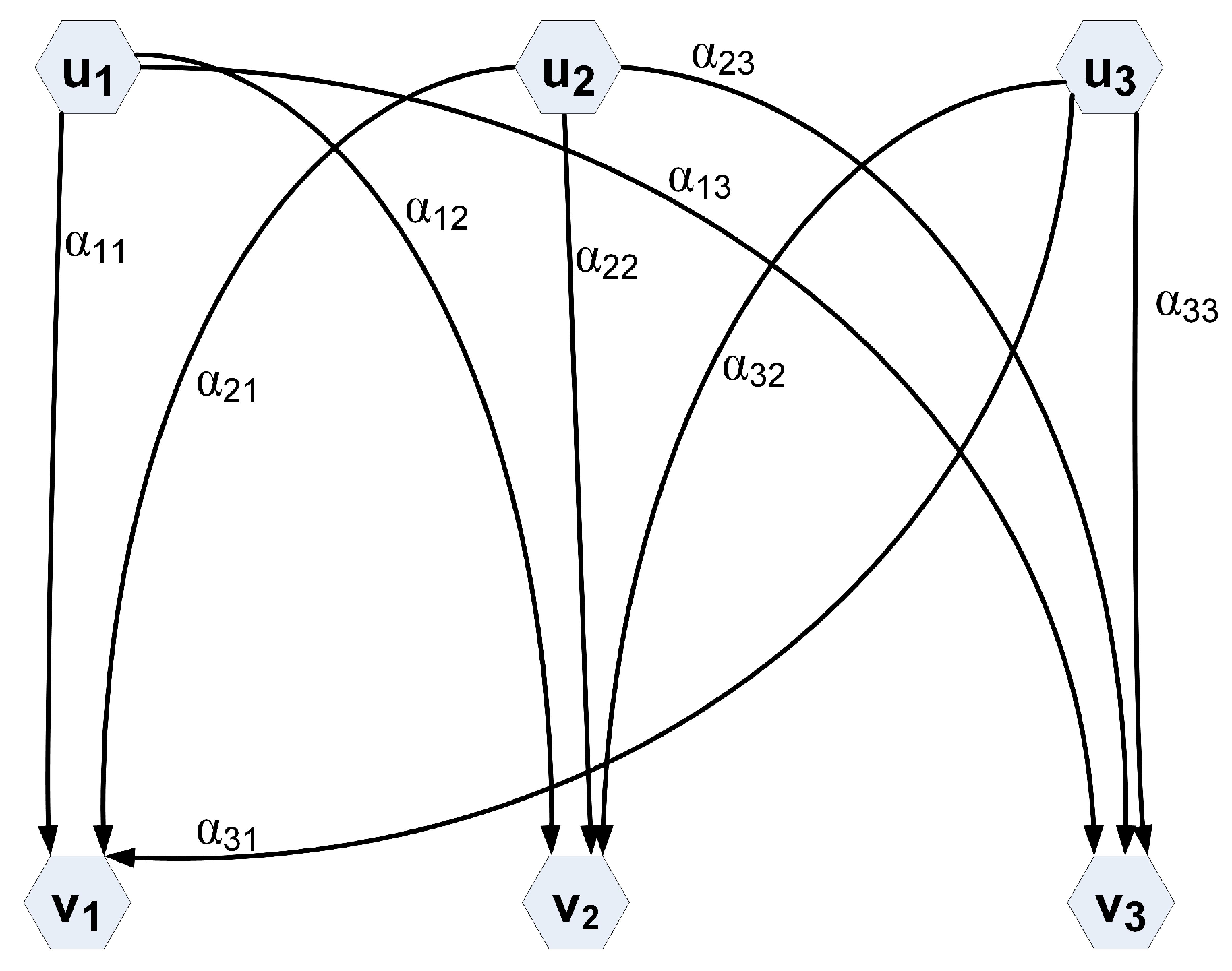
The rest of the paper is organized as follows. Section 2 presents the system model of the proposed algorithm. The proposed TVDDT technique and the time-varying scenario of the flying drones is explained in Section 3. Simulation results and the conclusion are provided in Section 4 and Section 5, respectively. Moreover, lowercase letters are used for scalars, lowercase boldface letters for vectors and uppercase boldface letters for matrices. Transpose is denoted by uppercase superscript T. A list of abbreviations is also included in

Table 1. List of abbreviations.

ICA	Independent component analysis
Radio frequency	RF
Support vector machines	SVM
SNR	Signal-to-noise ratio
$SIR$	Signal-to-interference ratio
K-nearest neighbors	KNN
Time-varying drone detection technique	TVDDT
Linear predictive cepstral coefficients	LPCC
Mel-frequency cepstral coefficients	MFCC
Power spectral density	PSD

for the clear understanding of the reader.

2. The System Model

This section presents the drones and the interfering signals in the independent component analysis (ICA) data model. The application scenario is given in Figure 1. This figure demonstrates the practical scenario of the drone and the interfering sources. Although we utilized data downloaded from a standard database rather than the hardware implementation, this figure makes it easy for the reader to clearly understand the application scenario. Furthermore, N number of acoustic sources ${\mathbf{u}}_1,{\mathbf{u}}_2,\dots ,{\mathbf{u}}_N$ were considered, as shown in Figure 2 with N = 8. All these signals were downloaded from the standard databases usually utilized for research and which are freely available at [43]. These sound signals were downloaded in a WAV format having a sampling frequency of 96 kHz and a 24 bit resolution. In order to clearly understand the system model of the proposed technique, we considered Figure 2, which consists of N number of sensors. The source signals were downloaded from a standard database having block length L as ${\mathbf{u}}_n=[u_{n1},u_{n2},\dots ,u_{nL}]$, with $n=1,2,\dots ,N$. The downloaded source signals were mixed using MATLAB code with random mixing matrices. The mixed signals were linear mixtures of all the sources as ${\mathbf{v}}_1,{\mathbf{v}}_2,\dots ,{\mathbf{v}}_N$. Furthermore, the sensors in Figure 2 show how mixing occurs in the practical scenario. After mixing, the mixed data is processed using the independent component analysis (ICA) algorithm for unmixing, as shown in Figure 2. The unmixed signals are ${\mathbf{y}}_1,{\mathbf{y}}_2,\dots ,{\mathbf{y}}_N$. The mixture signals can be modeled mathematically as:

$$\mathbf{V}=\mathbf{A}\mathbf{U}+\mathbf{X}$$

(1)

The $\mathbf{V}$ represents the $N\times L$ mixed data matrix, $\mathbf{A}$ is the $N\times N$ mixing matrix, $\mathbf{U}$ is the $N\times L$ source data matrix and $\mathbf{X}$ represents the atmospheric acoustic noise. The square mixing matrix was considered because the ICA algorithm requires an equal number of the source and the mixture signals. Equation (1) represents the quasi-static mixing scenario in which the mixing matrix remains constant during the processing data block. Various mixing models were used in the ICA signal processing, such as constant mixing, quasi-stationary mixing, ill-conditioned mixing, instantaneous mixing, convolutive mixing, time-varying mixing, non-linear mixing and under and over-complete mixing [44]. Time-varying mixing values of the mixing matrix varied during the processing data block. The mixing matrix varied during the processing data block; the mixing matrix can be modeled as follows:

$$\mathbf{V}=\mathbf{A}\mathbf{U}+\Delta \mathbf{U}+\mathbf{X}$$

(2)

The $\Delta \mathbf{U}$ is the error signal, and the goal is to compensate this parameter in the ICA signal processing. The new mixing matrix ${\mathbf{A}}^{\prime }$ can be written as:

$$\mathbf{A}{}^{\prime }=\mathbf{A}+\Delta$$

(3)

In the literature, it is assumed that the variations in the channel are slow, i.e., $\Delta =0$, or small data block lengths are assumed in order to neglect variations in the processing data blocks. The time-varying mixing in the processing data blocks becomes a challenging problem if the above two assumptions are false. Furthermore, after unmixing using the ICA, the estimated signals are represented as:

$$\mathbf{Y}=\mathbf{W}\mathbf{V}$$

(4)

The $\mathbf{W}$ is the inverse of $\mathbf{A}{}^{\prime }$ and is known as the unmixing matrix.

3. The Proposed TVDDT Technique

Detection of unauthorized drones is performed in the literature utilizing various techniques. These techniques include RF communication, acoustic measurement, as well as image and video signal processing techniques. However, the RF-based detection fails under severe atmospheric conditions and does not succeed in identifying small and variable-shape drones [11]. Similarly, the image- and video-based methods are computationally inefficient and require expansive circuitry; hence, these are very expensive solutions [11,30]. Sound-based detection is more practical, but various interfering sound sources such as birds, airplanes, wind, thunderstorms, etc., make it more challenging. We proposed an independent component analysis (ICA) technique in [30] to detect multiple drones in the presence of these interfering sources. In [30], it is assumed that the channel is quasi-static while in a practical scenario the detected drone is moving. Due to drone movement, the mixing matrix varies within the processing data block and the SVM technique fails to detect the drone sound. The technique proposed in this work is capable of detecting the unauthorized drones in a sensing field in a time-varying scenario. In the next subsection we explain the time-varying mixing scenario utilized in the development of the proposed technique.

3.1. Time-Varying Scenario of the Flying Drones

Consider Figure 3, where the drone is initially at a point P and the ground acoustic sensing unit is at a distance d. At this point, the sensing unit stores the sounds of a single drone or multiple drones and the attenuation depends on the distance d. With increased values of d, the signal amplitude decreases. At point P and distance d, the sensing mechanism of the drone sound is illustrated in Figure 4, where all $a_{ij}$ are the mixing coefficients for $i=1,2,3$ and $j=1,2,3$ because every sensor simulates the mixture of the drone sound. Moreover, let the drone move from point P to the new point, Q. Now, the distance changes from d to $d^{\prime }$ and the mixing coefficients change, as illustrated in Figure 5. In this figure, we consider an equal number of sources and sensors as three, and the new mixing coefficients in this figure are ${\alpha }_{ij}=a_{ij}+{\Delta }_{ij}$. The time-varying mixing coefficients are shown in Equation (5).

$$\mathbf{A}{}^{\prime }=\left[\begin{array}{cccc}{a}_{11}+{\Delta }_{11}& a_{12}+{\Delta }_{12}& \dots & a_{1L}+{\Delta }_{1L}\\ a_{21}+{\Delta }_{21}& a_{22}+{\Delta }_{22}& \dots & a_{2L}+{\Delta }_{2L}\\ ⋮& ⋮& \ddots & ⋮\\ a_{N1}+{\Delta }_{N1}& a_{N2}+{\Delta }_{N2}& \dots & a_{NL}+{\Delta }_{NL}\end{array}\right]$$

(5)

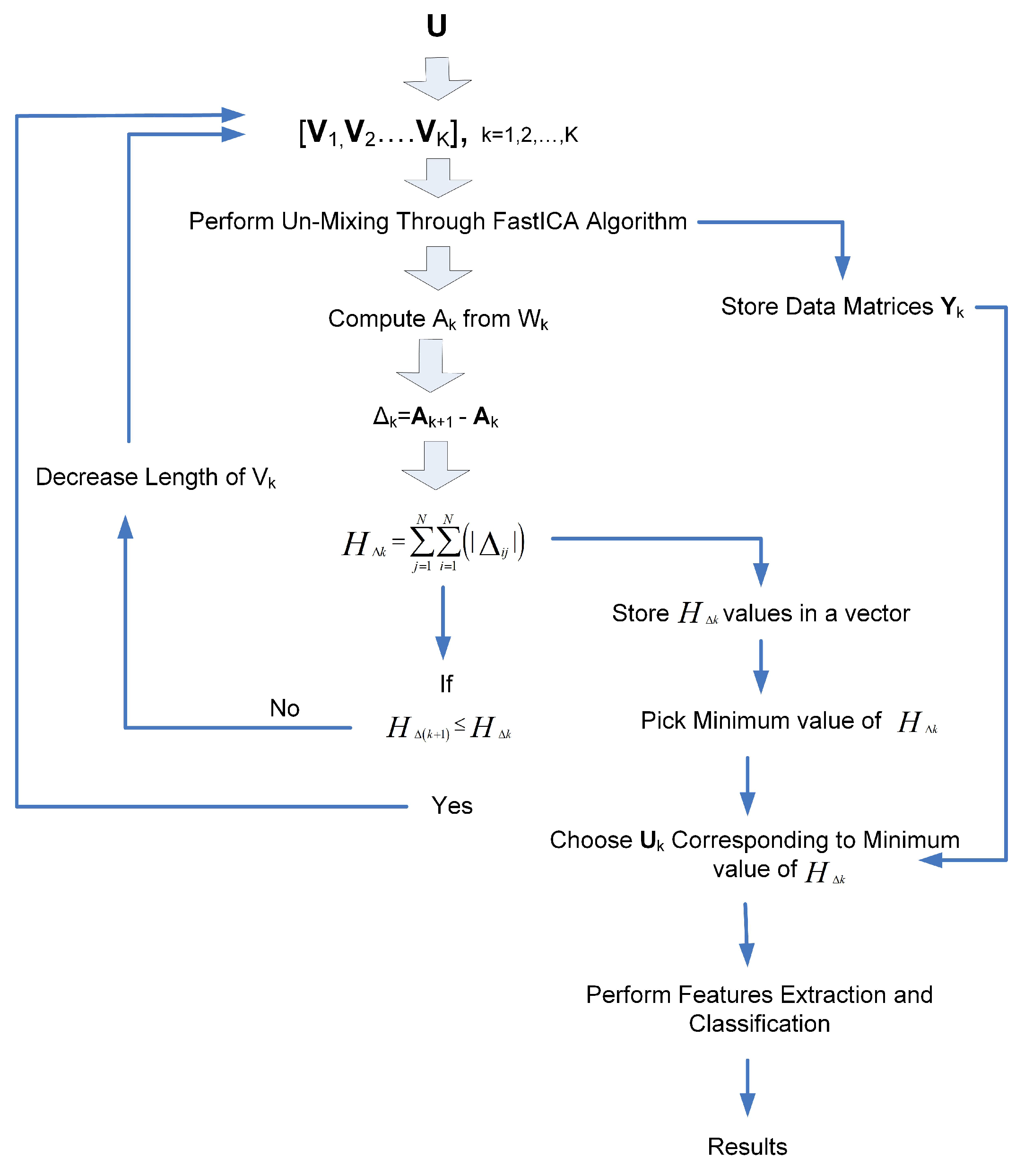
3.2. The TVDDT Technique

In time-varying scenario, the mixing coefficients are changing within the processing data blocks and the ICA algorithm is unable to track these variations. Once the unmixing is performed properly, the feature extraction and classification techniques work as shown in [30]. In this work, we proposed a time-varying drone detection technique (TVDDT) to detect single and multiple drones in a sensing field using acoustic signals. First, we downloaded a long data set of the acoustic signals of the drones and the interfering sources, as shown in Figure 3. The proposed technique tracks the channel variations due to either drone movement or interfering sources. A data flow diagram of the proposed TVDDT technique is given in Figure 6. The source data matrix $\mathbf{U}$ contains the drones and the interfering source signals. The mixture signals are ${\mathbf{V}}_1,{\mathbf{V}}_2,\dots ,{\mathbf{V}}_K$, where $k=1,2,\dots ,K$. After computing ${\mathbf{A}}_k$, ${\Delta }_k$ is computed as:

$${\Delta }_k={\mathbf{A}}_{k+1}-{\mathbf{A}}_k=\left[\begin{array}{cccc}{\Delta }_{11}& {\Delta }_{12}& \dots & {\Delta }_{1N}\\ {\Delta }_{21}& {\Delta }_{22}& \dots & {\Delta }_{2L}\\ ⋮& ⋮& \ddots & ⋮\\ {\Delta }_{N1}& {\Delta }_{N2}& \dots & {\Delta }_{NN}\end{array}\right]$$

(6)

Note that the ${\Delta }_k$ represents variations in the mixing matrix explained above. Once ${\Delta }_k$ is calculated, the $H_{\Delta k}$ is calculated as:

$$H_{\Delta k}=\sum _{i=1}^N\sum _{j=1}^N\left|{\Delta }_{ij}\right|$$

(7)

The $H_{\Delta k}$ is the measure for predicting variations in the channel. A high value of $H_{\Delta k}$ represents large variations in the channel and conversely. Finally, the following condition is checked:

$$H_{\Delta k+1}\le H_{\Delta k}$$

(8)

If the above condition is true, select another data set ${\mathbf{V}}_{k+1}$; if this fails, decrease the data block length and perform the separation again. Now, select the extracted results ${\mathbf{Y}}_k$ corresponding to the minimum value of $H_{\Delta k}$ for feature extraction and classification. The proposed technique is summarized step by step in Algorithm 1.

The power spectral density (PSD) values are calculated by passing the ICA unmixed data through octave band filtering [45]. The audio spectrum (20 Hz to 20 kHz) is divided into 11 bands according to Equation (9).

$$\begin{array}{c}\hfill f_7^c=1000 \mathrm{Hz}\\ \hfill f_{n-1}^c=0.5f_n^c\\ \hfill f_{n+1}^c=2f_n^c\end{array}$$

(9)

The $f_7^c$ represents the 7^th octave band central frequency, and $f_{n-1}^c$ and $f_{n+1}^c$ are the lower and upper central frequencies, respectively. Similarly, the upper and the lower frequencies for each central frequency are $f_n^l=\sqrt{2}{f}_n$ and $f_n^l=f_n/\sqrt{2}$. Initially, different octave bands are obtained from a signal and then the RMS and PSD of each band is computed. By using the computed feature vectors, the sounds are classified as drone and non-drone sounds through algorithms.

Algorithm 1: The TVDDT algorithm.

In another technique, we used the MFCC calculated from the PSD of the audio signal. PSD is calculated through the filter banks as given in Equation (10).

$$\begin{array}{c}\hfill \begin{array}{c}\hfill P_h\left(n\right)=\left\{\begin{array}{cc}0,\hfill & n<f(h-1)\hfill \\ \frac{n-f(h-1)}{f\left(h\right)-f(h-1)},\hfill & f(h-1)\le n\le f\left(h\right)\hfill \\ \frac{f(h+1)-n}{f(h+1)-f\left(h\right)},\hfill & f\left(h\right)\le n\le f(h+1)\hfill \\ 0,\hfill & n>f(h+1)\hfill \end{array}\right.\end{array}\end{array}$$

(10)

The h and f represent the number of filters and mel-spaced frequencies, respectively.

4. Simulation Results

The effectiveness of the proposed technique for the detection of multiple drones is evaluated in this section using audio signals and a time-varying scenario. It must be noted that Figure 1 demonstrates the practical scenario of the drone and the interfering sources. Although we utilized data downloaded from a standard database rather than the hardware implementation, this figure makes it easy for the reader to clearly understand the application scenario. Similarly, Figure 3 explains the behavior of the flying drone from a specific point to another point. This figure shows that the value of the mixing coefficient changes with the change in position of the drone. In addition, this statement is also true for the interfering sources if they move from one point to another point.

In [30], we addressed this issue for a quasi-static mixing condition in the presence of strong interfering sources. In a practical scenario, the detected drones and the interfering sources are moving and the resultant mixing coefficients are time-varying. These variations may be slow or fast depending on the speed of the drones and interfering sources. In fact, the signals are the mixtures of all the surrounding audio sources, such as drones, birds, wind, thunderstorm, airplanes, rain, etc. The time-domain versions of these interference signals along the drone signal are demonstrated in Figure 7. All these signals were downloaded from the standard databases usually utilized for research and which are freely available at [43]. These sound signals were downloaded in a WAV format having a sampling frequency of 96 kHz and a 24 bit resolution. The source signals ${\mathbf{u}}_1,{\mathbf{u}}_2,\dots ,{\mathbf{u}}_6$ were multiplied with a random mixing matrix $\mathbf{A}$ to obtain the desired mixed data. The multiplication of the source signals with the mixing matrix demonstrates the mixing mechanism of the multiple mixes. The mixing process is mathematically illustrated in Equation (11).

$$\left[\begin{array}{cccc}{v}_{11}& v_{12}& \dots & v_{1L}\\ v_{21}& v_{22}& \dots & v_{2L}\\ ⋮& ⋮& \ddots & ⋮\\ v_{61}& v_{62}& \dots & v_{6L}\end{array}\right]=\left[\begin{array}{cccc}{a}_{11}& a_{12}& \dots & a_{16}\\ a_{21}& a_{22}& \dots & a_{26}\\ ⋮& ⋮& \ddots & ⋮\\ a_{61}& a_{62}& \dots & a_{66}\end{array}\right]\left[\begin{array}{cccc}{u}_{11}& u_{12}& \dots & u_{1L}\\ u_{21}& u_{22}& \dots & u_{2L}\\ ⋮& ⋮& \ddots & ⋮\\ u_{61}& u_{62}& \dots & u_{6L}\end{array}\right]$$

(11)

The mixed signals obtained are shown in Figure 8 for a random mixing matrix of size $6\times 6$. Hence, the technique presented in [30] fails in practical scenarios.

A performance evaluation was carried out using a Monte Carlo simulation. All simulations were performed using MATLAB 9.0. Furthermore, the lengths of the mixed data blocks were utilized in simulation ranges from 1000 to 10,000 samples. The performance evaluation criterion used was signal-to-interference ratio ($SIR$) [30]. $SIR$ in dB of a single data block is written as follows:

$$SI{R}_{\left(\mathrm{dB}\right)}=10\log \left({\displaystyle \frac{1}{L}}\sum _{n=1}^L{\displaystyle \frac{\mathbf{u}{\left(n\right)}^2}{\mathbf{u}\left(n\right)-\mathbf{y}{\left(n\right)}^2}}\right)$$

(12)

A time-varying scenario was utilized in the simulations in which the mixing matrix varies during a single data set. We utilized the source signals of Figure 7. The resultant mixing matrix is shown in Equation (13) with six source signals. Initially, the increasing values of $H_{\Delta k}$ were considered as varying from 0 to 2.9, where $H_{\Delta k}$ could be observed from Equation (7). The increasing value of $H_{\Delta k}$ means that the source signals were moving away from the sensing unit. The simulations were performed and the $H_{\Delta k}$ values are demonstrated in Figure 9. We also considered that some of the sources were moving away and some moving towards the sensing unit. The results are given in matrix form in Equation (14), where the $H_{\Delta k}$ values initially decreased from $1.4809$ to $0.0117$ and then increased up to $1.1224$. These results are also given in Figure 10, where the $H_{\Delta k}$ variations can be observed clearly. Furthermore, the randomly moving sources are considered next and the results are illustrated in Figure 11. It can be clearly observed from the figure that the $H_{\Delta k}$ values varied between $h_2=0.064$ and $h_1=0.102$. These results are also demonstrated in Equation (15), where values of $h_1$ and $h_2$ are highlighted in red color. It must be noted that J represents the number of experiments performed.

$${\mathbf{A}}^{\prime }=\left[\begin{array}{cccccc}{a}_{11}+{\Delta }_{11}& a_{12}+{\Delta }_{12}& a_{13}+{\Delta }_{13}& a_{14}+{\Delta }_{14}& a_{15}+{\Delta }_{15}& a_{16}+{\Delta }_{16}\\ a_{21}+{\Delta }_{21}& a_{22}+{\Delta }_{22}& a_{23}+{\Delta }_{23}& a_{24}+{\Delta }_{24}& a_{25}+{\Delta }_{25}& a_{26}+{\Delta }_{26}\\ a_{31}+{\Delta }_{31}& a_{32}+{\Delta }_{32}& a_{33}+{\Delta }_{33}& a_{34}+{\Delta }_{34}& a_{35}+{\Delta }_{35}& a_{36}+{\Delta }_{36}\\ a_{41}+{\Delta }_{41}& a_{42}+{\Delta }_{42}& a_{43}+{\Delta }_{43}& a_{44}+{\Delta }_{44}& a_{45}+{\Delta }_{45}& a_{46}+{\Delta }_{46}\\ a_{51}+{\Delta }_{51}& a_{52}+{\Delta }_{52}& a_{53}+{\Delta }_{53}& a_{54}+{\Delta }_{54}& a_{55}+{\Delta }_{55}& a_{56}+{\Delta }_{56}\\ a_{61}+{\Delta }_{61}& a_{62}+{\Delta }_{62}& a_{63}+{\Delta }_{63}& a_{64}+{\Delta }_{64}& a_{65}+{\Delta }_{65}& a_{66}+{\Delta }_{66}\end{array}\right]$$

(13)

$${\mathbf{H}}_{\Delta k}=\left[\begin{array}{cccccccccc}1.4809& 1.4541& 1.4273& 1.4005& 1.3737& 1.3470& 1.3202& 1.2934& 1.2667& 1.2399\\ 1.2131& 1.1864& 1.1596& 1.1329& 1.1061& 1.0794& 1.0526& 1.0259& 0.9992& 0.9724\\ 0.9457& 0.9190& 0.8923& 0.8656& 0.8389& 0.8122& 0.7855& 0.7588& 0.7321& 0.7055\\ 0.6788& 0.6521& 0.6255& 0.5988& 0.5722& 0.5456& 0.5189& 0.4923& 0.4657& 0.4391\\ 0.4125& 0.3859& 0.3593& 0.3328& 0.3062& 0.2796& 0.2531& 0.2266& 0.2000& 0.1735\\ 0.1470& 0.1205& 0.0941& 0.0676& 0.0411& 0.0147& 0.0117& 0.0382& 0.0646& 0.0910\\ 0.1173& 0.1437& 0.1700& 0.1963& 0.2226& 0.2489& 0.2752& 0.3014& 0.3277& 0.3539\\ 0.3801& 0.4062& 0.4324& 0.4585& 0.4845& 0.5106& 0.5366& 0.5626& 0.5886& 0.6145\\ 0.6404& 0.6662& 0.6921& 0.7178& 0.7436& 0.7693& 0.7949& 0.8205& 0.8460& 0.8715\\ 0.8969& 0.9223& 0.9476& 0.9728& 0.9980& 1.0230& 1.0480& 1.0729& 1.0977& 1.1224\end{array}\right]$$

(14)

$${\mathbf{H}}_{\Delta k}=\left[\begin{array}{cccccccccc}0.0805& 0.0836& 0.0887& 0.0755& 0.0808& 0.0893& 0.0817& 0.0921& 0.0860& 0.0948\\ 0.0931& 0.0950& 0.0904& 0.0866& 0.0901& 0.0921& 0.0923& 0.0728& 0.0832& 0.0891\\ 0.0907& 0.1008& 0.0790& 0.0867& 0.1009& 0.0927& 0.0765& 0.0837& 0.0874& 0.0855\\ 0.0962& 0.0815& 0.0908& 0.0891& 0.0811& 0.0864& 0.0753& 0.0805& 0.0949& 0.0975\\ 0.0923& 0.0879& 0.0938& 0.0823& 0.0898& 0.0843& 0.0903& 0.0766& 0.0965& 0.0767\\ 0.0865& 0.0861& 0.0950& 0.1000& 0.0719& 0.0826& 0.0819& \mathbf{0.1018}& 0.0832& 0.0992\\ 0.0771& 0.0781& 0.0763& 0.0909& 0.0761& 0.0884& 0.0838& 0.0888& 0.0772& 0.0800\\ 0.0906& 0.0838& 0.0835& \mathbf{0.064}& 0.0856& 0.0754& 0.0786& 0.0877& 0.0789& 0.1006\\ 0.0740& 0.0875& 0.0844& 0.0896& 0.0861& 0.0806& 0.0797& 0.0873& 0.0909& 0.0707\\ 0.0765& 0.0995& 0.0840& 0.0834& 0.0886& 0.0978& 0.0939& 0.0838& 0.0798& 0.0818\end{array}\right]$$

(15)

The $SIR$ performance was evaluated next for the quasi-static and time-varying conditions while utilizing the source signals of Figure 7. The data block lengths considered from 1000 to 10,000 samples with a signal-to-noise ratio (SNR) of 20 dB. Figure 12 shows the $SIR$ performance of all six source signals, where the $SIR$ value increased with increases in the data block length. The time-varying scenario was considered next and the results are illustrated in Figure 13 at $H_{\Delta k}=0.1018$. In this case, the $SIR$ performance further degraded with increasing data block length. It must be noted that performance improvement occurred in the case of small block length while utilizing the time-varying scenario. The $SIR$ versus $H_{\Delta k}$ performance was also evaluated. The results are demonstrated in Figure 14 for samples of data block lengths of $L=1000$, and $H_{\Delta k}$ varied from 0 to 0.5. From the figure, it can be observed that the $SIR$ values changed approximately from 23 dB to 7 dB. At large values of $H_{\Delta k}$, the worst performance of the ICA algorithm was observed.

The main goal of the proposed TVDDT technique is to track the channel variations in terms of $H_{\Delta k}$ and identify the separated signals where a minimum value of $H_{\Delta k}$ is obtained. The results given in Figure 14 clearly demonstrate the performance improvement at smaller values of $H_{\Delta k}$.

Finally, we considered the classification of isolated signals into drone and non-drone acoustic signals. The results are tabulated in

Table 2. Classification results of signals under the quasi-static channel condition.

Data Block Length	Method	SVM-ICA	KNN-ICA
L = 10,000	PSD	92.57	97.9
	RMS PSD	96.1	99.1
	MFCC	88.2	97.4
L = 7000	PSD	91	97.2
	RMS PSD	94.9	98.3
	MFCC	87.6	97
L = 4000	PSD	90.3	96.7
	RMS PSD	94.1	98
	MFCC	87.0	96.7
L = 1000	PSD	89.7	96.0
	RMS PSD	93.3	97.1
	MFCC	86.8	95.3

and

Table 3. Classification results of various audio signals in the time-varying scenario.

Data Block Length L	Method	SVM- ICA	KNN- ICA	SVM- TVDDT	KNN- TVDDT
L = 10,000	PSD	40.57	41.9	90	92.2
	RMS PSD	42.1	43.1	90.12	93.8
	MFCC	38.2	42.4	83.21	92.13
L = 7000	PSD	43	42.2	87	93.6
	RMS PSD	40.9	41.3	91	93.9
	MFCC	38.6	39.53	84.2	93.1
L = 4000	PSD	43.3	42.7	87.3	93.45
	RMS PSD	42.1	43.01	95.01	95.76
	MFCC	40.0	41.7	85.1	94.01
L = 1000	PSD	44.7	45.0	90.61	95.01
	RMS PSD	43.3	44.1	93.96	96.75
	MFCC	40.8	42.3	86	95.35

. Table 2 contains the results of the quasi-static mixing scenario [30] and Table 3 contains the results of the time-varying scenario. Table 3 illustrates that the SVM-ICA and KNN-ICA failed to produce correct results, while the proposed SVM-TVDDT and KNN-TVDDT produced satisfactory results even in a time-varying scenario. All these results were obtained at L = 1000 samples and SNR = 20 dB.

5. Conclusions

Drone detection is one of the essential requirements for security organizations and human life. In the literature, acoustic-signals-based drone detection is performed utilizing quasi-static channels. Feature extraction and classification is performed over the estimated source signals in a quasi-static scenario. In a practical scenario, the drones and the interfering sources are moving, which causes variations in the mixing matrix within the processing data blocks. In this case, it becomes a tedious task for the independent component analysis (ICA) to blindly unmix the mixture signals in order to further process it into drone and non-drone signals. In this paper, we developed a time-varying drone detection technique (TVDDT). The proposed TVDDT technique performs well in a time-varying scenario as compared to previously proposed work. The SVM-TVDDT outperforms the SVM-ICA by $48.02\%$, and the KNN-TVDDT outperforms the KNN-ICA by $50.7\%$ for RMS PSD values at L = 10,000 samples, as shown in the simulation part. Moreover, the proposed technique can be used in airports and other security-related organizations.

In future, the authors are committed to designing the hardware for the proposed work.

References

1. Kellner, J.R.; Armston, J.; Birrer, M.; Cushman, K.C.; Duncanson, L.; Eck, C.; Falleger, C.; Imbach, B.; Trochta, J.; Zgraggen, C.; et al. New opportunities for forest remote sensing through ultra-high-density drone lidar. Surv. Geophys. 2019, 40, 959–997. [Google Scholar] [CrossRef] [PubMed] [Green Version]
2. Yoon, H.; Hyojeong, S.; Cheolsoon, L.; Byungwoon, P. An Online SBAS Service to Improve Drone Navigation Performance in High-Elevation Masked Areas. Sensors 2020, 20, 3047. [Google Scholar] [CrossRef] [PubMed]
3. Patrik, A.; Utama, G.; Gunawan, A.A.S.; Chowanda, A.; Suroso, J.S.; Shofiyanti, R.; Budiharto, W. GNSS-based navigation systems of autonomous drone for delivering items. J. Big Data 2019, 6, 2–14. [Google Scholar] [CrossRef] [Green Version]
4. Florea, A.G.; Catalin, B. Sensor fusion for autonomous drone waypoint navigation using ROS and numerical P systems: A critical analysis of its advantages and limitations. In Proceedings of the IEEE 22nd International Conference on Control Systems and Computer Science (CSCS), Bucharest, Romania, 26–28 May 2019; pp. 112–117. [Google Scholar]
5. Adami, A.; Fregonese, L.; Gallo, M.; Helder, J.; Pepe, M.; Treccani, D. Ultra Light UAV Systems for the Metrical Documentation of Cultural Heritage: Applications for Architecture and Archaeology. In Proceedings of the 6th International Workshop LowCost 3D—Sensors, Algorithms, Applications, Strasbourg, France, 2–3 December 2019; Volume 42, pp. 15–21. [Google Scholar]
6. Khelifi, A.; Ciccone, G.; Altaweel, M.; Basmaji, T.; Ghazal, M. Autonomous Service Drones for Multimodal Detection and Monitoring of Archaeological Sites. Appl. Sci. 2021, 11, 10424. [Google Scholar] [CrossRef]
7. Harvard, J.; Mats, H.; Ingela, W. Journalism from above: Drones and the Media in Critical Perspective. Media Commun. 2020, 8, 60–63. [Google Scholar] [CrossRef]
8. Hwang, J.; Lee, J.; Kim, J.J.; Sial, M.S. Application of internal environmental locus of control to the context of eco-friendly drone food delivery services. J. Sustain. Tour. 2020, 29, 1098–1116. [Google Scholar] [CrossRef]
9. De, M.; Giulia Eliseo, F. Quality-dependent adaptation in a swarm of drones for environmental monitoring. In Proceedings of the IEEE International Conference On Advances in Science and Engineering Technology (ASET), Dubai, United Arab Emirates, 4 February–9 April 2020. [Google Scholar]
10. Shahmoradi, J.; Talebi, E.; Roghanchi, P.; Hassanalian, M. A Comprehensive Review of Applications of Drone Technology in the Mining Industry. Drones 2020, 4, 34. [Google Scholar] [CrossRef]
11. Kaleem, Z.; Mubashir, H.R. Amateur Drone Monitoring: State-of-the-Art Architectures, Key Enabling Technologies, and Future Research Directions. IEEE Wirel. Commun. 2018, 25, 150–159. [Google Scholar] [CrossRef] [Green Version]
12. Ding, G.; Wu, Q.; Zhang, L.; Lin, Y.; Tsiftsis, T.A.; Yao, Y.D. An amateur drone surveillance system based on the cognitive Internet of Things. IEEE Commun. Mag. 2018, 56, 29–35. [Google Scholar]
13. Liu, H.; Wei, Z.; Chen, Y.; Pan, J.; Lin, L.; Ren, Y. Drone detection based on an audio-assisted camera array. In Proceedings of the Third International Conference on Multimedia Big Data (BigMM), IEEE, Laguna Hills, CA, USA, 19–21 April 2017; pp. 402–406. [Google Scholar]
14. Anwar, M.Z.; Kaleem, Z. Machine Learning Inspired Sound-based Amateur Drone Detection for Public Safety Applications. IEEE Trans. Veh. Technol. 2018, 68, 2526–2534. [Google Scholar] [CrossRef]
15. Kim, J.; Park, C.; Ahn, J.; Ko, Y.; Park, J.; Gallagher, J.C. Realtime UAV sound detection and analysis system. Sensors Applications Symposium (SAS). In Proceedings of the 2017 IEEE Sensors Applications Symposium (SAS), Glassboro, NJ, USA, 13–15 March 2017; pp. 1–5. [Google Scholar]
16. Shi, L.; Ahmad, I.; He, Y.; Chang, K. Hidden markov model based drone sound recognition using MFCC technique in practical noisy environments. J. Commun. Netw. 2020, 20, 509–518. [Google Scholar] [CrossRef]
17. Drozdowicz, J.; Wielgo, M.; Samczynski, P.; Kulpa, K.; Krzonkalla, J.; Mordzonek, M.; Bryl, M.; Jakielaszek, Z. 35 GHz FMCW drone detection system in 17th International Radar Symposium (IRS). In Proceedings of the 2016 17th International Radar Symposium (IRS), Krakow, Poland, 10–12 May 2016; pp. 1–4. [Google Scholar]
18. Rydén, H.; Redhwan, S.B.; Lin, X. Rogue drone detection: A machine learning approach. arXiv 2018, arXiv:1805.05138. [Google Scholar]
19. Mezei, J.; Molnár, A. Drone sound detection by correlation. In Proceedings of the 11th International Symposium on Applied Computational Intelligence and Informatics (SACI), IEEE, Timisoara, Romania, 12–14 May 2016; pp. 509–518. [Google Scholar]
20. Salman, S.; Mir, J.; Farooq, M.T.; Malik, A.N.; Haleemdeen, R. Machine learning inspired efficient audio drone detection using acoustic features. In Proceedings of the 2021 International Bhurban Conference on Applied Sciences and Technologies (IBCAST), IEEE, Islamabad, Pakistan, 12–16 January 2021. [Google Scholar]
21. Al-Emadi, S.; Abdulla, A.-A.; Abdulaziz, A.-A. Audio-Based Drone Detection and Identification Using Deep Learning Techniques with Dataset Enhancement through Generative Adversarial Networks. Sensors 2021, 21, 4953. [Google Scholar] [CrossRef] [PubMed]
22. Mandal, S.; Chen, L.; Alaparthy, V.; Cummings, M.L. Acoustic detection of drones through real-time audio attribute prediction. In Proceedings of the AIAA Scitech 2020 Forum, Orlando, FL, USA, 6–10 January 2020. [Google Scholar]
23. Zhang, J.; Zhitao, Y.; Xiangyu, W.; Lyu, Y.; Mao, S.; Periaswamya, S.C.G.; Pattona, J.; Wang, X. RFHUI: An RFID based human-unmanned aerial vehicle interaction system in an indoor environment. Digit. Commun. Netw. 2020, 6, 14–22. [Google Scholar] [CrossRef]
24. Lee, J.; Wang, J.; Crandall, D.; Šabanović, S.; Fox, G. Real-time, cloud-based object detection for unmanned aerial vehicles. In Proceedings of the 2017 First IEEE International Conference on Robotic Computing (IRC), IEEE, Taichung, Taiwan, 10–12 April 2017. [Google Scholar]
25. Iannace, G.; Giuseppe, C.; Amelia, T. Acoustical unmanned aerial vehicle detection in indoor scenarios using logistic regression model. Build. Acoust. 2021, 28, 77–96. [Google Scholar] [CrossRef]
26. Carrivick, J.L.; Mark, W.S. Fluvial and aquatic applications of Structure from Motion photogrammetry and unmanned aerial vehicle/drone technology. Wiley Interdiscip. Rev. Water 2019, 6, 13–28. [Google Scholar] [CrossRef] [Green Version]
27. Vomvas, M.; Erik-Oliver, B.; Guevara, N. SELEST: Secure elevation estimation of drones using MPC. In Proceedings of the 14th ACM Conference on Security and Privacy in Wireless and Mobile Networks, Abu Dhabi, United Arab Emirates, 28 June–2 July 2021; pp. 238–249. [Google Scholar]
28. Wojtanowski, J.; Zygmunt, M.; Drozd, T.; Jakubaszek, M.; Życzkowski, M.; Muzal, M. Distinguishing Drones from Birds in a UAV Searching Laser Scanner Based on Echo Depolarization Measurement. Sensors 2021, 21, 5597. [Google Scholar] [CrossRef]
29. Azari, M.M.; Sallouha, H.; Chiumento, A.; Rajendran, S.; Vinogradov, E.; Pollin, S. Key technologies and system trade-offs for detection and localization of amateur drones. IEEE Commun. Mag. 2018, 56, 51–57. [Google Scholar] [CrossRef] [Green Version]
30. Uddin, Z.; Altaf, M.; Bilal, M.; Nkenyereye, L.; Bashir, A.K. Amateur Drones Detection: A machine learning approach utilizing the acoustic signals in the presence of strong interference. Comput. Commun. 2020, 154, 236–245. [Google Scholar] [CrossRef] [Green Version]
31. Lee, S.J.; Jung, J.H.; Park, B. Possibility verification of drone detection radar based on pseudo random binary sequence. In Proceedings of the IEEE International SoC Design Conference (ISOCC), Jeju, Korea, 23–26 October 2016; pp. 291–292. [Google Scholar]
32. Muller, T. Robust Drone Detection for Day/Night Counter-UAV with Static VIS and SWIR Cameras, Ground/Air Multisensor Interoperability, Integration, and Networking for Persistent ISR VIII; International Society for Optics and Photonics: Bellingham, WS, USA, 2017; p. 10190. [Google Scholar]
33. Ivanov, S.; Stankov, S.; Wilk-Jakubowski, J.; Stawczyk, P. The using of Deep Neural Networks and acoustic waves modulated by triangular waveform for extinguishing fires. In New Approaches for Multidimensional Signal Processing; Springer: Berlin/Heidelberg, Germany, 2021; pp. 207–218. [Google Scholar]
34. Kountchev, R.; Rumen, M.; Shengqing, L. New Approaches for Multidimensional Signal Processing: Proceedings of International Workshop, NAMSP 2020; Springer: Singapore, 2021. [Google Scholar]
35. Madani, K.; Kachurka, V.; Sabourin, C.; Amarger, V.; Golovko, V.; Rossi, L. A human-like visual-attention-based artificial vision system for wildland firefighting assistance. Appl. Intell. 2018, 48, 2157–2179. [Google Scholar] [CrossRef]
36. Wilk-Jakubowski, J.L.; Stawczyk, P.; Ivanov, S.; Stankov, S. Control of acoustic extinguisher with Deep Neural Networks for fire detection. Elektron. Elektrotechnika 2022, 28, 52–59. [Google Scholar] [CrossRef]
37. Toulouse, T.; Rossi, L.; Akhloufi, M.; Celik, T.; Maldague, X. Benchmarking of wildland fire colour segmentation algorithms. IET Image Process. 2015, 9, 1064–1072. [Google Scholar] [CrossRef] [Green Version]
38. Miklavčič, P.; Matjaž, V.; Boštjan, B. Patch-monopole monopulse feed for deep reflectors. Electron. Lett. 2018, 54, 1364–1366. [Google Scholar] [CrossRef] [Green Version]
39. Garg, A.K.; Janyani, V.; Batagelj, B.; Abidin, N.H.Z.; Bakar, M.H.A. Hybrid FSO/fiber optic link based reliable & energy efficient WDM optical network architecture. Opt. Fiber Technol. 2021, 61, 102422. [Google Scholar]
40. Kumar, A.; Rout, S.S.; Goel, V. Speech Mel frequency cepstral coefficient feature classification using multi level support vector machine. In Proceedings of the 4th IEEE Uttar Pradesh Section International Conference on Electrical, Computer and Electronics (UPCON), Mathura, India, 26–28 October 2017; pp. 134–138. [Google Scholar]
41. Grama, L.; Tuns, L.; Rusu, C. On the optimization of SVM kernel parameters for improving audio classification accuracy. In Proceedings of the 14th International Conference on Engineering of Modern Electric Systems (EMES), Oradea, Romania, 1–2 June 2017; pp. 224–227. [Google Scholar]
42. Basiri, S.; Esa, O.; Visa, K. Alternative derivation of FastICA with novel power iteration algorithm. IEEE Signal Process. Lett. 2017, 24, 1378–1382. [Google Scholar] [CrossRef]
43. Available online: https://www.soundsnap.com/tags (accessed on 11 March 2021).
44. Uddin, Z.; Ahmad, A.; Iqbal, M.; Naeem, M. Applications of independent component analysis in wireless communication systems. Wirel. Pers. Commun. 2015, 83, 2711–2737. [Google Scholar] [CrossRef]
45. Oppenheim, A.V.; Schafer, R.W. Discrete-Time Signal Processing, 3rd ed.; Prentice Hall Press: Upper Saddle River, NJ, USA, 2009. [Google Scholar]
Figure 1. This figure shows the practical scenario of the proposed work.
Sustainability 14 04041 g001
Figure 2. System model of the proposed ICA-based drone detection system.
Sustainability 14 04041 g002
Figure 3. Position of the unauthorized drone while flying in the sensing field.
Sustainability 14 04041 g003
Figure 4. Mixing in quasi-static scenario where u is the source data vector, v is the mixture signal and a represents the mixing coefficient.
Sustainability 14 04041 g004
Figure 5. The time-varying mixing phenomenon where α represents the time-varying mixing coefficient of the flying drones, u is the source data vector and v is the mixture signal.
Sustainability 14 04041 g005
Figure 6. Data flow diagram of the proposed TVDDT technique.
Sustainability 14 04041 g006
Figure 7. Audio source signals of aeroplane, birds, wind, rain, thunder, and drone downloaded from the database.
Sustainability 14 04041 g007
Figure 8. Mixed signals of the drone and the interfering sources. These mixed signals were generated in MATLAB. The original source signals were downloaded from a standard database.
Sustainability 14 04041 g008
Figure 9. H Δ k values when all the sources are moving away from the sensor. The colors merely show the different values of H-delta-K which are already shown by the initial (start) value of each colour.
Sustainability 14 04041 g009
Figure 10. H Δ k values when some of the sources are moving away from and some are moving towards the sensors. The colors merely show the different values of H-delta-K which are already shown by the initial (start) value of each colour.
Sustainability 14 04041 g010
Figure 11. H Δ k values when the sources are randomly moving in the sensing field. The colors merely show the different values of H-delta-K which are already shown by the initial (start) value of each colour.
Sustainability 14 04041 g011
Figure 12. S I R performance of the FastICA algorithm for different data block lengths and quasi-static mixing.
Sustainability 14 04041 g012
Figure 13. S I R performance of the FastICA algorithm for different data block lengths when utilizing the time-varying mixing scenario.
Sustainability 14 04041 g013
Figure 14. S I R at L = 1000 samples to observe the unmixing performance at various values of H Δ k .
Sustainability 14 04041 g014