Article

An Analysis on the Characteristics and Influence Factors of Soil Salinity in the Wasteland of the Kashgar River Basin

School of Geology and Mining Engineering, Xinjiang University, Urumqi 830046, China
*
Author to whom correspondence should be addressed.
Sustainability 2022, 14(6), 3500; https://doi.org/10.3390/su14063500
Submission received: 19 January 2022 / Revised: 13 March 2022 / Accepted: 15 March 2022 / Published: 16 March 2022

Abstract

:
Clarifying the salt ion composition characteristics and the influence factors of soil salinization of the wasteland in the Kashgar River Basin is of high importance for saline land improvement and utilization in this region. We studied the characteristics and influence factors of soil salinity in the wasteland of the Kashgar River Basin through classical statistics, principal component analysis and grey relational theory. The results showed that the total salt content had a T-shaped distribution pattern in the soil profile. As the most important ions, Cl, Na+, and SO42− have the characteristics of vertical differentiation from top to bottom in the soil profile. Correlation analysis showed that the total salt content was negatively correlated to the HCO3 content and positively correlated to other salt ions, The most correlated anions were SO42− and Cl. Na+, the most important cation, had the closest relationship with Cl, followed successively by SO42− and HCO3. Principal component analysis showed that SO42−, total salt content, Na+, Cl, Mg2+, and Ca2+ could represent soil salinity status and salt ion composition, while HCO3 could represent soil alkalization status. The grey relational analysis indicated a differentiation in the intensity of influence of each factor on soil salinization at different depths. Except for groundwater burial depth and elevation, the relational degree between other influence factors and soil salt content decreased with depth. Our research findings offer important clues for understanding the soil salinity characteristics and influence factors of salinization in the wasteland of the Kashgar River Basin.

1. Introduction

The Kashgar River Basin is one of the most important producing areas for grain, melons, and cotton in southern Xinjiang. Due to its special climate, topography, hydrogeology, and other conditions, the ecological environment of the river basin has become very fragile [1]; coupled with unreasonable human land development, imperfect irrigation and drainage facilities and years of poor maintenance of the cultivated land have resulted in a barren landscape with low soil self-regulation ability and severe salinization, causing large areas of different types of wasteland [2,3] which both restricts the sustainable development of local agriculture and adversely affects national food and ecological security [4,5,6].
To efficiently manage and utilize the large-scale salt wasteland, it is necessary to first understand the distribution of salt ions in the wasteland soil and the main types of salt as well as the relationship between them and the reasons for salinization [7,8]. Due to complexity, regionality, and differences in the formation and development of saline soil composition, it is difficult to study soil salinization [9,10]. However, the wide application of remote sensing and PCA in soil and hydrology in recent years has provided new ideas for the study of soil salinization [11]. PCA is a statistical analysis method that converts multiple indicators into a few comprehensive indicators, and is mostly used for the evaluation of soil metal pollution and water quality. For example, A. Rezaei [12,13] used the principal component analysis method to comprehensively evaluate soil heavy metal pollution in mining areas in southeastern Iran based on sample data, and Mario Maiolo [14] conducted a multivariate analysis of water quality data on the drinking water supply system according to chemical–physical parameters collected in the Emilia Romagna region from 2013 to 2022. In the study of the properties of soil salinity, PCA generally reflects the properties of soil salinity by constructing one or a few comprehensive indicators, and rarely uses a linear combination of principal components and salinity variables to comprehensively evaluate the degree of soil salinization [15,16]. Li [17] used remote sensing imagery to combine retrieved salinity data with field sample data in order to analyze the effects of soil water content, surface temperature, and groundwater salinity on soil salinity in the oasis of Weigan River and Kuqa River. Ding [18] and Wu et al. [19] used years of remote sensing imagery to study dynamic changes in the influencing factors of soil salinization by constructing a soil salinization remote sensing monitoring model. In these studies, scholars mostly use the grid weight superposition and correlation coefficient method to analyze the correlation between soil salinity and various factors. Compared with the above theoretical methods, the grey system can quantify this relationship in cases with less data and more uncertainty [20,21].
We conducted a field survey and sampling in the wasteland of the Kashgar River Basin. Classical statistics was combined with principal component analysis to investigate the accumulation characteristics and existing form of soil salts in the study area. The linear combinations of principal components and salt ion contents were further established in order to evaluate the salinization status of the wasteland in the river basin. Next, ArcGIS was combined with grey system theory to extract spatial distribution data on the influence factors of salinization, and the intensity of the influence of each factor was determined. Our findings shed light on soil salinization prevention and control in the study area.

2. Materials and Methods

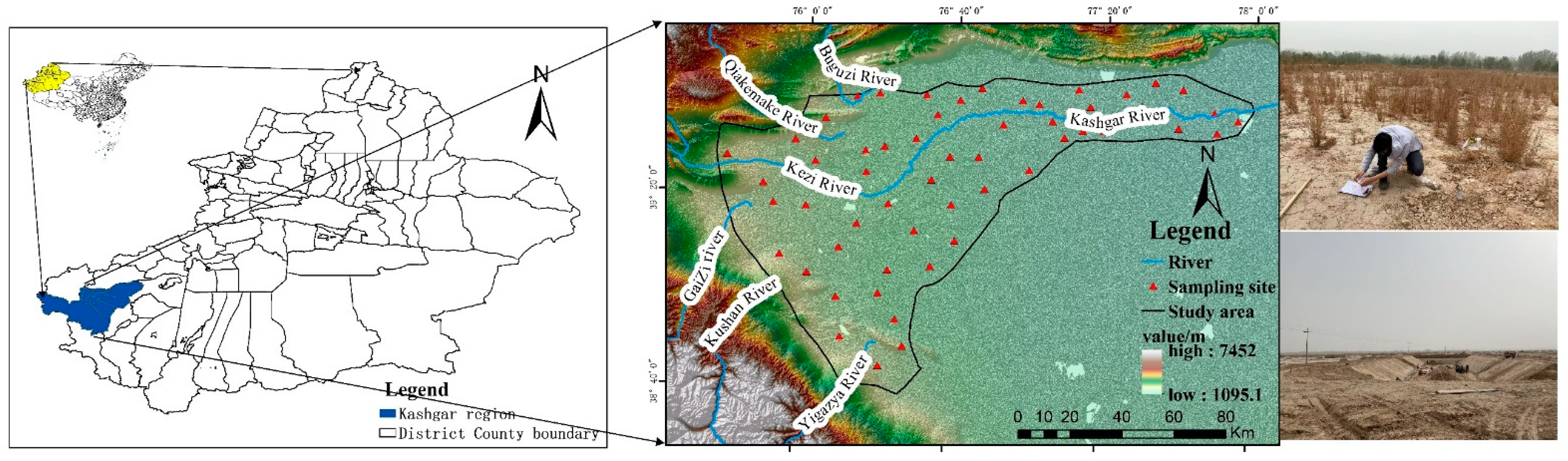
2.1. An Overview of the Study Area

The study area is located in the southwestern part of the Xinjiang Uygur Autonomous Region along the western margin of the Tarim Basin, belonging to the Kashgar River Basin (75°30′0″~78°0′0″ E, 38°40′00″~39°50′00″ N) [22]. The major landforms found in the study area are mountains, dejection cones, alluvial fans, and alluvial–diluvial plain. The study area has four distinct seasons and a long sunshine duration. The majority is located in alluvial–diluvial fan oases, with significant annual and daily temperature changes; the average precipitation over the years is 60.80–172.80 mm with strong evaporation, and the study area belongs to the warm temperate continental arid/semi-arid climate [22]. The main crops grown in the study area are cotton, maize, walnut, and jujube. The natural vegetation includes Tamarix chinensis, Phragmites australis L., Kalidium foliatum, and Haloxylon ammodendron.

2.2. Geological Setting

The Kashgar River basin is located in the composite unit of the east wing of the front arc of Eurasian “mountain” structure and the head of Pamir “evil” structure of Kunlun Mountain in the south, including the geosynclinal fold belt of the southern Tianshan Mountain vein, the Qiaerlong–Kurlang geosynclinal fold belt of the West Kunlun fold system, the Kelpin faulted upfold, and the Tarim depression of the Tarim Platform, with the boundary mostly bounded by regional folds or fault structures.
The quaternary system (Q) is widely distributed in Kashgar River, with the most intense human activities in the basin, and the thickness of the quaternary system changes from 100 to 800 m generally. The particles of quaternary loose sediments gradually become finer from north to south, from west to east, and from south to north, that is, the particles of pebbles > gravel > gravel sand > medium coarse sand > fine sand > silt (sandy loam) > loam (loam) > clay tend to become finer in the plane direction. Vertically, the quaternary loose sediment particles are generally coarse at the top and fine at the bottom.

2.3. Sampling and Testing

Field sampling was conducted in the study area in April 2019, a month when large-scale irrigation activities in the Kashgar River Basin had not yet begun, the evaporation was strong, and the salinization was mostly typical and a representative performance in this study at this time of the year. Fifty-nine sampling sites were set up in this area (Figure 1); to be specific, the sampling point was chosen as the center and another four sampling sites were arranged at a radius of 10 m around the center to form a plum blossom-shaped pattern in order to help reduce variabilities in the soil. Soil samples were sampled in layers of 0–30 cm, 30–50 cm, and 50–80 cm by pedal original earth-drill (with a drill bit 1 cm long and 38 mm in diameter); the soil samples collected from five sampling points were mixed together and about 0.5 kg of the soil sample was preserved while the remaining soil was discarded by quartering. During the sampling process, changes in soil lithology as well as special landforms were recorded in detail. All soil sample bags were numbered and delivered to the laboratory where they were air-dried at room temperature. The soil samples were passed through a 2 mm sieve according to Soil Agricultural Chemical Analysis Methods [23] at a water-to-soil ratio of 5:1. After that, the contents of salt ions (Na+, Cl, HCO3, SO42−, Ca2+, Mg2+, CO3) in the leachate were determined, Cl- was determined by silver nitrate titration, Na+ was determined by flame photometry, HCO3 and CO3 were determined by sulfuric acid titration, SO42− was determined by barium sulfate turbidimetric method, Ca2+ and Mg2+ were determined by atomic absorption spectrophotometry, and the average soil salt concentration was determined by the method of dying residues. The groundwater burial depth and groundwater mineralization data were provided by Xinjiang Survey and Design Institute of Water Resources and Hydropower, with the specific data shown in Table 1.

2.4. Processing Method

2.4.1. Remote Sensing Images

The Landsat 8 satellite images and digital elevation model (DEM) data used for the study were downloaded from a cloud-based data management platform in 10 September 2020 (http://www.gscloud.cn) and had a resolution of 30 m.

2.4.2. Statistical Analysis

Correlation analysis and principal component analysis were performed for soil salinity and constituent ions at the sampling sites using IBM SPSS Statistics 23.0 and Excel 2019.

Principal Component Analysis

Principal component analysis is a multivariate statistical method that reconstitutes the original indexes into a new group of unrelated comprehensive indexes to replace the original indexes by solving the principal components, and uses several comprehensive indexes to reflect the original indexes. Suppose there are n samples and each sample has p indicators, which are recorded as X1, X2, ⋯⋯, XP. The main calculation steps of principal component analysis are as follows:
(1)
Establish the original database.
(2)
Standardize the original data and use the Z-score method to make standard changes to the data:
C i j = x i j x j S j
X = [ x 11 x 1 P x 1 n x n p ]
s j 2 = i = 0 n x ( x i j x j ) 2 n 1   ( j = 1 , 2 ,   , p )
where x i j is the value of the j-th index of the i-th partition and x j , S j are the sample mean and sample standard deviation of the j-th index, respectively.
(3)
Find the correlation coefficient matrix,
R = ( r j k ) p p   ( j ,   k = 1 , 2 ,   , p )
where r j k is the correlation coefficient of indexes j and k.
(4)
Find the eigenvalue and eigenvector of correlation matrix R and determine the principal component. If the characteristic value is recorded as λ 1     λ 2 ≥ ⋯⋯ ≥   λ m ≥ 0, the corresponding unit eigenvector is
a i = ( a 1 i   a 2 i a p i )
Convert the standardized index variables into main components:
Z i = a 1 i   C 1 + a 2 i   C 1 + + a P i   C P   ( i = 1 , 2 ,   , p )
where Z 1 is the first principal component, Z 2 is the second principal component, ⋯⋯; thus, Z p is the p-th principal component.
(5)
Calculate the variance contribution rate and determine the number of principal components. Generally, the number of principal components is equal to the number of original indicators; if the number of original indicators is large, it will be troublesome to conduct comprehensive evaluation. The method of principal component analysis is to select as few k principal components (k < p) as possible for comprehensive evaluation while at the same time making the amount of information lost as little as possible. The contribution rate of the K value from cumulative variance E = i = 1 λ λ i / i = 1 p λ i ≥ 75%, that is, select the minimum k with E ≥ 75%.
(6)
Comprehensive evaluation of K principal components. First find the linear weighted value of each principal component, Z i = a 1 i   C 1 + a 2 i   C 1 + + a P i   C P , (i = 1,2, ⋯⋯, k), Then, the weighted sum of k principal components is obtained to find the final evaluation value: Z = e i Z i , (i = 1,2, ⋯⋯, k) where weight, e i , is the contribution rate of each principal component variance; thus, e i = λ i / i = 1 p λ i .

Correlation Analysis

The measure of the degree of linear correlation between two variables is called the simple correlation coefficient (or single correlation coefficient). For two elements x and y, if their sample values are respectively, x i ,   y i (i = 1,2, ⋯⋯, n), then the correlation coefficient ( r x y ) between them is defined as
r x y = i = 1 n ( x i x ¯ ) ( y i y ¯ ) i = 1 n ( x i x ¯ ) 2 × i = 1 n ( y i y ¯ ) 2

2.4.3. Spatial Data Vectorization

The geographical statistics function was run in ArcGIS to analyze the spatial differentiation structure of groundwater mineralization and burial depth in the study area, and the optimal theoretical model fitted using the variation function was employed for Kriging interpolation to generate the spatial distribution data of groundwater burial depth and mineralization in the study area. ArcGIS 3D Analyst was applied to the DEM data to extract the grid data of the slope in the study area. Landsat-8 optical remote sensing data, which were of the same time period as the field sampling and had undergone atmospheric correction, radiation correction, and geometric correction, were used for land surface temperature inversion. ERDAS software was utilized for the supervised classification of remote sensing images of the same period; in addition, by reference to China’s national standards for land use classification and the actual situation of the study area, we divided the land into the following land use categories: bare land, saline land, shrubbery, low-coverage grassland, and medium-coverage grassland.

2.4.4. Grey Relational Analysis

Grey relational analysis is a multi-factorial statistical analysis method which calculates the similarity between the reference sequence and the comparison sequence; the more similar the two curves, the closer the relation between the sequence will be. This method can be used to quantify the intensity of relation and mutual influence of different factors in a system. The specific methods are as follows [24,25]:
(1)
Original data transformation. The selected indicators are different in physical meanings and dimensions, and we should thus adopt the method of removing dimension before comparing each data column. Each sub-sequence has different effects on the parent sequence; in this paper, we adopted the method of maximum standardization when quantifying standardization of various indicators. For example, there are indicators of positive correlation, such as y i = x i / x 0 , and indicators of negative correlation, such as y i = ( x 0   x i )/ x 0 , where x i is the actual value of the sub-sequence and x 0 is its maximal value.
(2)
Correlation coefficient computations. It is necessary to determine the correlation coefficient ξi(k) in each sub-sequence X i (k) and parent sequence X 0 (k). The computational formula of correlation coefficient in the Grey System is as follows:
ξ i ( k ) = m i n   i m i n k | x 0 ( k ) x i ( k ) | + ρ m a x i m a x k | x 0 ( k ) x i ( k ) | | x 0 ( k ) x i ( k ) | + ρ m a x i m a x k | x 0 ( k ) x i ( k ) |
among which:
k = 0, 1, 2, 3, ⋯, N, i = 0, 1, 2, ⋯7, and ξi(k) is the correlation coefficient of the data series of x i and x 0 at position k. The effect of ρ [0, 1], which is called the resolution ratio, is to highlight the difference between the correlation coefficients. Generally, the resolution ratio is 0.5 [20].
(3)
Solving the correlation degree, r i . The correlation degree of the two sequences is provided by the average value of the correlation coefficient between the sub-sequence and the parent sequence at each time, that is,
  r i = ξ i ( k ) ¯ 1 n k = 1 N ξ i ( k )
where r i is the correlation degree between the two sequences and N is the number of each sub-sequence.

3. Results and Discussion of Research

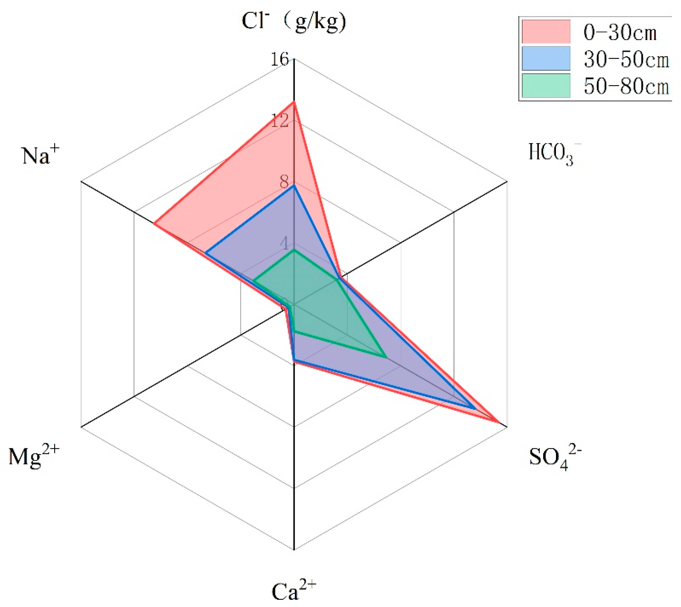
3.1. Analysis of Soil Salt and Ion Content

It can be seen from Table 2 that the average pH of the soil is higher than 8, indicating that the soil is weakly alkaline. The average value of total salt content increases gradually from the deeper layers to topsoil and shows a T-shaped distribution, with the average total salt content of 0 to 30 and 30 to 50 cm soils greater than 20 g/kg and that of 50 to 80 cm soils between 10 and 20 g/kg. According to the local soil salinization classification standard in Xinjiang [26] shown in Table 3, the 0 to 30 and 30 to 50 cm soil horizon are saltierra, and the 50 to 80 cm horizon is severely salinized. Soil salinity is often classified according to the Cl/SO42− concentration ratio [27]; in the study area, the Cl/SO42− concentration ratios of all three horizons were between 0.2–1, and therefore the soil salinity of the wasteland was roughly classified as a chloride–sulfate, which means that the soil salts were predominantly sulfates and chlorides. The radial plot of soil ions (Figure 2) [28] shows that Cl, Na+, and SO42− have vertical differentiation characteristics from top to bottom in the soil profile; in contrast, the contents of other salt ions changed much less significantly in the soil profile. These results indicate that if the climate is dry with little rain and strong evaporation, the salt ions in the wasteland of the river basin tend to accumulate in the surface soil and the soil is rarely washed. In terms of the anions, SO42− has the highest content in all three soil horizons followed by Cl and HCO3; however, the vertical differentiation ability of SO42− is not as good as that of Cl. The content of Na+ in each layer of cation is the largest, followed by the content of Ca2+, and the content of Mg2+ is the lowest (Figure 3).

3.2. Descriptive Statistics and Correlation Analysis of Salt Ions

Because CO32− content is too low, and too low an ion content will cause distortion of coefficient of variation, HCO3 was used in place of soil CO32− + HCO3. The variabilities of salt ion contents across the horizons were compared in order to better understand the differences in the distribution characteristics and migration speeds of different ions in the soil profile [10]; therefore, this paper took the whole section as the research object.
Significant spatial variability in salt ion contents can be observed from Table 4, which might be attributed to the groundwater environment and land use type of the study area. Among the cations, the coefficient of variation was the highest for Na+, among the anions, the coefficient of variation was the highest for Cl, and the contents of both two salt ions showed strong variability. The coefficient of variation was lower for SO42−, Ca2+, and Mg2+, and was the lowest for HCO3; this is similar to the results of previous studies [29]. The reason may be that the vegetation coverage of the wasteland is low and the surface temperature is high; thus, under strong evaporation the soluble salts in soil and groundwater rise with capillary water, and due to the different adsorption capacity of different ions and soil colloids they have different variability and differentiation capacity in the soil profile. Among them, Cl is a conservative ion and Na+ is not easily adsorbed by soil clay; therefore, the coefficient of variation is the largest on the soil profile and is easy to accumulate on the surface. HCO3, SO42−, Ca2+, and Mg2+ are affected by ion charge, hydration radius, ion concentration, and other characteristics, have relatively strong adsorption abilities with soil colloids and relatively small spatial variation [30], and are distributed on the soil profile in a relatively even manner.
A correlation analysis between soil salt ions can help to reveal the existing form and the coordinated migration of salt ions in soil [31]. The correlation coefficients between salt ions are presented in Table 5. It can be seen from Table 5 that the total salt content of the soil is positively correlated with the contents of Cl, SO42− Ca2+, Mg2+, and Na+ with a significance level of 0.01. The pair of anions most strongly correlated is SO42− and Cl, further indicating that sulfates and chlorides are important salts that cause soil salinization; both are negatively correlated with the content of HCO3, with a significance level of 0.01. The hydrolysis of HCO3 is very likely to happen in soil solution, which further aggravates soil alkalinity; from another perspective, we can say that higher salt concentration to some extent helps to inhibit soil alkalinity [32]. Comparing the correlation degrees between salt ions, it was found that Ca2+ is positively correlated with Cl and SO42− with a significance level of 0.01, and the coefficients of correlation were 0.620 and 0.948, respectively. As the cation with the highest content, Na+ has the strongest correlation with Cl (0.989), followed by its correlation with SO42− (0.796), which indicates that the coordinated migration of Na+ and Cl is the strongest, followed by that of Na+ and SO42−. This is consistent with the results of previous studies [10]; in the process of salt moving up and down, chloride and sulfate are the most active substances, mostly in the forms of NaCl and Na2SO4, Carbonate is a minor constituent and is relatively stable in the soil profile. This indirectly indicates that in the process of irrigating and salt-leaching, the leaching rate of chloride is faster than that of other salts; therefore, appropriate irrigation and washing help to reduce the Na+ and Cl contents in the soil and thereby reduce soil salinity [33]. Except for the significant correlation with HCO3, Na+, and Ca2+, where the correlation with HCO3 was the strongest, the correlation between soil pH and other ions was not significant.

3.3. Principal Component Analysis of Salt Ions in the Soil

Due to variabilities of salt ion contents being significant, it was difficult to quantitatively describe the distributions of the various salts and their constituent ions [34]. We performed principal component analysis to identify representative salt factors in the soil and create new variables without causing a loss of the original information, and the principal components thus developed were then used to evaluate the salinized status of the wasteland in the study area to offer a reference for predicting salinity trends during further wasteland reclamation.
After linear transformation, the eigenvalues of the first two principal components were 4.711 and 1.132, both being above 1. The corresponding variance contribution rate was 67.298% and 18.802%, respectively, and the cumulative variance contribution rate was above 85%. These two principal components could cover most of the original data information [31], with the information loss being only 13.9%.
The factor loading matrix in Table 6 shows the degree of correlation between one salt variable and a specific principal component; the higher the loading, the stronger the correlation and the greater the ability of the principal component to cover the information carried by variable [35]. According to the factor loading matrix, SO42−, total salt content, Na+, Cl, Mg2+, and Ca2+ were more strongly correlated with the first principal component, and the factor loadings were 0.922, 0.995, 0.957, 0.928, 0.614, and 0.825, respectively; these salt ions had a very significant positive correlation with the total salt content. From the above, we determined that these six salt variables could represent the salinized status of the soil and the salt ion composition. Therefore, the first principal component could replace the effect of eight variables, excepting only HCO3 and pH. The contribution rate of the first principal component was the largest, oat 67.298%, which shows that the soil is mainly salinized. HCO3 and pH showed high correlation in the second principal component, and the factor load was 0.842 and 0.638; at the same time, HCO3− and pH showed high correlation, indicating that the second principal component had represented the characteristics of salinization of soil and replaced the role of HCO3− and pH in the soil.
The factor loading plot of the first and the second principal components (Figure 3) further reflected that the salinity trend in wasteland of the Kashgar River Basin. Soil salinization was the primary process, while alkalization was secondary.
The coefficients of the principal component score were calculated based on all variables by linear regression analysis; in this way, we could use the linear combinations of principal components and original variables for salinization status evaluation of the wasteland, as shown in Table 6. Hence, we constructed the linear score equations between each principal component and the variables, as shown in Equations (10) and (11).
P1 = 0.211X1 + 0.197X2 + 0.039X3 + 0.196X4 + 0.175X5 + 0.130X6 + 0.203X7 + 0.073X8
P2 = −0.054X1 + 0.046X2 + 0.744X3 − 0.169X4 − 0.325X5 + 0.436X6 + 0.029X7 + 0.073X8
where P1 and P2 are the first and the second principal components, respectively, and X1, X2 to X7, X8 are eight salt variables, namely, total salt content and Cl⋯⋯Na+. By integrating P1 and P2, we further constructed the comprehensive evaluation function of the salinity status of the wasteland of the Kashgar River Basin. As shown in Equation (5), the coefficients in this comprehensive evaluation function were determined by dividing the contribution rate of each of the two principal components by the corresponding cumulative contribution rate.
F1 = 0.781P1 + 0.219P2 = 0.153X1 + 0.164X2 + 0.194X3 + 0.116X4 + 0.066X5 + 0.197X6 + 0165X7 + 0.189X8
The coefficients in the equation above reflected the weights of the principal components and the salt variables in the comprehensive evaluation function; the greater the weights, the more important the variable in the model. The comprehensive score was calculated using Equation (12) for the sampling sites (in the entire soil profile) arranged in the wasteland of the study area; this score varied between 1.556 and 32.140 with an average of 6.20 and a coefficient of variation of 1.12, indicating a strong variation. This result offers a theoretical reference for the comprehensive analysis and evaluation of soil salinity status in the wasteland of the Kashgar River Basin.

3.4. Analysis of the Influence Factors of Salinization

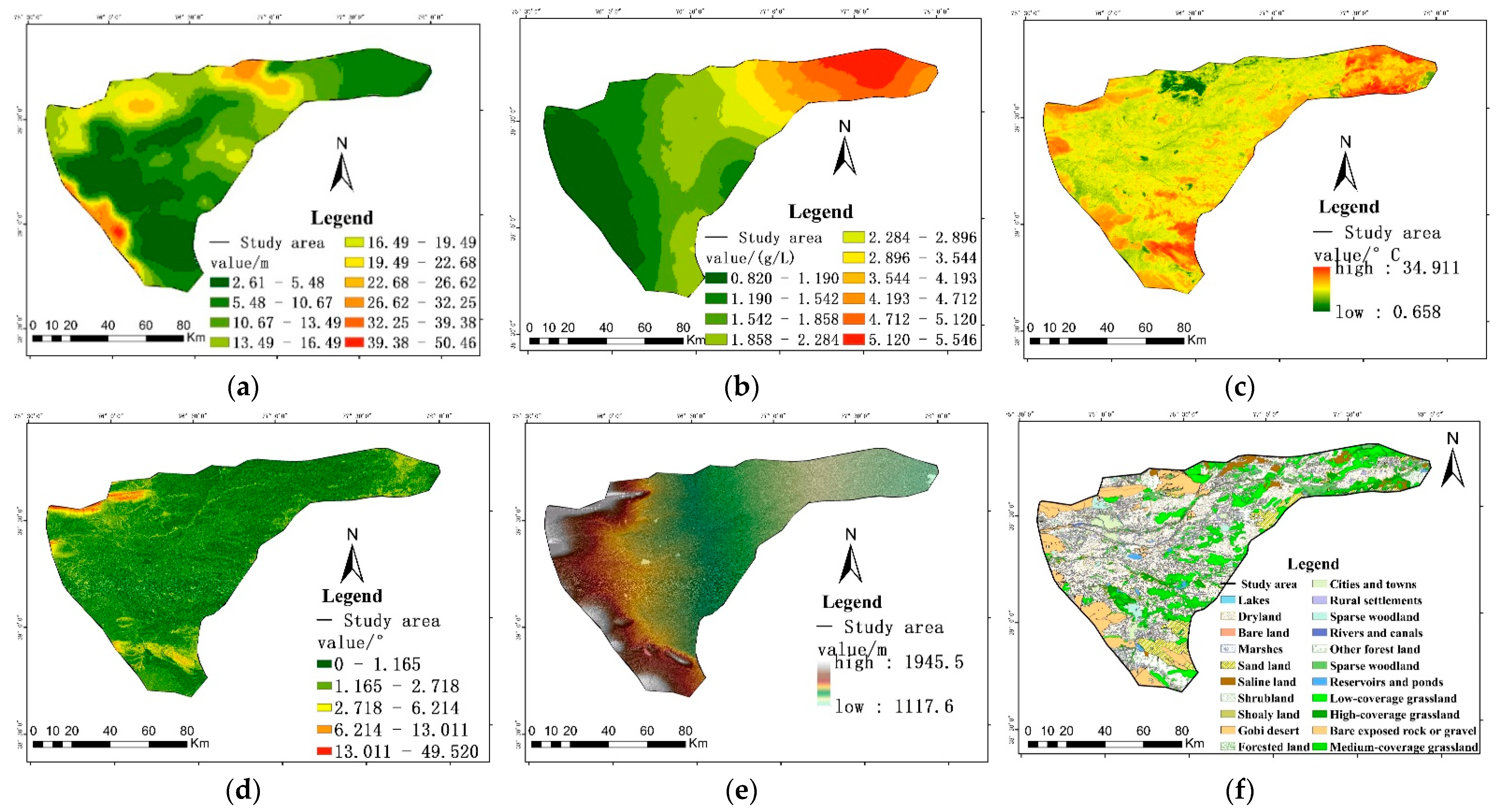
3.4.1. Choice of the Influence Factors of Soil Salinization

The influence factors of soil salinization include meteorological factors, comprehensive geo-science factors, and land management factors. The three types of factors are coupled and jointly act on the soil salinization process [36]. Among them, geo-science (altitude, slope) lays the comprehensive molecular foundation for the formation of salinization, meteorological (surface temperature) and land management factors (mode of land use) influence the trend of salinization, and the groundwater environment has a direct bearing on the salinization process via groundwater mineralization and groundwater burial depth. Therefore, we chose groundwater burial depth, groundwater mineralization, land use type, land surface temperature, elevation, and slope as sequences of influence, and extracted them in terms of their respective spatial variables (Figure 4a–f). The soluble salt content of the sampling point was used as the reference sequence, which was obtained from the indoor analysis results.

3.4.2. Correlation Sequence and Analysis

We calculated the degree of correlation between six types of influencing factors and soil salt content at different depths according to Formulas (8) and (9), as shown in Table 7. In a grey system, the higher the grey relational coefficient, the greater the importance of the factor to salinization formation and evolution; as shown in Table 7, the six influence factors affected soil salinity at different depths in a significantly different manner. In the 0–30 cm horizon, the factors were ranked in descending order of the grey relational coefficient with the soil salt content as follows: land use type > groundwater mineralization > land surface temperature > elevation > groundwater burial depth > slope; in the 30–50 cm horizon, the ranking was as follows: groundwater mineralization > land use type > elevation > land surface temperature > groundwater burial depth > slope; and in the 50–80 cm horizon, the ranking was as follows: groundwater mineralization > elevation > groundwater burial depth > land use type > land surface temperature > slope.
According to Table 7, at a greater soil depth the grey relational coefficient between all influence factors (except for groundwater burial depth and elevation) and the soil salt content gradually decreased; in other words, the 0–30 cm horizon was most susceptible to salinization, and the Grey System coefficients calculated for each influence factor in this horizon represented the sensitivity of each factor and indicated which factors played a greater role in the salinization of shallow soil. In the 0–30 cm horizon, the grey relational coefficients were above 0.7 for the land use type, groundwater mineralization, land surface temperature, and elevation; these four factors were dominant in the evolution of shallow soil salinization. The wasteland, where the soil samples were taken, is mostly composed of saline land, abandoned dryland, grassland, halophyte bush vegetation, and desert. The soil’s physicochemical properties, land surface evaporation intensity (land surface temperature), and physiological characteristics of vegetation vary under different land use types, and it is inevitable that the spatial and temporal distributions of groundwater level and quality are uneven, which further results in differentiation in the intensity of influences on surface soil salinity [37,38,39]. Elevation has a direct impact on groundwater and surface water movement as well as on soil salt accumulation and elimination. As shown in Figure 4, the terrain is higher in the upper reach of the Kashgar River; where the groundwater mineralization is lower, the soil salt discharge is predominant, and the soil salt content is lower. As the groundwater and the surface water move downstream, groundwater mineralization increases and surface soil salinity is further aggravated under strong evaporation. The above findings agree with those by Li [40], Luo [41], and Zhang [42] regarding the influence factors of soil salinity in the Manas River Basin, the oasis of Weigan and Kuqa Rivers, and the Qitai Oasis, respectively.
Compared with surface soils, the relational degree of salt content in the deeper horizon (50–80 cm) with groundwater mineralization and burial depth was greater than that with land use type and land surface temperature. This is probably because the plants and their roots are shorter in the study area. As the roots cannot reach the deeper horizons, the land use type has a greater impact on the salt content of surface soils [17,43]. In areas with shallow buried groundwater, deeper soils are less affected by evaporation (land surface temperature), whereas the capillary action is stronger; thus, in this soil horizon, land use type and land surface temperature had a smaller impact on salinity than groundwater environment. This finding agrees with those of Fan et al. [38,44] In all three horizons, the soil salt content had a lower relational degree with slope, which was different from the results of Zhang et al. [35,42] The reason for this may be attributed to different terrain in different regions; our study area was located in an alluvial-–diluvial plain oasis where the terrain and slope fluctuate less significantly. It can be seen from figure D that the slope is mostly 0–2.718°; therefore, the slope had a lower relational degree with salt content in each soil horizon.

4. Conclusions

Through the statistical analysis, it was found that the wasteland soil in the basin was severely salinized, and the type of saline soil was dominated by surface-aggregate chloride sulfate. There were significant differences in the content and variability of different ions, with Cl and SO42− having the highest content and the greatest variability in anions, indicating that they are rarely affected by irrigation leaching, similar to the results from previous studies. Despite the low carbonate content, the alkalization of the soil is a possibility that should not be neglected. Correlation analysis found that the correlation between the total salt content and Cl, Na+, and SO42− was the strongest. At the same time, the correlation between Na+ and Cl and SO42− were very significant, which reveals that NaCl and Na2SO4 were the main salts in the soil. Due to the easy leaching of chlorides and sodium salts, the contents of Cl, Na+, and SO42− can be reduced by appropriate irrigation and leaching, and the salinization of such soils can be controlled. However, considering that HCO3 is negatively correlated with total salts, rinsing the salt to reduce soil salinity will increase HCO3 content and aggravate soil alkalinity. Therefore, it is necessary to select an appropriate irrigation water quality. The salinization process of the wasteland in the study area is the result of a combination of many factors. Therefore, to scientifically improve and utilize the saline soil in the basin, the focus should be on controlling the influencing factors of salinization in the basin. According to the grey relation analysis, the focus of soil salinity control is to strengthen land use management and prevent inappropriate land development from exacerbating salinization. At the same time, saline soils should be improved by planting salt-tolerant crops and utilizing their desalination effect while ensuring the quality of salt wash water, strengthening dynamic monitoring and regulation of groundwater, maintaining a reasonable groundwater level, and preventing the occurrence of secondary soil salinization caused by improper irrigation and drainage. Finally, the development of soil salinization during the treatment process can be comprehensively assessed through the comprehensive score model (12) constructed by the principal component to provide a scientific basis for subsequent salinization prevention and control.
This study revealed the correlation between total salts of soil and different salt ions, established a linear relationship between different salt ions and principal components, and clarified the influencing factors of salinization. These research results help to reveal the influence of different salt ions on soil salinity, which is the premise and basis for effective prevention and improvement of soil salinity and is of great theoretical and practical significance. In order to better understand the development trend and spatial distribution characteristics of soil salinization in the study area, it will be necessary to further study the spatiotemporal aspects of soil salinity in the next stage of research.

Author Contributions

Conceptualization, S.L. and L.L.; methodology, S.L., Y.G. and D.S.; software, L.L., Y.G. and Y.Z.; validation, Y.G., Y.Z. and L.L.; formal analysis, L.L. and D.S.; investigation, D.S.; resources, S.L.; data curation, Y.Z. and S.L.; writing—original draft preparation, L.L. and Y.G.; writing—review and editing, S.L. and D.S.; visualization, Y.G.; supervision, L.L. and S.L.; project administration, Y.Z.; funding acquisition, S.L. and Y.G. All authors have read and agreed to the published version of the manuscript.

Funding

This research received no external funding.

Institutional Review Board Statement

Not applicable.

Informed Consent Statement

Not applicable.

Data Availability Statement

Some data used during the study are available from the corresponding author by request (email: luli0401@sina.com (L.L.)).

Conflicts of Interest

The authors declare no conflict of interest.

References

  1. Chen, Y.B.; Hu, S.J.; Luo, Y.; Tian, C.Y. Relationship between soil salt accumulation in abandoned surface layer and groundwater in shallow groundwater buried area of Kashgar, Xinjiang. Acta Pedol. Sin. 2014, 51, 75–81. [Google Scholar]
  2. Pérez-Sirvent, C.; Martınez-Sanchez, M.J.; Vidal, J.; Sánchez, A. The role of low-quality irrigation water in the desertification of semi-arid zones in Murcia, SE Spain. Geoderma 2003, 113, 109–125. [Google Scholar] [CrossRef]
  3. Niu, D.L.; Peng, H.C.; Wang, Q.J. The principal component analysis of salinized situation in desert land of Chaidamu basin. Acta Pratac. Sin. 2001, 10, 39–46. [Google Scholar]
  4. Amezketa, E. An integrated methodology for assessing soil salinization, a pre-condition for land desertification. J. Arid Environ. 2006, 67, 594–606. [Google Scholar] [CrossRef]
  5. Dehaan, R.; Taylor, G.R. Image-derived spectral endmembers as indicators of salinization. Int. J. Remote Sens. 2003, 24, 775–794. [Google Scholar] [CrossRef]
  6. Singh, A. Soil salinization management for sustainable development: A review. J. Environ. Manag. 2020, 277, 111383. [Google Scholar] [CrossRef]
  7. Zhao, W.; Zhou, Q.; Tian, Z.; Cui, Y.; Liang, Y.; Wang, H. Apply biochar to ameliorate soda saline-alkali land, improve soil function and increase corn nutrient availability in the Songnen Plain. Sci. Total Environ. 2020, 722, 137428. [Google Scholar] [CrossRef]
  8. Wong, V.N.; Greene, R.S.B.; Dalal, R.C.; Murphy, B.W. Soil carbon dynamics in saline and sodic soils: A review. Soil Use Manag. 2010, 26, 2–11. [Google Scholar] [CrossRef]
  9. Singh, K.; Mishra, A.K.; Singh, B.; Singh, R.P.; Patra, D.D. Tillage Effects on Crop Yield and Physicochemical Properties of Sodic Soils. Land Degr. Dev. 2016, 27, 223–230. [Google Scholar] [CrossRef]
  10. Zhang, T.B.; Kang, Y.H.; Hu, W.; Dou, C.Y. A study on the salinity characteristics of cracked alkaline soil in Yinbei irrigation district of Ningxia based on principal component analysis. Agric. Res. Arid Areas 2012, 30, 39–46. [Google Scholar]
  11. Aly, Z.; Bonn, F.J.; Magagi, R. Analysis of the Backscattering Coefficient of Salt-Affected Soils Using Modeling and RADARSAT-1 SAR Data. IEEE Trans. Geosci. Remote Sens. 2007, 45, 332–341. [Google Scholar] [CrossRef]
  12. Rezaei, A.; Hassani, H.; Fard Mousavi, S.B.; Hassani, S.; Jabbari, N. Assessment of Heavy Metals Contamination in Surface Soils in Meiduk Copper Mine Area, SE Iran. Earth Sci Malays. 2019, 3, 2–8. [Google Scholar] [CrossRef]
  13. Rezaei, A.; Hassani, H.; Fard Mousavi, S.B.; Jabbari, N. Evaluation of Heavy Metals Concentration in Jajarm Bauxite Deposit in Northeast of Iran Using Environmental Pollution Indice. Malays. J. Geosci. 2019, 3, 12–20. [Google Scholar] [CrossRef]
  14. Maiolo, M.; Pantusa, D. Multivariate Analysis of Water Quality Data for Drinking Water Supply Systems. Water 2021, 13, 1766. [Google Scholar] [CrossRef]
  15. Rezapour, S.; Kalashypour, E. Effects of irrigation and cultivation on the chemical indices of saline–sodic soils in a calcareous environment. Int. J. Environ. Sci. Technol. 2019, 16, 1501–1514. [Google Scholar] [CrossRef]
  16. Acosta, J.A.; Faz, A.; Jansen, B.; Kalbitz, K.; Martínez-Martínez, S. Assessment of salinity status in intensively cultivated soils under semiarid climate, Murcia, SE Spain. J. Arid Environ. 2011, 75, 1056–1066. [Google Scholar] [CrossRef]
  17. Li, Y.J.; Ding, J.L.; Gulmira, E. Soil salt distribution and the factors affecting it in the oasis of Weigan and Kuqa Rivers. J. Irrig. Drain. 2019, 3, 58–65. [Google Scholar]
  18. Ding, J.L.; Yao, Y.; Wang, F. Spatial modeling of soil salinization in arid area. Ecol. Environ. 2014, 34, 12. [Google Scholar]
  19. Wu, Z.; Yan, Q.; Zhang, S.; Lei, S.; Lu, Q.; Hua, X. Remote Sensing Monitoring of Soil Salinization Based on SI-Brightness Feature Space and Drivers Analysis: A Case Study of Surface Mining Areas in Semi-Arid Steppe. IEEE Access 2021, 9, 110137–110148. [Google Scholar] [CrossRef]
  20. Liu, S.F. Grey System Theory and Application; Science Press: Beijing, China, 2010. (In Chinese) [Google Scholar]
  21. Elias, J.N.; Shi, Q.D.; Abulah, A.; Xia, N. Quantitative evaluation of Soil Salinization Risk in Yutian Oasis by grey evaluation model. Trans. Chin. Soc. Agric. Eng. 2019, 35, 176–184. [Google Scholar]
  22. Gulgine, H.; Muhtar, T.; Yu, K.; Elsidin, Y.; Aihematijiang, S. Analysis on the characteristics of saline soil of Kashghar river valley. J. Arid Land Resour. Environ. 2012, 26, 169–173. [Google Scholar]
  23. Lu, R.K. Soil Agricultural Chemical Analysis Method; Chinese Agricultural Science and Technology Press: Beijing, China, 1999. (In Chinese) [Google Scholar]
  24. Yao, R.J.; Yang, J.S.; Chen, X.B.; Yu, S.P. Study on risk assessment of soil salinization in typical reclamation area of coastal zone in Northern Jiangsu. Chin. J. Eco-Agric. 2010, 18, 1000–1006. [Google Scholar] [CrossRef]
  25. Maittituerxun, A.; Haimiti, Y.; Sun, H.I. Correlation analysis of the relationship between soil salinity and groundwater in Yili River Basin. Chin. J. Soil Sci. 2013, 44, 561–566. [Google Scholar]
  26. Soil Survey Office of Uygur Autonomous Region of Xinjiang, Agricultural Bureau of Uygur Autonomous Region of Xinjiang. Soil Xinjiang; Science Press: Beijing, China, 1996. (In Chinese)
  27. Li, T.J.; Zhao, Y.; Zhang, K.L. Fundamentals of Soil Science and Soil Geography; People’s Education Press: Beijing, China, 1983. (In Chinese) [Google Scholar]
  28. Iqrahman, A.; Maimaiti, S.; Ma, C.Y. Spatial distribution characteristics of soil salinization in in the oasis of Weigan and Kuqa Rivers. China Rural Water Hydropower 2020, 8, 110–116. [Google Scholar]
  29. Jiao, Y.; Kang, Y.; Wan, S.; Sun, Z.; Liu, W.; Dong, F. Effect of soil matric potential on the distribution of soil salt under drip irrigation on saline and alkaline land in arid regions. Trans. Chin. Soc. Agric. Eng. 2008, 24, 53–58. [Google Scholar]
  30. Xiong, S.G. Basic Soil Science; China Agricultural University Press: Beijing, China, 2001; pp. 185–187. (In Chinese) [Google Scholar]
  31. Liang, D.; Li, X.G.; Asjem, T.; Lai, N. Salinity characteristics of soil profiles in the western lakeside of Bosten Lake, Xinjiang. Agric. Res. Arid Areas 2014, 32, 151–158. [Google Scholar]
  32. Zhang, X.; Huang, B.; Liang, Z.W.; Zhao, Y.C.; Sun, W.X. A study on soil salinization characteristics in the western Songnen Plain. Soils 2013, 45, 1332–1338. [Google Scholar]
  33. Ge, G. Saline Alkali Land Improvement; Water Resources and Electric Power Press: Beijing, China, 1987. (In Chinese) [Google Scholar]
  34. Li, X.G. Analysis of spatial variation characteristics of topsoil salt in the oasis downstream of Kaidu River Basin: Case study of Yanqi County. Geogr. Inform. Sci. 2014, 1, 105–109. [Google Scholar]
  35. Ainur, T. Study on Spatial Variability of Soil Salts in the Bortala River Basin and Its Influence Factors; Xinjiang University: Urumqi, China, 2013. (In Chinese) [Google Scholar]
  36. Liu, Q.; He, Y.; Deng, W.; Zhang, G.X. A study on soil salinization process in a changing environment: A case study of the middle and lower reaches of the Taoer River. J. Arid Land Resour. Environ. 2005, 06, 115–119. [Google Scholar]
  37. Du, B.C.X.; Cheng, Y.X.; Wu, L. Analysis of negative correlation between vegetation and soil salinization in Junggar Basin. Acta Ecol. Sin. 2021, 23, 1–13. [Google Scholar]
  38. Jing, Y.P.; Li, Y.J.; Gao, W.; Li, X.P. Salinity characteristics of saline-alkali soil in Hetao Plain under different land use. Res. Soil Water Conserv. 2020, 27, 372–379. [Google Scholar]
  39. Wang, X.M.; Chai, Z.P.; Tashpolat, T. Spatial heterogeneity of topsoil salinity in the delta oasis of Weigan and Kuqa rivers. J. Arid Land Resour. Environ. 2012, 26, 88–93. [Google Scholar]
  40. Li, Y.Y.; Zhang, F.H.; Pan, X.D.; Chen, F.; Lai, X.Q. Changes of salt accumulation in soil layers with different landforms in Manas River Valley in Xinjiang Region. Trans. Chin. Soc. Agric. Eng. 2007, 23, 60–64. [Google Scholar]
  41. Luo, J.Y. Study on the Impact Factors of Soil Salinization Based on 3S Technology. Master’s Thesis, Xinjiang University, Urumqi, China, 2009; pp. 38–44. (In Chinese). [Google Scholar]
  42. Zhang, F.; Xiong, H.G.; Tian, Y.; Nuan, F.M. Impacts of regional topographic factors on spatial distribution of soil salinization in Qitai Oasis. Res. Environ. Sci. 2011, 24, 731–739. [Google Scholar]
  43. Liu, F.; Chen, P.Y.; Yu, H.C.; Ma, J.Z. Analysis of spatial distribution characteristics of soil water and salts under different land use types in Minqin Oasis. Arid Zone Geogr. 2020, 43, 406–414. [Google Scholar]
  44. Fan, X.M.; Liu, G.H.; Tang, Z.P.; Shu, L.C. Analysis on main contributors influencing soil salinization of Yellow River Delta. J. Soil Water Conserv. 2010, 24, 139–144. [Google Scholar]
Figure 1. Geographical location of the study area and distribution of the sampling sites.
Sustainability 14 03500 g001
Figure 2. Radial diagram of salt ions in the study area [28].
Sustainability 14 03500 g002
Figure 3. Two dimensional factors: load diagram of variable soil salinity.
Sustainability 14 03500 g003
Figure 4. Spatial distribution data of the influence factors of salinization: Groundwater burial depth (a); Groundwater mineralization (TDS) (b); Land surface temperature (LST) (c); Topographic slope (d); Surface elevation (e); Land use type (LUP) (f).
Sustainability 14 03500 g004
Table 1. Groundwater burial depth and groundwater mineralization data for the research area.
NumberXYGroundwater Burial Depth (m)NumberXYTDS (g/L)
P1576,503.94,339,7051.76 T1521,4194,395,7871.49
P2576,067.34,341,2603.20 T2551,4224,333,4440.49
P3572,194.84,340,0688.05 T3569,5244,347,9860.52
P4570,5664,340,27011.46 T4572,8094,373,5541.02
P5571,251.34,341,9274.11 T5604,1834,395,2591.26
P6568,459.74,340,61320.12 T6595,3984,403,9981.17
P7571,176.94,335,6335.34 T7600,9524,337,3181.39
P8570,073.54,330,38130.75 T8607,3064,346,7791.33
P9570,264.34,328,84748.92 T9624,0844,310,9976.45
P10567,675.84,331,74828.50 T10721,2044,400,7905.89
P11565,266.44,331,85054.17 T11648,8744,393,0634.50
P12563,712.44,332,45265.83 T12750,9094,395,2483.20
P13574,753.94,333,6827.05 T13687,9434,327,7181.90
P14551,439.34,326,61213.03 T14688,6034,335,2642.21
P15553,684.74,331,9171.61 T15646,943.14,388,3850.92
P16557,701.64,336,541105.10 T16588,504.84,340,1601.11
P17546,555.34,341,24110.63 T17582,526.94,371,0661.17
P18540,204.24,351,7574.00 T18567,963.64,354,1251.47
P19541,025.14,350,18510.45 T19603,647.14,303,9170.74
P20540,813.94,350,5975.00 T20651,3994,345,7000.69
P21540,548.14,351,1051.40 T21588,620.34,364,7151.46
P22539,247.54,350,8857.70 T22581,8734,377,4391.40
P23538,9384,351,4927.78 T23598,0544,369,1750.75
P24538,620.94,352,1195.60 T24615,9714,376,8563.22
P25551,590.64,346,05622.18 T25583,7114,353,1220.54
P26549,239.84,348,06323.44 T26621,5654,330,5771.95
P27548,058.24,349,22525.38 T27595,8634,356,7782.92
P28546,971.14,345,7153.98 T28605,7854,333,3400.79
P29549,4764,353,53623.44 T29622,4954,354,0052.01
P30550,352.94,352,75820.00 T30603,3384,301,7540.62
P31553,354.64,352,85410.85 T31615,0754,295,8702.42
P32559,470.74,350,7029.50 T32646,5314,370,7104.00
P33568,492.74,344,1057.60 T33654,3274,386,3512.00
P34564,5264,347,7544.16 T34650,9744,362,3720.47
P35565,335.24,349,6744.02 T35622,1214,361,0641.82
P36567,734.64,352,8807.55 T36649,5204,378,1726.55
P37565,471.64,355,39016.00 T37665,6994,371,4353.67
P38570,648.84,347,1312.50 T38636,5424,379,7220.98
P39572,924.54,349,1462.70 T39645,2134,342,5171.32
P40574,453.54,351,0302.70 T40625,9954,349,4955.56
Table 2. Statistical analysis of salt elements in soil profile.
QuantitySoil Depth/cmCl/SO42−pHTotal Salt (g/kg)
590–300.8598.643.64
5530–500.5698.532.29
5750–800.5148.215.82
Table 3. Classification standard of soil salinization degree in Xinjiang [26].
ClassificationNon-SalinizationMild SalinizationModerate SalinizationSevere SalinizationSaltierra
Total salt (g/kg)<33~66~1010~20 >20
Table 4. Descriptive analysis of soil salts and constituent ions.
ItemMinimum
(g/kg)
Maximum
(g/kg)
Mean
(g/kg)
Coefficient of Variation
Cl0.13494.438.0661.995
HCO30.1180.4760.2140.348
SO42−0.24780.1611.8911.121
Ca2+0.08424.5153.0210.834
Mg2+0.0223.4770.4551.08
Na+0.04168.5866.6761.815
Total salt (g/kg)0.078226.3630.351.446
Table 5. Correlation Analysis between soil salinity and composition ions.
ItemClHCO3SO42−Ca2+Mg2+Na+Total Salt (g/kg)
Cl1
HCO30.1431
SO42−0.727 **0.1111
Ca2+0.620 **0.0130.948 **1
Mg2+0.571 **0.266 *0.453 **0.2421
Na+0.989 **0.1600.796 **0.673 **0.568 **1
pH0.3690.413 *0.436−0.402 *−0.2990.400 *1
Total salt (g/kg) 0.945 **−0.362 **0.911 **0.822 **0.552 **0.972 **−0.427
Note: ** p < 0.01, indicating a significant difference; * p < 0.05, indicating a significant difference.
Table 6. Factor loading matrix and factor score coefficient matrix of the principal component analysis.
Salt VariableFactor Loading MatrixFactor Score Coefficient Matrix
Principal Component 1Principal Component 2Principal Component 1Principal Component 2
Total salt content0.995 −0.061 0.211 −0.054
Cl0.928 0.052 0.197 0.046
HCO30.186 0.842 0.039 0.744
SO42−0.922 −0.191 0.196 −0.169
Ca2+0.825 −0.367 0.175 −0.325
Mg2+0.614 0.493 0.130 0.436
Na+0.957 0.033 0.203 0.029
pH0.0820.6280.0730.603
Table 7. Correlations between the influence factors of salinization at different depths.
Depth/cmSubsequence
Groundwater Burial DepthGroundwater MineralizationLand Use TypeLand Surface TemperatureSlopeElevation
0–30 cm0.638 0.762 0.815 0.733 0.597 0.717
30–50 cm0.609 0.723 0.683 0.617 0.503 0.631
50–80 cm0.633 0.698 0.573 0.508 0.498 0.655
Publisher’s Note: MDPI stays neutral with regard to jurisdictional claims in published maps and institutional affiliations.

