Predictive Maintenance Planning for Industry 4.0 Using Machine Learning for Sustainable Manufacturing

Abstract

With the advent of the fourth industrial revolution, the application of artificial intelligence in the manufacturing domain is becoming prevalent. Maintenance is one of the important activities in the manufacturing process, and it requires proper attention. To decrease maintenance costs and to attain sustainable operational management, Predictive Maintenance (PdM) has become important in industries. The principle of PdM is forecasting the next failure; thus, the respective maintenance is scheduled before the predicted failure occurs. In the construction of maintenance management, facility managers generally employ reactive or preventive maintenance mechanisms. However, reactive maintenance does not have the ability to prevent failure and preventive maintenance does not have the ability to predict the future condition of mechanical, electrical, or plumbing components. Therefore, to improve the facilities’ lifespans, such components are repaired in advance. In this paper, a PdM planning model is developed using intelligent methods. The developed method involves five main phases: (a) data cleaning, (b) data normalization, (c) optimal feature selection, (d) prediction network decision-making, and (e) prediction. Initially, the data pertaining to PdM are subjected to data cleaning and normalization in order to arrange the data within a particular limit. Optimal feature selection is performed next, to reduce redundant information. Optimal feature selection is performed using a hybrid of the Jaya algorithm and Sea Lion Optimization (SLnO). As the prediction values differ in range, it is difficult for machine learning or deep learning face to provide accurate results. Thus, a support vector machine (SVM) is used to make decisions regarding the prediction network. The SVM identifies the network in which prediction can be performed for the concerned range. Finally, the prediction is accomplished using a Recurrent Neural Network (RNN). In the RNN, the weight is optimized using the hybrid J-SLnO. A comparative analysis demonstrates that the proposed model can efficiently predict the future condition of components for maintenance planning by using two datasets—aircraft engine and lithium-ion battery datasets.

1. Introduction

With the advent of Industry 4.0, each domain of manufacturing is introducing usage of computers and digitalization, and maintenance is one of them [1,2]. Maintenance is essential because it enhances the lifetime of a device. By introducing maintenance, the lifespan of a system can be extended. Maintenance should be planned in advance with an accurate estimation of the machine failure period to reduce the risk of accidents, financial losses, and human casualties. Predictive Maintenance (PdM) has been commonly used in various sectors, such as manufacturing industries [3], automobile industries [4], and aircraft sectors [5]. Pending equipment failures can be detected and failure time can be predicted in advance with the help of data analytics tools, such as engineering, defined health factors, and statistical inference approaches [6]. Moreover, with PdM, the next failure time can be predicted in a precise manner [7,8].

To examine the construction part of maintenance management in certain timeframes, preventive maintenance is implemented as a calendar-based method that allows facility management (FM) staff to plan properly. However, preventive maintenance is not capable of predicting needed repair parts or a material’s future condition prior to improving the material’s life span, and reactive maintenance does not have the ability to prevent failure [9]. The main objective of PdM is to identify incipient failures and subsequent deterioration by developing the component’s condition using previously acquired information. Therefore, previous activities are considered in determining further maintenance procedures [10]. Note that this type of maintenance is referred to as condition-based maintenance.

In addition, PdM can overcome the abovementioned limitations by anticipating potential faults and replacing components in advance, while the designed materials are still in good condition, in order to prolong their operational life [11]. This strategy relies significantly on functional data gathered by sensors [12,13]. There are two significant methods used to gather information in a facility using continuous surveillance, i.e., monitoring by sensors and monitoring via regular inspections. A combination of different types of data, such as maintenance records, monitoring data, the identification of causes, the knock-on effect of failures, and work orders, is required for PdM decision-making.

In addition to these management techniques, computer-based applications are employed to increase the performance of facility maintenance management (FMM) operations [14]. Machine learning techniques are gaining popularity in manufacturing [15,16]. Currently, computer aided facility management systems (CAFM) [17] and computerized maintenance management systems (CMMS) [18] are well-known construction maintenance models. Both CAFM and CMMS rely on the acquisition of useful data. However, to transfer FM data, Excel spreadsheets and paper-based documents are employed in many cases. However, their use leads to time delays in reacting to service requests, which contribute to inadequate maintenance activities [19].

Building information modelling (BIM) [20] has been used in the architecture, engineering, and construction (AEC)/FM industries to enhance maintenance actions and to store maintenance records, including the problem type and failure locations [21]. Thus, BIM has the ability to increase FMM performance. In addition to BIM, Internet of Things (IoT)-like sensor networks or radio frequency identification (RFID) [22] systems may also collect data on facility situations. The analyst examines PdM issues. For condition-based, corrective, and preventive maintenances, a previous paper [23] introduced a decision support system prototype. However, in the decision support model and the condition prediction models, the process of data incorporation was not considered. Machine learning based techniques are currently becoming prevalent in various applications [24,25]; hence, these techniques can be efficiently applied for PdM.

The primary contributions of this study are as follows:

• The future condition of the components for PdM planning is predicted using optimized deep learning.
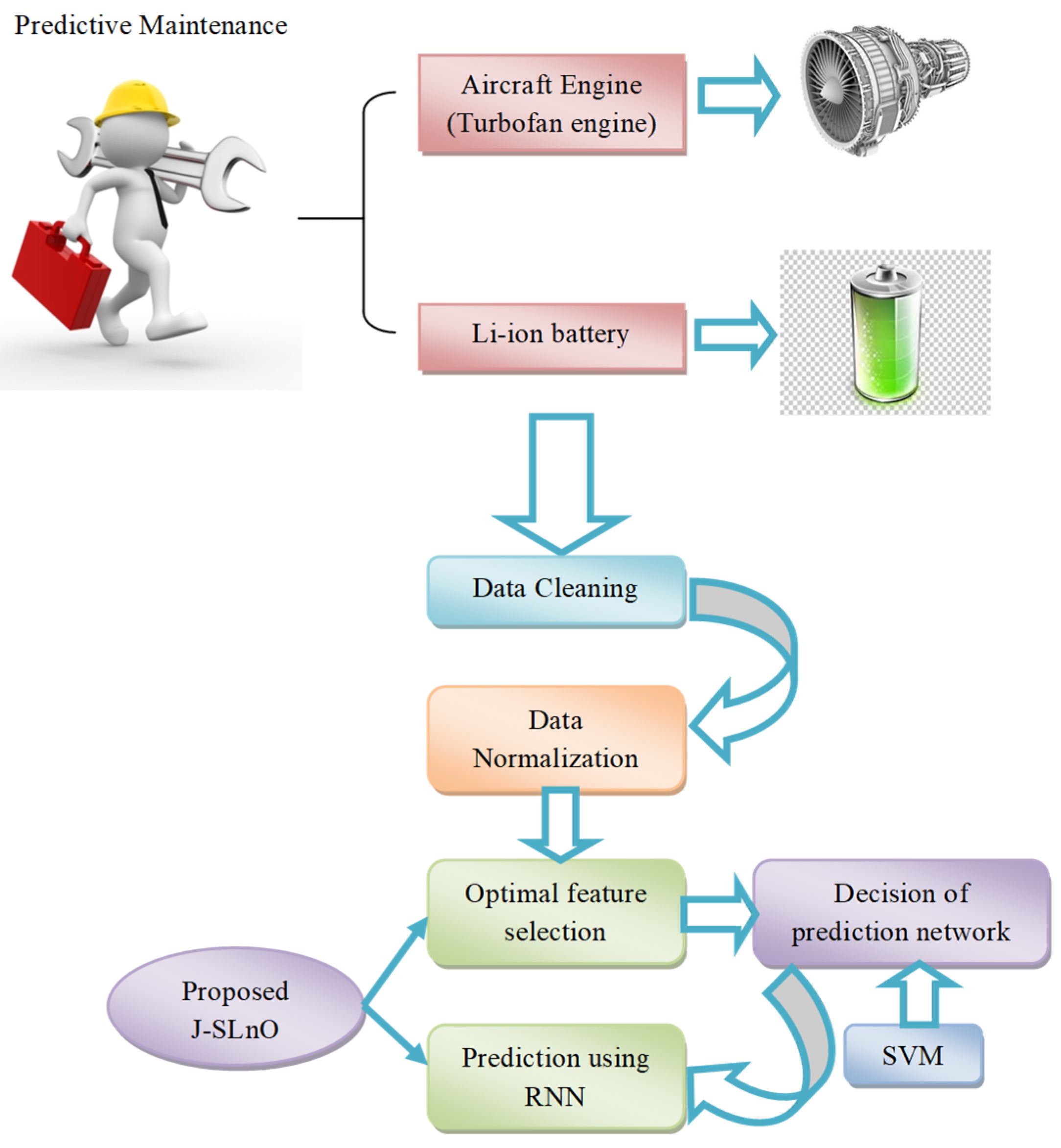
• To improve the prediction in PdM planning, support vector machine (SVM) classification, rather than machine learning algorithms that face complexity when prediction values vary, is used to configure a recurrent neural network (RNN) network for each range of prediction.
• To overcome the problem of overfitting and data redundancy, optimal feature selection is performed using the proposed Jaya-based Sea Lion Optimization (J-SLnO) algorithm. The objective considered for optimal feature selection is to minimize the correlation between two selected features.
• PdM planning performance is improved by modifying an RNN, in which the weight is updated by the proposed J-SLnO algorithm.

The remainder of this paper is organized as follows. Work related to conventional PdM prediction algorithms are discussed in Section 2. PdM planning procedures are described in Section 3. The objective model and optimal feature selection applicable to the proposed PdM planning are discussed in Section 4. Section 5 describes hybrid meta-heuristic algorithms for optimal feature selection and classification. Conclusions and suggestions for future work are provided in Section 7.

2. Literature Review

Chen et al. [26] introduced the Cox proportional hazard deep learning (CoxPHDL) method to resolve data censoring and data sparsity problems related to functional maintenance information analysis. The primary goal of this model was to consider the benefits of reliability optimization and deep learning to deliver an efficient result. Initially, an auto encoder was implemented to transform nominal information into a reliable depiction. Then, to measure the censored information’s time-between-failures (TBF), the Cox proportional hazard model (CoxPHM) was implemented. Based on the preprocessed maintenance information, a long short-term memory (LSTM) network was developed to train the TBF prediction method. Tests were conducted on a “sizable real-world fleet maintenance dataset” to analyze the performance of the proposed model. The results demonstrated that the proposed LSTM network enhanced both the root mean square error (RMSE) and the Matthew’s correlation coefficient (MCC).

Cheng et al. [27] proposed a model based on the BIM and IoT techniques for FMM. This model included application and information layers to obtain the best maintenance performance. In the application layer, there were four modules to accomplish PdM, i.e., a maintenance-planning module, a condition-prediction module, a condition-assessment module, and a condition-monitoring and fault-alarming module; in addition, data integration and collection from the FM system, the IoT network, and the BIM models were performed in the information layer. Both artificial neural networks (ANN) and SVM machine learning algorithms were used to forecast the probable state of the mechanical, electrical, and plumbing modules.

A machine learning approach to perform PdM of a nuclear infrastructure was developed [28]. Here, to predict performance, a logistic regression (LR) and SVM were employed to traverse and compare infrequent events that may be observed in a nuclear structure. The SVM produced the best evaluation measures. In addition, parameter optimization was performed for both the LR and SVM algorithms. This conventional research was conducted on a huge amount of information; however, a new model was introduced to correlate the data of the nuclear infrastructure, in which the probability density was much less.

Susto et al. [6] developed a multiple classifier machine learning methodology for PdM, which is a well-known mechanism for tackling maintenance problems, despite the growing requirement of minimizing downtime and costs. The major problem with PdM was producing the so-called “health factors” of the system’s state that were linked to the provided maintenance problem and that define the association of failure risk with functional costs. This PdM approach enabled the implementation of dynamic decision rules for maintenance management. In addition, it was used to handle censored data and high-dimensional data. The efficiency of this model was demonstrated via simulation and the standard semiconductor manufacturing issue.

Traini et al. [29] discussed the application of a milling cutting-tool PdM solution, which was subjected to real milling datasets to validate the model. Generally, this model provided a basic model to generate a tool to screen wear level, a generic manufacturing tool, and breakdown prevention to enhance production process optimization and human-machine interaction.

A method was proposed based on machine learning models to investigate and visualize offline information from various sources [19]. Here, to recognize clusters, data from three sensors were employed. They demonstrated typical machine tool operations and three defective conditions. In addition, a condition-screening model was developed using these outcomes, which helped to realize the machine tools for PdM solutions.

A random forest (RF)-based machine learning model was proposed by Zenisek et al. [30] to recognize the drifting behavior of presumed concept drifts in continuous data streams. The goal of this model was to recognize wear and tear, as well as subsequent failure, by examining real-time condition-monitoring data reported by sensor-equipped machines. These developments demonstrated the possibility of reducing material and time costs by avoiding failures and enhancing performance. However, there was a need for screening high-quality data to develop computational models. In addition, a new model was introduced to detect the drift concept in data streams as a probable sign of flawed system behavior; the model represented the existing experiments on synthetic datasets.

Markiewicz et al. [31] introduced a new structure in which processing was moved for the sensors themselves to reduce the computational complexity of recurrent neural network (RNN) compression. Here, the data were processed locally by a sensor and then only one packet was transmitted, based on the probability that the machine was operating inaccurately. This structure employed ultra-low power hardware that made it possible for utilizing sensors powered by harvested energy. This structure significantly improved computational power, with low energy consumption.

There are many algorithms to predict necessary maintenance; however, such existing algorithms have several limitations. Thus, a new algorithm must be implemented. The advantages and disadvantages of conventional prediction algorithms are shown in

Table 1. Features and challenges of existing predictive maintenance prediction algorithms.

Author [Citation]	Methodology	Features	Challenges
Chen et al. [26]	LSTM	High performance. Designed to store long-term and short-term pattern data.	Requires more time to train.
Cheng et al. [27]	SVM	Requires less time to solve the problem. More effective than ANNs.	Inappropriate for huge datasets.
Gohel et al. [28]	SVM	Attempts to maximize margin among closest support vectors. High performance.	Does not perform well if the dataset includes noise.
Susto et al. [6]	SVM	Best accuracy. Powerful but complex relative to analysis.	Selecting the kernel function is difficult.
Traini et al. [29]	NN	Best performance. High system reliability.	Hardware dependent.
Uhlmann et al. [19]	Elbow Method	Used to determine cluster count. Reduces distortion and provides precise cluster count.	Performance can be improved.
Zenisek et al. [30]	RF	High performance. Ensembles uncorrelated regression trees provided at random using bagging and boosting to fit the provided information.	Very complex to implement and consumes more time.
Markiewicz et al. [31]	RNN	Reduces computational complexity. Power consumption is reduced.	Computation is quite slow.

. As can be seen, LSTM [26] has high performance and was designed to store long-term and short-term pattern data. However, this technique requires more time for training. SVMs require less time to solve the problem but are more effective than ANNs [6,27,28]. In addition, SVMs attempt to maximize the margins among the closest support vectors, demonstrate high performance and accuracy, and are powerful but complex compared to analysis. However, SVM techniques have several limitations, e.g., they are inappropriate for huge datasets, kernel function selection is difficult, and, if the dataset includes high noise, SVM algorithms do not perform well. Neural networks (NNs) demonstrate high performance and high reliability; however, such methods are hardware dependent [29]. The random forest technique demonstrates high performance, which is realized by employing an ensemble of uncorrelated regression trees provided at random using bagging and boosting to fit the provided information [30]. However, the random forest technique is very complex to implement and requires more time than other techniques. RNNs reduce computational complexity and power consumption [32]; however, the computation is quite slow. Thus, the abovementioned challenges may motivate researchers to develop more effective models for maintenance prediction [31].

3. Procedures for Predictive Maintenance Planning

3.1. Developed Architecture

The PdM approach is implemented for asset maintenance plan optimization by predicting asset failures using data-driven models. Implementing PdM helps to reduce downtime and improve product quality. PdM is also referred to as condition-based maintenance, which attempts to identify failures and eventual degradation via detecting trends in the conditions of components using historical information; thus, fast activities need to be considered. However, PdM has several challenging tasks relative to predicting system failures and repairing components to improve service lifetime. In addition, this method is dependent on collecting and transforming information using sensors. With continuous surveillance and inspection, two methods are used to obtain condition data. In addition, combining different kinds of information, e.g., maintenance records, causes, monitoring data, knock-on effect of failures, and work orders, is required for PdM decision-making. Instead of maintenance methods, computer-based models are employed to enhance FMM activities. The architecture of the proposed PdM planning model is shown in Figure 1.

The proposed PdM planning model employs aircraft engine and lithium-ion battery datasets, which are used to acquire the best prediction details. The proposed model comprises five main phases: (a) data cleaning, (b) data normalization, (c) optimal feature selection, (d) prediction network decision-making, and (e) prediction. First, the datasets are cleaned via outlier detection and filling missing values. Then, the cleaned data are normalized, where the data are arranged within a specific limit (0-1). After normalization, optimal feature selection is performed, where redundant data are removed. Here, optimal feature selection is performed using the proposed J-SLnO algorithm. To provide precise outcomes, machine learning algorithms face complexity because prediction values vary within their ranges. Here, an SVM is employed to obtain a prediction, where the prediction must be performed for the respective range. In addition, the prediction is obtained using an RNN. In RNN-based learning, the weight is optimized by the proposed J-SLnO algorithm.

3.2. Data Cleaning

In data cleaning, errors in the data are detected and repaired by referencing all types of tasks and activities in the data. Here, data cleaning is realized via outlier detection and filling missing values.

Outlier detection [33]. Generally, outliers are considered noisy data in statistics. Several outlier detection models have been introduced for different applications. Some of these methods are more generic than others. Outliers are data patterns that do not represent typical trends in the data. Here, the filloutliers MATLAB function is used to detect outliers and substitute them using a fill method. The outlier detection is carried out for extracting the residual components and decomposing them in early stage.

Missingdata [34]. The missing data problem occurs when some values are missing in the data. Handling missing data requires additional computational time, and the problems caused by missing data require more analysis. To fill missing data, the fillmissing MATLAB function is used to fill missing entries in an array with a constant value. The function performs the decomposition of residuals and approximations. Harmonic analysis is used to decompose the elements into residual and approximate components. Then, data reconstruction is carried out. The main value is taken as the approximation component and a noise component is taken as the residual component. After computing the standard deviation and the mean of the residual component, a random number is computed. Then, the noise components or the sum of the approximation components are utilized for filling in missing data. Finally, this model has reconstructed data.

After outlier detection and filling missing data, the cleaned data are expressed as Dt_u, u = 1, 2, ……, ND, where ND is the total number of target attributes.

3.3. Data Normalization

Data normalization is used to provide normalized information, which replicates several similar records by not changing any values. Data normalization is determined relative to occurrence frequency. Here, record-level normalization produces a representation that is related to records typically observed in the similar record set for a given entity. For each field in the normalized record, field-level normalization selects the value that occurs most frequently.

Once clean data are obtained, the data normalization is performed, which provides various numerical values as output in a given range. Data normalization is described as “adjusting values measured on different scales to a notionally common scale, often prior to averaging.” Here, consider variables be = 0 and ae = 1, where the minimum and maximum normalized values are denoted as be and ae, respectively. The mathematical equation of data normalization is expressed as follows.

$$D{t}_u^{nrm}=\left(ae-be\right)* \frac{\left(D{t}_u-D{t}^{min}\right)}{D{t}^{max}-D{t}^{min}}+be$$

(1)

Here, the normalized data are represented as $D{t}_u^{nrm}$, the value to be normalized is denoted as Dt_u, and the minimum and maximum values for each record are denoted as Dt^min and Dt^max, respectively.

4. Objective Model and Optimal Feature Selection

4.1. Objective Model

There are two objectives that are considered relative to predicting maintenance planning.

Optimal feature selection. The first objective of the proposed PdM model is to select the features that minimize the correlation coefficient in the feature selection process. Here, optimal features are selected from $D{t}_u^{nrm}$, and the objective function of optimal feature selection process is expressed as follows.

$$M1=\begin{array}{c}\mathrm{a}\mathrm{r}\mathrm{g}\\ \left\{D{t}_u^{nrm}\right\}\end{array}\min \left(corr\right)$$

(2)

Here, corr represents correlation. The correlation between features p and q is expressed by Equation (3), where the count of point pairs is given by n.

$$corr=\frac{n{\displaystyle \sum }pq{\displaystyle \sum }p{\displaystyle \sum }q}{\sqrt{(n\sum p^2-{(\sum p)}^2)-(n\sum q^2-{(\sum q)}^2)}}$$

(3)

Optimized RNN: Here, the main objective is to minimize the error between the actual and predicted values. In this case, weight optimization of RNN w_e is performed by the proposed J-SLnO algorithm. The objective function for error minimization is expressed by Equation (4), and the error formula is expressed by Equation (5).

$$M2=\begin{array}{c}\mathrm{a}\mathrm{r}\mathrm{g}\\ \left\{w_e\right\}\end{array}\min \left(err\right)$$

(4)

$$err=D-\widehat{D}$$

(5)

In Equation (5), the actual value is denoted as $\widehat{D}$, and the value predicted by the RNN is denoted as D.

4.2. Optimal Feature Selection

Optimal feature selection is performed after the data have been normalized. Here, as the length of the normalized features appears to be large, optimal feature selection is performed using the proposed J-SLnO algorithm. The solution encoding of the optimal feature selection is shown in Figure 2. The optimal features are denoted as $D{t}_u^{*}$, and the length of the solution is from 1 to the total number of features, denoted as ND.

4.3. SVM-Based RNN Range Classification

In this proposed PdM planning model, the SVM is used to classify the type of RNN based on the prediction range. As per the concept of statistical learning, the SVM [35] is considered the learning model. Here, assume a training set comprising dt data points ${\left\{\left(x_i, y_i\right)\right\}}_{i=1}^{dt}$ with input data $x_i\in {\Re }^n$, and respective binary class labels denoted as $y_i\in \left\{-1,+1\right\}$. As per Vapnik [36], the actual formulation of the SVM classifier satisfies the conditions expressed in Equations (6) and (7).

$$\{\begin{array}{c}{q}^Q\phi \left(x_i\right)+p\ge +1, if y_i=+1\\ q^Q\phi \left(x_i\right)+p\le -1, if y_i=-1\end{array}$$

(6)

$$y_i\lfloor q^Q\phi \left(x_i\right)+p\rfloor \ge 1; i=1,2,\dots \dots ,dt$$

(7)

Here, the non-linear function $\phi (-)$ maps the input space to a huge dimensional feature space. In addition, the above inequalities generally build a hyperplane $q^Q\phi \left(x_i\right)+p$ = 0 that distinguishes two classes. The margin among the two classes is maximized by minimizing $q^{Q}q$. During the primal weight space, the classifier considers the format of Equation (8). As a result, this format is never assessed, and it determines the convex optimization issue. The corresponding equation is expressed in Equation (9), which is subject to Equation (10).

$$y\left(x\right)=sign\lfloor q^Q\phi \left(x\right)+p\rfloor$$

(8)

$$\begin{array}{c}\mathrm{m}\mathrm{i}\mathrm{n}\\ q,p,\xi \end{array}\mathsf{\tau }\left(\mathrm{q},\mathrm{p},\mathsf{\xi }\right)=\frac{1}{2}{q}^{Q}q+Con{\displaystyle \sum }_{i=1}^{dt}{\xi }_i$$

(9)

$$\{\begin{array}{c}{y}_i\left[q^Q\phi \left(x_i\right)+p\right]\ge 1-{\xi }_i i=1,2,\dots .,dt\\ {\xi }_i\ge 0 i=1,2,\dots .,dt\end{array}$$

(10)

Here, the variables ${\xi }_i$ are slack variables that are required to permit misclassifications in the inequality set. In the feature space, the first part of the objective function strives to maximize the margin among the two classes, and the second part minimizes misclassification error. The Con term refers to the positive real constant tuning parameter in the algorithm. Equation (11) expresses the Lagrangian for the restricted optimization issue presented in Equations (9) and (10). This produces the classifier expressed by Equation (12).

$$\begin{array}{c}\mathrm{m}\mathrm{a}\mathrm{x}\\ \alpha ,\nu \end{array}\begin{array}{c} \mathrm{m}\mathrm{i}\mathrm{n}\\ q,p,\xi \end{array} \mathsf{\varsigma }\left(\mathrm{q},\mathrm{p},\mathsf{\xi };\mathsf{\alpha },\mathsf{\nu }\right)$$

(11)

$$y\left(x\right)=sign\left[{\displaystyle \sum }_{i=1}^{dt}{\alpha }_i{y}_{i}C\left(x_i,x\right)+p\right]$$

(12)

Here, the $C\left(x_i,x\right)=\phi {\left(x_i\right)}^Q\phi \left(x\right)$ term is considered by a positive definite kernel that satisfies Mercer’s theorem [37]. By the optimization issue given in Equation (13), the Lagrange multipliers ${\alpha }_i$ are defined and are subject to Equation (14).

$$\begin{array}{c}\mathrm{m}\mathrm{a}\mathrm{x}\\ {\alpha }_i\end{array}-\frac{1}{2}{\displaystyle \sum }_{i,j=1}^{dt}{y}_i{y}_{j}C\left(x_i,x\right){\alpha }_i{\alpha }_j+{\displaystyle \sum }_{i=1}^{dt}{\alpha }_i$$

(13)

$$\{\begin{array}{c}{\displaystyle {\displaystyle \sum }_{i=1}^{dt}}{\alpha }_i{y}_i=0\\ 0\le {\alpha }_i\le Con, i=1,2,\dots ,dt\end{array}$$

(14)

The construction problem of the overall classifier currently facilitates an issue in ${\alpha }_i$ with convex QP. To define the surface’s decision, there is no need to compute q and $\phi \left(x_i\right)$; therefore, the explicit non-linear mapping construction $\phi \left(x\right)$ is required, rather than kernel function C. Generally, kernel function C(.,.) has the choices expressed in Equation (15). Here, the constant terms are denoted as d, c, σ, κ, and θ. Note that the Mercer condition is not satisfied consistently for making note of the multilayer perceptron (MLP) kernel. Several terms of ${\alpha }_i$ are typically equivalent to zero for low-noise issues. In addition, the training observations with respect to non-zero ${\alpha }_i$ are considered support vectors and are positioned very close to the decision boundary.

$$C\left(x,x_i\right)=x_i^{Q}x, \left(Linear Kernel\right)$$

$$C\left(x,x_i\right)={\left(1+\frac{x_i^{Q}x}{c}\right)}^d, \left(Polynomial Kernel\right)$$

$$C\left(x,x_i\right)=exp\left\{-\frac{\left|\right|x-x_i\left|\right|{}_2^2}{{\sigma }^2}\right\}, \left(RBF Kernel\right)$$

$$C\left(x,x_i\right)=\tanh \left(\kappa x_i^{Q}x+\theta \right), \left(MLP Kernel\right)$$

(15)

The SVM classifier is a complex model (Equation (12)), which is considered to have a nonlinear function. It is difficult to grasp classification logics if a nonlinear function is impossible. In such cases, the SVM method must be used; thus, comprehension is significant, and the rules of comprehension are extracted from the trained SVM, which replicates the SVM merely as probable.

5. Hybrid Metaheuristic Algorithms for Optimal Feature Selection and Classification

5.1. Conventional Jaya Algorithm

To demonstrate the working principle of the Jaya algorithm (JA) [38] approach, an infinite benchmark sphere function is considered. Here, the count of design variables is denoted as a at any iteration it, i.e., j = 1, 2, ….., a, and the count of candidate solutions is given as b, which represents the population size c = 1, 2, ….., b. In addition, the best term indicates the best candidate that obtains the best value of f(X) among all candidate solutions, and the worst term refers to the worst candidate, which acquires the worst value of f(X) among all candidate solutions. The value of the b^th variable for the e^th candidate during the it^th iteration is denoted X_{j, c, it} and the value is modified using Equation (16).

$$X_{j,c,it}^{,}=X_{j,c,it}+rnd{1}_{j,it}\left(X_{j,best,it}-\left|X_{j,c,it}\right|\right)-rnd{2}_{j,it}\left(X_{j,worst,it}-\left|X_{j,c,it}\right|\right)$$

(16)

Here, the random numbers are indicated by $rnd{1}_{j,it}$ and $rnd{2}_{j,it}$ for variable j during the it^th iteration, which is in the range [0, 1]. The variable j for the worst and best candidates is denoted as $X_{j,worst,it}$ and $X_{j,best,it}$, respectively. To recognize the values of X_it, this algorithm attempts to minimize the sphere function value. The corresponding equation is expressed in Equation (17), where the X_it is in the range [−100, 100]. The recognized solution for this benchmark function is 0 for the entire values of X_it. The pseudocode for the conventional JA algorithm is given in Algorithm 1.

Algorithm 1.Pseudocode of conventional JA [38].
Initialize the size of population
Find the best and worst solutions
Based on best and worst solutions, modify the solutions using Equation (17).
If $$\left(X_{j,best,it}^{’} is better than X_{j,best,it}\right)$$ (17) While (iteration<maximum number of iterations)
Update the solutions using Equation (17)
	Accept and replace the existing solution
Else
	Maintain the previous solution
End if
If (termination criteria is met)
	Return the optimal solution
Else
	Find best and worst solutions
End

5.2. Conventional Sea Lion Optimization Algorithm (SLnO)

The main motivation of the traditional SLnO [39] algorithm is sea lion hunting behavior. Sea lions are found in huge colonies, where there are several subsets with specific hierarchies. Sea lions can move within these subsets several times in their lives based on their sex, age, and activities. This behavior provides the ability to identify the location of prey and to call other members in the subset to hunt, which is considered as role of the leader for this hunting mechanism while the other lions present in the set update their positions towards the target prey. This method assumes the target prey is the best solution and close to the optimal solution. The mathematical equation of the conventional SLnO optimization algorithm is provided in Equation (18). Here, the dst term indicates the distance between the target and the sea lion, and a random vector that ranges from 0 to 1 is given by rad, which is multiplied by 2 to improve the search space, which allows the search agents to recognize the optimal solution. The tr(it) term refers to the target’s position, and the X(it) term refers to the location of the sea lion. Here, the current iteration is denoted as it.

$$dst=\left|2rad.tr\left(it\right)-X\left(it\right)\right|$$

(18)

In the next iteration, the sea lion moves towards the closest target prey, and this behavior is expressed by Equation (19). The next iteration is given by it + 1, and the constant term is given by C, which is reduced from 2 to 0 in a specific time because this reduces the need for the leader to move toward the current prey and encircle them.

$$X\left(it+1\right)=tr\left(it\right)-dst.C$$

(19)

In the vocalization phase, the sea lions are considered amphibians. In water, the volume of the sound of a lion is four times more than the volume in the air. Sea lions communicate using various sounds when hunting and chasing the subset. In addition, they use specific sounds to identify for other lions that they are on the shore. Here, the sea lions can chase and enclose prey near the surface the ocean. Note that sea lions have very small ears that can hear sounds in and above the water. Thus, prey can be recognized by sea lions, and these lions call other lions to encircle the prey. Equation (20) gives a mathematical representation of the lions’ behavior. Here, the SS_1dr term is the speed of the sound of the sea lion leader’s calls, and the $s{s}_1$ and $s{s}_2$ terms are the speed of sounds in air and water, which are expressed by Equation (21) and Equation (22), respectively.

$$S{S}_{ldr}=\left|\frac{\left(s{s}_1\left(1+s{s}_2\right)\right)}{s{s}_2}\right|$$

(20)

$$s{s}_1=\sin \theta$$

(21)

$$s{s}_2=\sin \varphi$$

(22)

In the attacking phase, sea lions can identify the position of the prey and encircle them. The leader guides the hunting procedure by identifying the prey and informing others about the prey. In most cases, the target prey is the current best-candidate solution. The hunting behavior of sea lions is mathematically represented by a “dwindling encircling mechanism” and “circle updating position.” Based on the value of C, the dwindling encircling process is performed (Equation (23)). The circle-updating location is the chase of sea lions’ bait ball of fish that are hunted starting from the edges (Equation (23)).

$$X\left(it+1\right)=\left|tr\left(it\right)-X\left(it\right)\right|.\cos \left(2\Pi rad\right)+tr\left(it\right)$$

(23)

Here, the distance between the best optimal solution and the search agent is given by $\left|tr\left(it\right)-X\left(it\right)\right|$, || represents the absolute value, and rad is a random number ranging from −1 to 1. To search for prey, sea lions swim with their whiskers zigzagging to randomly recognize the prey. Here, the C term is below one or less than negative one, which forces the sea lions to move away from the target and the sea lion leader. The sea lions update their positions based on the best search agent. However, the search agents update their positions according to randomly selected sea lions. If the C term is greater than 1, the SLnO algorithm applies the global search agent and recognizes the global optimal solution using Equations (24) and (25).

$$dst=\left|2rad.X_{rand}\left(it\right)-X\left(it\right)\right|$$

(24)

$$X\left(it+1\right)=X_{rand}\left(it\right)-dst.A$$

(25)

Here, the random sea lion is denoted as $X_{rand}\left(it\right)$ and selected from the current population. The pseudocode of the conventional SLnO algorithm is given in Algorithm 2.

Algorithm 2.SLnO Algorithm [39].
Start
Population initialization
Choose${\mathit{X}}_{\mathit{r}\mathit{a}\mathit{n}\mathit{d}}$
Compute fitness function for each search agent
The best candidate search agent that has best fitness is the X
while (t < maximum number of iterations)
	Compute $S{\overline{S}}_{ldr}$ using Equation (20)
	if $(S{\overline{S}}_{ldr}<0.25)$
		If $(\left|C\right|<1)$
			Update the location of the current search agent by Equation (18)
		Else
			Choose a random search agent $(X_{rand})$
			Update the location of the current search agent by Equation (25)
	Else
		Update the location of the current search agent by Equation (23)
	Compute the fitness function for each search agent
	Update X if there exists any better solution
	Return X as the best solution
end while

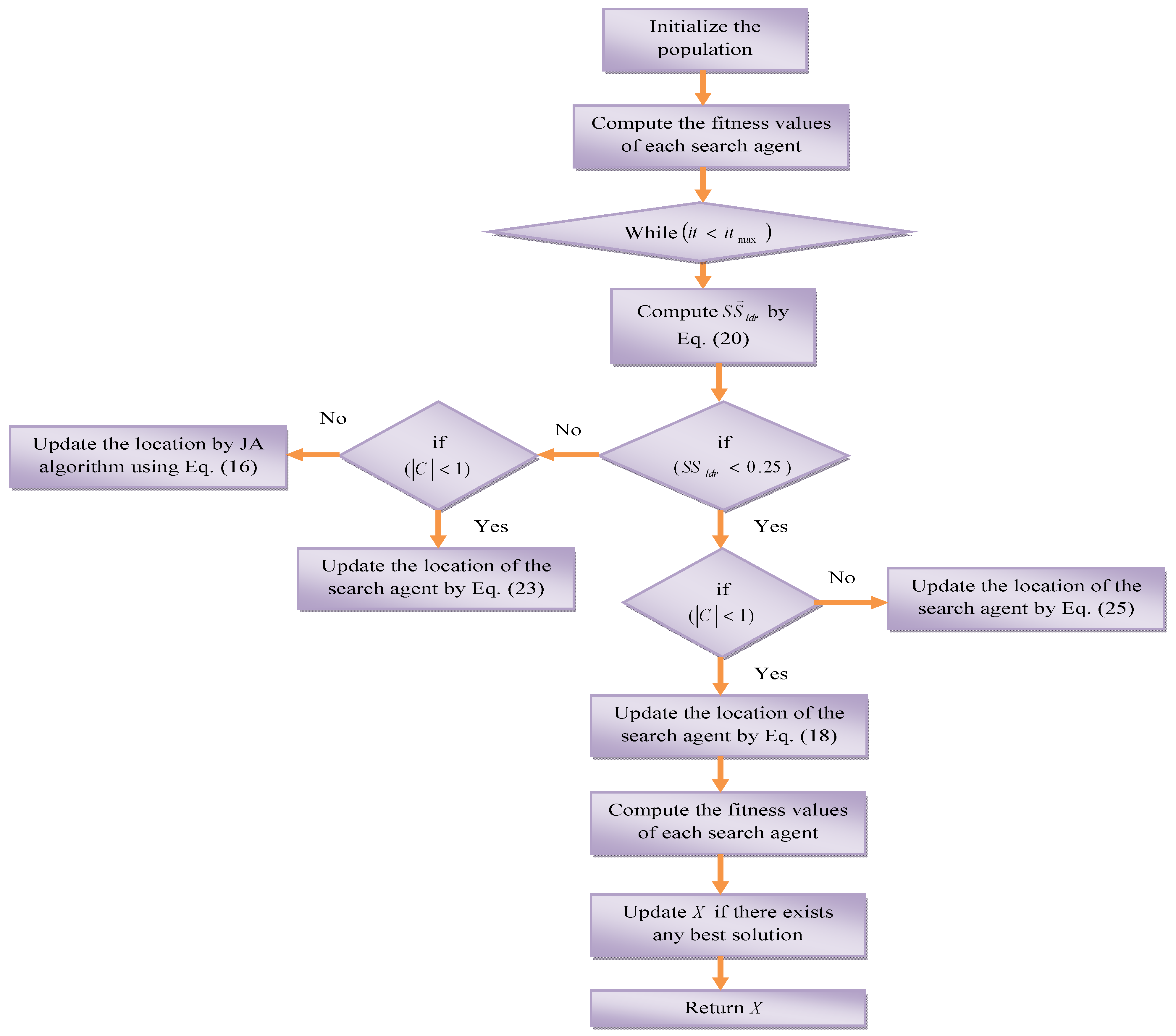
5.3. Proposed J-SLNO Algorithm

The conventional SLnO [39] algorithm was inspired by sea lion hunting behavior, which demonstrates an enhanced hunting strategy, good eyesight, and fast movement. The SLnO algorithm has some advantages, e.g., good exploration capability, and it is efficient in most standard functions. However, the traditional SLnO algorithm also has some disadvantages, e.g., it can easily become trapped in local optima. Thus, to improve the performance of the conventional SLnO algorithm, we have combined it with the Jaya algorithm. This provides the ability to impose regular control parameters, incurs less computation time, and obtains the best accuracy. In the proposed J-SLnO algorithm, if the speed of the sea lion leader’s vocalization is less than 0.25, i.e., $S{\overline{S}}_{ldr}<0.25$, then the typical update process is performed. If $(\left|C\right|<1)$, then the update process of the current search agent is performed using Equation (25). In other cases, the update process is performed using the Jaya algorithm (Equation (16). For some search problems, such hybrid optimization algorithms have produced the best outcomes. The J-SLnO algorithm considers the advantages of various optimization algorithms for fast convergence [40]. The pseudocode of the proposed J-SLnO algorithm is given in Algorithm 3, and a flowchart of the proposed J-SLnO algorithm is shown in Figure 3.

Algorithm 3.J-SLnO Algorithm.
Start
Population initialization
Choose${\mathit{X}}_{\mathit{r}\mathit{a}\mathit{n}\mathit{d}}$
Compute fitness function for each search agent
The best candidate search agent that has the best fitness is the X
while (t < maximum number of iterations)
	Compute $S{\overline{S}}_{ldr}$ using Equation (20)
	if $(S{\overline{S}}_{ldr}<0.25)$
		if $(\left|C\right|<1)$
			Update the location of the current search agent by Equation (18)
		Else
			Choose a random search agent $(X_{rand})$
			Update the location of the current search agent by Equation (25)
	Else
		if $(\left|C\right|<1)$
			Update the location of the current search agent by Equation (23)
		Else
			Update the position by Jaya algorithm using Equation (16)
	Compute the fitness function for each search agent
	Update X if there exists any better solution
	Return X as the best solution
end while

5.4. Recurrent Neural Network

Here, a deep learning model, i.e., an RNN [41], is adopted to perform prediction in PdM planning. In general, an RNN is a type of ANN, where the association among the nodes generates a directed graph with the progression information. RNNs can use time series data effectively; therefore, the best results are found during the earlier and the current data regulation. An RNN uses LSTM architecture and each LSTM unit contains a memory cell that includes an output, forget, and input gates. RNNs are employed to solve the gradient explosion problem and handle massive amounts of data. LSTM removes unnecessary data and the required data are captured when the memory cell state is updated. Here, a gated recurrent unit (GRU) is used in the LSTM. The GRU is used to build the RNN for performance improvement. These combine the output and forget gates into a unique update gate, $u{p}_g$, where the linear interpolation helps acquire the current outcome. Let $e_g\leftarrow D{t}_u^{*}$ be the input feature of g and the earlier hidden state, given by $hd{n}_{g-1}$. Expressions for the update and the reset gates are given in Equations (26) and (27), respectively. Here, the activation function is given by af, which is a logistic sigmoid function. The weight matrix is denoted as $w_e=\left\{w^{eupg}, w^{fup},w^{erg},w^{frg}\right\}$, and it is optimized for error variance minimization among the actual and forecast results using the proposed J-SLnO algorithm.

$$u{p}_g=af\left(w^{eup}{e}_g+w^{fup}{f}_{f-1}\right)$$

(26)

$$r{g}_g=af\left(w^{erg}{e}_g+w^{frg}{f}_{f-1}\right)$$

(27)

In Equation (28), the candidate state of the hidden unit is measured. Here, $\otimes$ refers to the element-wise product. The linear interpolation and the candidate state are denoted by f_g−1 and f_g, respectively. The g^th hidden activation function is the hidden state of f_g of the GRU (Equation (29)).

$${\tilde{f}}_g=tan\left(w^{ef}{e}_g+w^{ff}\left(f_{g-1}\otimes r{g}_g\right)\right)$$

(28)

$$f_g=\left(1-u{p}_g\right)\otimes {\tilde{f}}_g+u{p}_g\otimes f_{g-1}{f}_g=\left(1-u{p}_g\right)\otimes {\tilde{f}}_g+u{p}_g\otimes f_{g-1}$$

(29)

A diagrammatic representation of the process by which the weight is determined is shown in Figure 4.

Thus, the weight of the RNN is optimized using the developed J-SLnO algorithm to improve performance.

6. Results and Discussion

6.1. Experimental Setup

The developed PdM planning process using an SVM and optimized RNN was implemented using MATLAB 2018a. Aircraft engine and Li-ion battery datasets were used to evaluate the performance of the proposed model.

Dataset 1: The aircraft engine dataset was gathered from Github [42]. It included several multi-variate time series data, which ranged from different engines including 100 engines. The lengths of the run varied, with a minimum of 128 cycles and a maximum length of 356 cycles.

Dataset 2: Li-ion cells (18,650) with a nominal capacity of 2 Ah were cycled in a range of ambient temperatures (4 °C, 24 °C, and 43 °C), charged with a common CC-CV protocol and with different discharging regimes. The dataset included in-cycle measurements of terminal current, voltage and cell temperature, and cycle-to-cycle measurements of discharge capacity and EIS impedance readings.

The proposed J-SLnO algorithm was compared to conventional meta-heuristic-based RNNs, i.e., particle swarm optimization (PSO)-RNNs [43], grey wolf optimization (GWO)-RNNs [44], JA-RNNs [38], and SLnO-RNNs [39]. The performance analysis was compared to other machine learning algorithms, such as NN [45,46], KNN [47], RNN [41], and SVM-RNN [35]. Here, the performance analysis considered various performance measures, i.e., mean error percentage (MEP), symmetric mean absolute percentage error (SMAPE), mean absolute scaled error (MASE), mean absolute error (MAE), root mean square error (RMSE), L1 Norm, L2 Norm, and L-Infinity Norm.

6.2. Error Measures

Eight error metrics are considered in the evaluation, and are explained as follows:

(i) MEP: MEP is the calculated average of the percentage of errors between a model’s forecasts and the actual value of the quantity being forecast. In the MEP calculation, Fv is the forecast value, Av is the actual value, j is the number of fitted points, and i is the value added for each fitted point.

$$MEP=\frac{100\%}{j}{\displaystyle \sum }_{i=1}^j\frac{Av-Fv}{av}$$

(30)

(ii) MAE: The MAE is a metric for comparing two continuous variables.

$$MAE=\frac{{{\displaystyle \sum }}_{i=1}^j\left|F{v}_i-A{v}_i\right|}{j}$$

(31)

(iii) SMAPE: SMAPE is a percentage error-based accuracy metric.

$$SMAPE=\frac{100\%}{j}{\displaystyle \sum }_{i=1}^j\frac{\left|Fv-Av\right|}{\frac{\left(\left|Av\right|+\left|Fv\right|\right)}{2}}$$

(32)

(iv) MASE: The MAE of the prediction values is divided by the MAE of the one-step naive forecast in the sample to estimate the MASE.

$$MASE=mean\left(\frac{\left|Fv\right|}{\frac{1}{j-1} {{\displaystyle \sum }}_{i=1}^j\left|A{v}_i-A{v}_{i-1}\right|}\right)$$

(33)

(v) RMSE: RMSE is a commonly used metric for comparing values predicted by a model or to estimate observed values.

$$RMSE=\sqrt{\frac{{{\displaystyle \sum }}_{i=1}^j{\left(A{v}_{i2}-F{v}_{i1}\right)}^2}{j}}$$

(34)

(vi) L1 Norm: The sum of the magnitudes of the vectors in a space is the L1 Norm. Here, the term L is a matrix, t = 1,2,…., n, where n is the size of the matrix.

$$L1={\displaystyle \sum }_i\left|L_i\right|$$

(35)

(vii) L2 Norm: The L2 Norm is the shortest distance between two points. It is also known as the Euclidean norm.

$$L2={\left({\displaystyle \sum }_{i=1}^j{L}_i^2\right)}^{\frac{1}{2}}$$

(36)

(viii) L-Infinity Norm: The maximal norm can be used to compute the length of a vector. The L-Infinity norm is also called the Max norm.

$$L_{inf}=\underset{1\le i\le j}{\max }\left|L_i\right|$$

(37)

6.3. Meta-Heuristics-Based RNN for PdM Planning

The analysis of the proposed and the conventional meta-heuristic-based RNN with respect to the learning percentage for the two datasets is shown in Figure 5 and Figure 6. As shown in Figure 5a, based on the MEP, the developed J-SLnO-RNN algorithm accurately predicts the values. The MEP of the proposed J-SLnO-RNN algorithm was 34.6% better than the PSO-RNN, 51% better than the SLnO-RNN, 62.3% better than the JA-RNN, and 67.3% better than the GWO-RNN at learning percentage 35. When considering any learning percentage, the proposed J-SLnO-RNN algorithm achieved the best performance, as shown in Figure 5c. At learning percentage 65, the MASE of the introduced J-SLnO-RNN was 72.2% superior to that of the SLnO-RNN, 83.3% superior to that of the GWO-RNN, 87.8% better than that of the JA-RNN, and 92.8% better than that of the PSO-RNN. As shown in Figure 5e, the proposed J-SLnO-RNN performed well compared to other algorithms, when considering any of the learning percentages. Thus, the RMSE of the improved J-SLnO-RNN was 15.2% better than that of the SLnO-RNN, 18% better than that of the PSO-RNN, and 28.5% better than that of the GWO-RNN at learning percentage 85. Moreover, at a learning percentage of 85%, the L1-Norm of the proposed J-SLnO-RNN was 8.3% better than that of the SLnO-RNN, 15.3% better than that of the PSO-RNN, and 26.6% better than that of the GWO-RNN. In addition, the performance analysis of the developed J-SLnO-RNN with respect to learning percentage is shown in Figure 6. As can be seen in Figure 6c, the MASE of the improved J-SLnO-RNN was 80%, 83.3%, and 88.8% better than those of the GWO-RNN, the JA-RNN, and the SLnO-RNN, respectively, when considering the learning percentage as 35. At learning percentage 85, the RMSE of the hybrid J-SLnO-RNN was 85.7% better than that of the PSO, 86.6% better than that of the SLnO, 90.7% better than that of the GWO, and 92% better than that of the JA-RNN, as shown in Figure 6e. The L1 Norm of the proposed J-SLnO-RNN algorithm was 46.6% better than that of the GWO-RNN, 60% better than that of the JA-RNN, and 73.3% better than that of the SLnO-RNN at learning percentage 35, as shown in Figure 6f. Moreover, based on an evaluation using the two datasets, the overall performance of the proposed and conventional meta-heuristic algorithms is shown in

Table 2. Overall performance analysis of various meta-heuristic-based RNNs for predictive maintenance planning using the aircraft engine dataset.

Error Measures	PSO-RNN [43]	GWO-RNN [44]	JA-RNN [38]	SLnO-RNN [39]	J-SLnO-RNN
MEP	123.47	96.037	215.55	105.05	82.84
SMAPE	1.0408	0.75052	0.65396	0.65884	0.51309
MASE	1.3655	5.9667	4.9249	6.0355	1.7978
MAE	50.058	40.795	43.281	36.004	28.296
RMSE	64.307	53.641	53.204	46.857	41.742
L1 Norm	1.64 × 105	1.34 × 105	1.42 × 105	1.18 × 105	92,643
L2 Norm	3679.6	3069.2	3044.3	2681.1	2388.4
L-Infinity Norm	184.72	131.9	115.64	118.7	121.45

and

Table 3. Overall performance analysis of various meta-heuristic-based RNNs for predictive maintenance planning using the Li-ion battery dataset.

Error Measures	PSO-RNN [43]	GWO-RNN [44]	JA-RNN [38]	SLnO-RNN [39]	J-SLnO-RNN
MEP	5.4193	6.3721	3.1873	10.32	2.7151
SMAPE	0.040926	0.049924	0.030704	0.090627	0.025625
MASE	0.7249	0.68541	0.32876	0.80602	0.28758
MAE	30.152	37.854	26.658	74.992	18.781
RMSE	83.115	89.443	48.334	114.59	35.396
L1 Norm	9.35 × 102	1.17 × 103	8.26 × 102	2.32 × 103	582.22
L2 Norm	462.76	498	269.11	638	197.08
L-Infinity Norm	434.65	455.95	214.22	443.43	136.02

. In Table 2, the SMAPE of the suggested J-SLnO-RNN obtained the best prediction accuracy when compared to the other algorithms. J-SLnO-RNN was 50.7% better than PSO-RNN, 31.6% better than GWO-RNN, 21.5% better than JA-RNN, and 22.1% better than SLnO-RNN. Similarly, the RMSE of the hybrid J-SLnO-RNN algorithm was 35% better than that of the PSO, 22.1% better than that of the GWO, 21.5% better than that of the JA, and 10.1% better than that of the SLnO-based RNN. In addition, the MASE of the proposed J-SLnO-RNN for the Li-ion battery dataset (Table 3) was 60.3% better than that of the PSO, 58% better than that of the GWO, 12.5% better than that of the JA, and 64.3% better than that of the SLnO-RNN. In Table 3, the RMSE of the proposed J-SLnO-RNN was 57.4%, 60.4%, 26.7%, and 69.1% better than those of the PSO-RNN, the GWO-RNN, the JA-RNN, and the SLnO-RNN, respectively. Thus, it is concluded that the proposed J-SLnO-RNN is superior to conventional RNNs in predicting the maintenance planning.

6.4. Machine Learning Algorithms for PdM Planning

The analysis of the proposed and the traditional machine learning algorithms with respect to learning percentage for the two datasets for PdM planning is graphically represented in Figure 7 and Figure 8, respectively. From Figure 7a, it is evident that the MEP of the proposed J-SLnO-RNN is an efficient method for forecasting maintenance. It was 27.2% better than the SVM-RNN, 40.7% better than the RNN, 46.6% better than the k-nearest neighbors (KNN), and 38.4% better than the NN when considering the learning percentage is 85. At learning percentage 35, the MAE of the proposed J-SLnO-RNN was 20% better than that of the SVM-RNN, 39.1% better than that of the RNN, 33.3% better than that of the KNN, and 12.5% better than that of the NN, as shown in Figure 7d. Moreover, the RMSE of the proposed J-SLnO-RNN achieved the best performance at any learning percentage. Considering a learning percentage of 75%, the RMSE of the improved J-SLnO-RNN was 18% better than that of the SVM-RNN, 45.3% better than that of the RNN, 25.4% better than that of the KNN, and 2.5% better than that of the NN, as shown in Figure 7e. Similarly, the analysis of the proposed and machine learning algorithms for the Li-ion battery dataset is shown in Figure 8. From Figure 8b, it is evident that the SMAPE of the developed J-SLnO-RNN at learning percentage 35 was 25% improved compared with that of the SVM-RNN, 92.5% improved compared with that of the RNN, 78.5% improved compared with that of the KNN, and 82.3% improved compared with that of the NN. At learning percentage 85, the MASE of the suggested J-SLnO-RNN in Figure 8c was 83.3% superior to that of the SVM-RNN, 50% superior to that of the RNN, 36.3% superior to that of the KNN, and 45.4% superior to that of the NN. In Figure 8e, the RMSE of the introduced J-SLnO-RNN is 50% more progressed than that of the SVM-RNN, 96.2% more progressed than that of the RNN, and 93.3% more progressed than that of the KNN and the NN, when considering the learning percentage as 35. The overall classification analysis of the implemented J-SLnO-RNN and the conventional machine learning algorithms for the two datasets is shown in

Table 4. Overall analysis of different machine learning algorithms for predictive maintenance planning using the aircraft engine dataset.

Error Measures	NN [45]	KNN [47]	RNN [41]	SVM-RNN [35,41]	J-SLnO-RNN
MEP	128.31	143.48	173.64	106.95	82.84
SMAPE	0.58454	0.72322	0.96011	0.64453	0.51309
MASE	2.3749	0.91535	0.96928	3.8597	1.7978
MAE	33.419	42.884	56.886	35.794	28.296
RMSE	38.837	54.74	74.34	49.105	41.742
L1 Norm	1.09 × 105	1.40 × 105	1.86 × 105	1.17 × 105	92,643
L2 Norm	2222.2	3132.2	4252.3	2809.7	2388.4
L-Infinity Norm	99.519	137	284.49	133.34	121.45

and

Table 5. Overall analysis of different machine learning algorithms for predictive maintenance planning using the Li-ion battery dataset.

Error Measures	NN [45]	KNN [47]	RNN [41]	SVM-RNN [35,41]	J-SLnO-RNN
MEP	25.723	16.429	54.028	5.4725	2.7151
SMAPE	0.20028	0.12222	0.36893	0.037398	0.025625
MASE	0.57038	0.23407	0.96412	1.153	0.28758
MAE	546.08	316.3	931.43	27.119	18.781
RMSE	762.47	724.61	1164.4	92.844	35.396
L1 Norm	87,373	50,608	1.47 × 105	840.7	582.22
L2 Norm	9.64 × 103	9.17 × 103	1.46 × 104	5.17 × 102	197.08
L-Infinity Norm	2044.2	2284	3759.9	509.26	136.02

. As can be seen in Table 4, the MEP of the presented J-SLnO-RNN was 15.3% better than that of the NN, 34% better than that of the KNN, 50.2% better than that of the RNN, and 20.9% better than that of the SVM-RNN. Moreover, the RMSE of the introduced J-SLnO-RNN was 7.4% more enhanced than that of the NN, 23.7% more enhanced than that of the KNN, 43.8% more enhanced than that of the RNN, and 14.9% more enhanced than that of the SVM-RNN. For the Li-ion battery dataset, the overall performance analysis of the proposed and the traditional classifiers is shown in Table 5. Here, the SMAPE of the suggested J-SLnO-RNN was 87.2% improved compared with that of the NN, 779% improved compared with that of the KNN, 93% improved compared with that of the RNN, and 31.4% improved compared with that of the SVM-RNN. In addition, the RMSE of the implemented J-SLnO-RNN algorithm was 95.3% more advanced than that of the NN, 95.1% more advanced than that of the KNN, 96.9% more advanced than that of the RNN, and 61.8% more advanced than that of the SVM-RNN. Therefore, the above analysis proved that the developed J-SLnO-RNN achieved the best prediction performance for maintenance planning.

6.5. Analysis on K-Fold Validation for PdM Planning

The analysis on the proposed and the conventional meta-heuristic-based RNN and machine learning algorithms in terms of K-fold validation with respect to the learning percentage for the two datasets is shown in

Table 6. K-fold analysis of different optimization algorithms for predictive maintenance planning on both datasets.

Error Measures	PSO-RNN [43]	GWO-RNN [44]	JA-RNN [38]	SLnO-RNN [39]	J-SLnO-RNN
Aircraft Dataset
MEP	1.8765	1.8345	1.7773	1.7868	1.6914
SMAPE	0.021446	0.020966	0.020312	0.020421	0.01933
MASE	0.026873	0.025767	0.025107	0.025299	0.024076
MAE	1.2525	1.2044	1.1728	1.1848	1.1259
RMSE	5.3746	5.249	5.1909	5.1776	5.0895
L1 Norm	16,403	15,773	15,359	15,517	14,745
L2 Norm	615.06	600.68	594.04	592.51	582.44
L-Infinity Norm	22.58	24.69	32.71	19.45	15.62
Li-ion battery Dataset
MEP	1.9501	1.8721	1.8331	1.7551	1.6381
SMAPE	0.022287	0.021395	0.020949	0.020058	0.018721
MASE	0.049074	0.049092	0.045265	0.044557	0.04046
MAE	56.975	57.66	53.047	51.514	47.221
RMSE	218.81	222.43	212.05	211.73	196.02
L1 Norm	36,521	36,960	34,003	33,021	30,269
L2 Norm	5539.9	5631.6	5368.8	5360.6	4962.8
L-Infinity Norm	966	967.25	966.25	967.25	965.25

and

Table 7. K-fold analysis of different machine learning algorithms for predictive maintenance planning for both datasets.

Error Measures	NN [45]	KNN [47]	RNN [41]	SVM-RNN [35,41]	J-SLnO-RNN
Aircraft Dataset
MEP	1.9739	2.0865	1.9911	2.0197	1.6914
SMAPE	0.022559	0.023846	0.022755	0.023082	0.01933
MASE	0.027648	0.030027	0.029407	0.028053	0.024076
MAE	1.2914	1.4027	1.3717	1.3104	1.1259
RMSE	5.3765	5.6753	5.6403	5.4632	5.0895
L1 Norm	16,913	18,369	17,964	17,161	14,745
L2 Norm	615.27	649.46	645.46	625.2	582.44
L-Infinity Norm	26.28	27.31	36.25	22.54	18.21
Li-ion battery Dataset
MEP	1.9111	2.0281	1.9501	2.0281	1.6381
SMAPE	0.021841	0.023178	0.022287	0.023178	0.018721
MASE	0.048692	0.052466	0.047627	0.049824	0.04046
MAE	57.209	60.038	55.99	58.299	47.221
RMSE	219.16	224.91	214.64	222.39	196.02
L1 Norm	36671	38484	35890	37370	30269
L2 Norm	5548.6	5694.2	5434.2	5630.5	4962.8
L-Infinity Norm	975	970.5	973.75	973.75	965.25

, respectively. From this analysis, the efficient performance is observed for the designed model, compared toother existing algorithms in terms of several performance metrics.

7. Discussion

This paper has proposed a J-SLnO algorithm for improving the performance an intelligent PdM planning model with the abilities of the SLnO algorithm. Although the existing algorithm pose a vast range of benefits in various fields, they suffer from various challenges in existing studies. Therefore, the existing algorithms achieve lower performance in the proposed model, when compared to the new improved algorithm. The PSO algorithm has a simple theory, easier implementation, computational efficiency, and robustness to control parameters. However, it suffers from a lower convergence rate and easily falls into local optima. The GWO was selected for comparison due to its simplicity, employing fewer control parameters, and ease of implementation; the GWO has been widely applied to solve different optimization problems, such as parameters estimation. It faces complications in alleviating the lack of population diversity, the imbalance between exploitation and exploration, and premature convergence of the GWO algorithm. The NN has the ability of training the machine, the capability of parallel processing, superior fault tolerance, and stores the information on the network. However, it requires a vast range of data and has a lower learning speed. The KNN is helpful in tuning various parameters and has no requirement for making additional assumptions. It is sensitive to missing and noisy data, does not perform well with higher dimensionality data, and does not work well with a large dataset. In addition, random forest and decision trees were not chosen in this study due to their challenges as stated here. Although random forests can be an improvement over single decision trees, more sophisticated techniques are available. Prediction accuracy on complex problems is usually inferior to gradient-boosted trees. A forest is less interpretable than a single decision tree. Decision trees are unstable, meaning that a small change in the data can lead to a large change in the structure of the optimal decision tree. They are often relatively inaccurate. Many other predictors perform better with similar data.

On the other hand, superior performance was observed by the J-SLnO algorithm as it has several features, such as its ability to impose regular control parameters, less computation time, and the best accuracy. The specific search problems can be solved by such a hybrid optimization algorithm, producing the best outcomes. Similarly, the J-SLnO algorithm provides optimal results in solving the search problems, including a fast convergence rate.

8. Conclusions

This paper has introduced an intelligent PdM planning model comprised of five stages, i.e., data cleaning, data normalization, optimal feature selection, precision network decision-making, and prediction. With the help of predictive maintenance, sustainability in manufacturing is increased through fewer breakdowns, fewer failures, and less material wastage. An efficient PdM helps in reducing material as well as time waste. In the research work, two datasets, i.e., an aircraft engine database and a Li-ion battery database, were employed. First, PdM data were cleaned and the cleaned data were normalized. To reduce repeated data, optimal feature selection was carried out using the proposed J-SLnO algorithm. Since the prediction values varied, it was difficult for the machine learning algorithm to provide the best results. Therefore, an SVM was employed to identify a network that could handle prediction values that differ in range. Thus, the prediction for different ranges was accomplished using an RNN, in which the weight was optimized by the proposed J-SLnO algorithm. From the analysis, the RMSE of the implemented J-SLnO-RNN algorithm was 95.3% more advanced than that of the NN, 95.1% more advanced than that of the KNN, 96.9% more advanced than that of the RNN, and 61.8% more advanced than that of the SVM-RNN. Thus, it was confirmed that the proposed J-SLnO-RNN is well-suited for PdM planning.

References

1. Abidi, M.H.; Alkhalefah, H.; Umer, U. Fuzzy harmony search based optimal control strategy for wireless cyber physical system with industry 4.0. J. Intell. Manuf. 2021. [Google Scholar] [CrossRef]
2. Maddikunta, P.K.R.; Pham, Q.-V.; Prabadevi, B.; Deepa, N.; Dev, K.; Gadekallu, T.R.; Ruby, R.; Liyanage, M. Industry 5.0: A survey on enabling technologies and potential applications. J. Ind. Inf. Integr. 2021, 26, 100257. [Google Scholar] [CrossRef]
3. Baruah, P.; Chinnam, R.B. HMMs for diagnostics and prognostics in machining processes. Int. J. Prod. Res. 2005, 43, 1275–1293. [Google Scholar] [CrossRef]
4. Prytz, R.; Nowaczyk, S.; Rögnvaldsson, T.; Byttner, S. Predicting the need for vehicle compressor repairs using maintenance records and logged vehicle data. Eng. Appl. Artif. Intell. 2015, 41, 139–150. [Google Scholar] [CrossRef] [Green Version]
5. Aremu, O.O.; Hyland-Wood, D.; McAree, P.R. A Relative Entropy Weibull-SAX framework for health indices construction and health stage division in degradation modeling of multivariate time series asset data. Adv. Eng. Inform. 2019, 40, 121–134. [Google Scholar] [CrossRef]
6. Susto, G.A.; Schirru, A.; Pampuri, S.; McLoone, S.; Beghi, A. Machine Learning for Predictive Maintenance: A Multiple Classifier Approach. IEEE Trans. Ind. Inform. 2015, 11, 812–820. [Google Scholar] [CrossRef] [Green Version]
7. Malhi, A.; Yan, R.; Gao, R.X. Prognosis of Defect Propagation Based on Recurrent Neural Networks. IEEE Trans. Instrum. Meas. 2011, 60, 703–711. [Google Scholar] [CrossRef]
8. Yuan, M.; Wu, Y.; Lin, L. Fault diagnosis and remaining useful life estimation of aero engine using LSTM neural network. In Proceedings of the 2016 IEEE International Conference on Aircraft Utility Systems (AUS), Beijing, China, 10–12 October 2016; pp. 135–140. [Google Scholar]
9. Vianna, W.O.L.; Yoneyama, T. Predictive Maintenance Optimization for Aircraft Redundant Systems Subjected to Multiple Wear Profiles. IEEE Syst. J. 2018, 12, 1170–1181. [Google Scholar] [CrossRef]
10. Ding, H.; Yang, L.; Yang, Z. A Predictive Maintenance Method for Shearer Key Parts Based on Qualitative and Quantitative Analysis of Monitoring Data. IEEE Access 2019, 7, 108684–108702. [Google Scholar] [CrossRef]
11. Alvares, A.J.; Gudwin, R. Integrated System of Predictive Maintenance and Operation of Eletronorte Based on Expert System. IEEE Lat. Am. Trans. 2019, 17, 155–166. [Google Scholar] [CrossRef]
12. Huynh, K.T.; Grall, A.; Bérenguer, C. A Parametric Predictive Maintenance Decision-Making Framework Considering Improved System Health Prognosis Precision. IEEE Trans. Reliab. 2019, 68, 375–396. [Google Scholar] [CrossRef] [Green Version]
13. Lin, C.Y.; Hsieh, Y.M.; Cheng, F.T.; Huang, H.C.; Adnan, M. Time Series Prediction Algorithm for Intelligent Predictive Maintenance. IEEE Robot. Autom. Lett. 2019, 4, 2807–2814. [Google Scholar] [CrossRef]
14. Suzuki, T.; Yamamoto, H.; Oka, T. Advancement in maintenance operation for managing various types of failure and vastly ageing facilities. Cired—Open Access Proc. J. 2017, 2017, 929–933. [Google Scholar] [CrossRef] [Green Version]
15. Abidi, M.H.; Alkhalefah, H.; Mohammed, M.K.; Umer, U.; Qudeiri, J.E.A. Optimal Scheduling of Flexible Manufacturing System Using Improved Lion-Based Hybrid Machine Learning Approach. IEEE Access 2020, 8, 96088–96114. [Google Scholar] [CrossRef]
16. Abidi, M.H.; Alkhalefah, H.; Umer, U.; Mohammed, M.K. Blockchain-based secure information sharing for supply chain management: Optimization assisted data sanitization process. Int. J. Intell. Syst. 2021, 36, 260–290. [Google Scholar] [CrossRef]
17. Brown, M.S.; Shah, S.K.; Pais, R.C.; Lee, Y.Z.; McNitt-Gray, M.F.; Goldin, J.G.; Cardenas, A.F.; Aberle, D.R. Database design and implementation for quantitative image analysis research. IEEE Trans. Inf. Technol. Biomed. 2005, 9, 99–108. [Google Scholar] [CrossRef]
18. Carter, J. Maintenance management—computerised systems come of age. Comput. Aided Eng. J. 1985, 2, 182–185. [Google Scholar] [CrossRef]
19. Uhlmann, E.; Pontes, R.P.; Geisert, C.; Hohwieler, E. Cluster identification of sensor data for predictive maintenance in a Selective Laser Melting machine tool. Procedia Manuf. 2018, 24, 60–65. [Google Scholar] [CrossRef]
20. Xie, Q.; Zhou, X.; Wang, J.; Gao, X.; Chen, X.; Liu, C. Matching Real-World Facilities to Building Information Modeling Data Using Natural Language Processing. IEEE Access 2019, 7, 119465–119475. [Google Scholar] [CrossRef]
21. Sacks, R.; Eastman, C.; Lee, G.; Teicholz, P. BIM Handbook: A Guide to Building Information Modeling for Owners, Designers, Engineers, Contractors, and Facility Managers, 3rd ed.; John Wiley & Sons, Inc.: New York, NY, USA, 2018; p. 688. [Google Scholar]
22. Chen, X.; Feng, D.; Takeda, S.; Kagoshima, K.; Umehira, M. Experimental Validation of a New Measurement Metric for Radio-Frequency Identification-Based Shock-Sensor Systems. IEEE J. Radio Freq. Identif. 2018, 2, 206–209. [Google Scholar] [CrossRef]
23. Hao, Q.; Xue, Y.; Shen, W.; Jones, B.; Zhu, J. A Decision Support System for Integrating Corrective Maintenance, Preventive Maintenance, and Condition-Based Maintenance. In Proceedings of the Construction Research Congress 2010, Banff, AB, Canada, 8–10 May 2010; pp. 470–479. [Google Scholar] [CrossRef] [Green Version]
24. Bhattacharya, S.; Maddikunta, P.K.R.; Meenakshisundaram, I.; Gadekallu, T.R.; Sharma, S.; Alkahtani, M.; Abidi, M.H. Deep Neural Networks Based Approach for Battery Life Prediction. Comput. Mater. Contin. 2021, 69, 2599–2615. [Google Scholar] [CrossRef]
25. Ch, R.; Gadekallu, T.R.; Abidi, M.H.; Al-Ahmari, A. Computational System to Classify Cyber Crime Offenses using Machine Learning. Sustainability 2020, 12, 4087. [Google Scholar] [CrossRef]
26. Chen, C.; Liu, Y.; Wang, S.; Sun, X.; Di Cairano-Gilfedder, C.; Titmus, S.; Syntetos, A.A. Predictive maintenance using cox proportional hazard deep learning. Adv. Eng. Inform. 2020, 44, 101054. [Google Scholar] [CrossRef]
27. Cheng, J.C.P.; Chen, W.; Chen, K.; Wang, Q. Data-driven predictive maintenance planning framework for MEP components based on BIM and IoT using machine learning algorithms. Autom. Constr. 2020, 112, 103087. [Google Scholar] [CrossRef]
28. Gohel, H.A.; Upadhyay, H.; Lagos, L.; Cooper, K.; Sanzetenea, A. Predictive maintenance architecture development for nuclear infrastructure using machine learning. Nucl. Eng. Technol. 2020, 52, 1436–1442. [Google Scholar] [CrossRef]
29. Traini, E.; Bruno, G.; D’Antonio, G.; Lombardi, F. Machine Learning Framework for Predictive Maintenance in Milling. Ifac-Pap. 2019, 52, 177–182. [Google Scholar] [CrossRef]
30. Zenisek, J.; Holzinger, F.; Affenzeller, M. Machine learning based concept drift detection for predictive maintenance. Comput. Ind. Eng. 2019, 137, 106031. [Google Scholar] [CrossRef]
31. Markiewicz, M.; Wielgosz, M.; Bocheński, M.; Tabaczyński, W.; Konieczny, T.; Kowalczyk, L. Predictive Maintenance of Induction Motors Using Ultra-Low Power Wireless Sensors and Compressed Recurrent Neural Networks. IEEE Access 2019, 7, 178891–178902. [Google Scholar] [CrossRef]
32. Abidi, M.H.; Umer, U.; Mohammed, M.K.; Aboudaif, M.K.; Alkhalefah, H. Automated Maintenance Data Classification Using Recurrent Neural Network: Enhancement by Spotted Hyena-Based Whale Optimization. Mathematics 2020, 8, 2008. [Google Scholar] [CrossRef]
33. Singh, K.; Upadhyaya, S. Outlier Detection: Applications And Techniques. Int. J. Comput. Sci. 2012, 9, 307–323. [Google Scholar]
34. Deng, W.; Guo, Y.; Liu, J.; Li, Y.; Liu, D.; Zhu, L. A missing power data filling method based on improved random forest algorithm. Chin. J. Electr. Eng. 2019, 5, 33–39. [Google Scholar] [CrossRef]
35. Martens, D.; Baesens, B.B.; Gestel, T.V. Decompositional Rule Extraction from Support Vector Machines by Active Learning. IEEE Trans. Knowl. Data Eng. 2009, 21, 178–191. [Google Scholar] [CrossRef]
36. Vapnik, V. The Nature of Statistical Learning Theory, 2nd ed.; Springer: New York, NY, USA, 1999; p. 314. [Google Scholar]
37. Steinwart, I.; Scovel, C. Mercer’s Theorem on General Domains: On the Interaction between Measures, Kernels, and RKHSs. Constr. Approx. 2012, 35, 363–417. [Google Scholar] [CrossRef]
38. Rao, R.V. Jaya: A simple and new optimization algorithm for solving constrained and unconstrained optimization problems. Int. J. Ind. Eng. Comput. 2016, 7, 19–34. [Google Scholar] [CrossRef]
39. Masadeh, R.; Mahafzah, B.A.; Sharieh, A. Sea Lion Optimization Algorithm. Int. J. Adv. Comput. Sci. Appl. 2019, 10, 388–395. [Google Scholar] [CrossRef] [Green Version]
40. Beno, M.M.; R, V.I.; M, S.S.; Rajakumar, B.R. Threshold prediction for segmenting tumour from brain MRI scans. Int. J. Imaging Syst. Technol. 2014, 24, 129–137. [Google Scholar] [CrossRef]
41. Li, F.; Liu, M. A hybrid Convolutional and Recurrent Neural Network for Hippocampus Analysis in Alzheimer’s Disease. J. Neurosci. Methods 2019, 323, 108–118. [Google Scholar] [CrossRef]
42. Arch. Predictive Maintenance (PdM) of Aircraft Engine, Github, Ed. 2020. Available online: https://github.com/archd3sai/Predictive-Maintenance-of-Aircraft-Engine (accessed on 1 February 2022).
43. Pedersen, M.E.H.; Chipperfield, A.J. Simplifying Particle Swarm Optimization. Appl. Soft Comput. 2010, 10, 618–628. [Google Scholar] [CrossRef]
44. Mirjalili, S.; Mirjalili, S.M.; Lewis, A. Grey Wolf Optimizer. Adv. Eng. Softw. 2014, 69, 46–61. [Google Scholar] [CrossRef] [Green Version]
45. Fernández-Navarro, F.; Carbonero-Ruz, M.; Alonso, D.B.; Torres-Jiménez, M. Global Sensitivity Estimates for Neural Network Classifiers. IEEE Trans. Neural Netw. Learn. Syst. 2017, 28, 2592–2604. [Google Scholar] [CrossRef]
46. Preetha, N.; Sreedharan, N.; Ganesan, B.; Raveendran, R.; Sarala, P.; Dennis, B.; Boothalingam, R.R. Grey Wolf optimisation-based feature selection and classification for facial emotion recognition. IET Biom. 2018, 7, 490–499. Available online: https://digital-library.theiet.org/content/journals/10.1049/iet-bmt.2017.0160 (accessed on 1 February 2022).
47. Chen, Y.; Hu, X.; Fan, W.; Shen, L.; Zhang, Z.; Liu, X.; Du, J.; Li, H.; Chen, Y.; Li, H. Fast density peak clustering for large scale data based on kNN. Knowl. Based Syst. 2020, 187, 104824. [Google Scholar] [CrossRef]
Figure 1. Architecture of proposed predictive maintenance planning model.
Sustainability 14 03387 g001
Figure 2. Solution encoding for optimal feature selection.
Sustainability 14 03387 g002
Figure 3. Flowchart of proposed J-SLnO algorithm.
Sustainability 14 03387 g003
Figure 4. Weight-updated RNN.
Sustainability 14 03387 g004
Figure 5. Analysis of the proposed and conventional meta-heuristic-based RNN for predictive maintenance planning using the aircraft engine dataset for error measures: (a) MEP, (b) SMAPE, (c) MASE, (d) MAE, (e) RMSE, (f) L1-Norm, (g) L2 Norm, and (h) L-Infinity Norm.
Sustainability 14 03387 g005aSustainability 14 03387 g005b
Figure 6. Analysis of the proposed and conventional meta-heuristic-based RNN for predictive maintenance planning using the Li-ion battery dataset for error measures: (a) MEP, (b) SMAPE, (c) MASE, (d) MAE, (e) RMSE, (f) L1 Norm, (g) L2 Norm, and (h) L-Infinity Norm.
Sustainability 14 03387 g006aSustainability 14 03387 g006b
Figure 7. Analysis of the proposed and conventional machine learning algorithms for predictive maintenance planning using the aircraft engine dataset for error measures: (a) MEP, (b) SMAPE, (c) MASE, (d) MAE, (e) RMSE, (f) L1 Norm, (g) L2 Norm, and (h) L-Infinity Norm.
Sustainability 14 03387 g007aSustainability 14 03387 g007b
Figure 8. Analysis of the proposed and conventional machine learning algorithms for predictive maintenance planning using the Li-ion battery dataset for error measures: (a) MEP, (b) SMAPE, (c) MASE, (d) MAE, (e) RMSE, (f) L1 Norm, (g) L2 Norm, and (h) L-Infinity Norm.
Sustainability 14 03387 g008aSustainability 14 03387 g008b