
Assessment of Urban Mobility via a Pressure-State-Response (PSR) Model with the IVIF-AHP and FCE Methods: A Case Study of Beijing, China


Abstract
:1. Introduction
2. Literature Review
2.1. Urban Mobility Assessment
2.2. IVIF-AHP
2.3. FCE
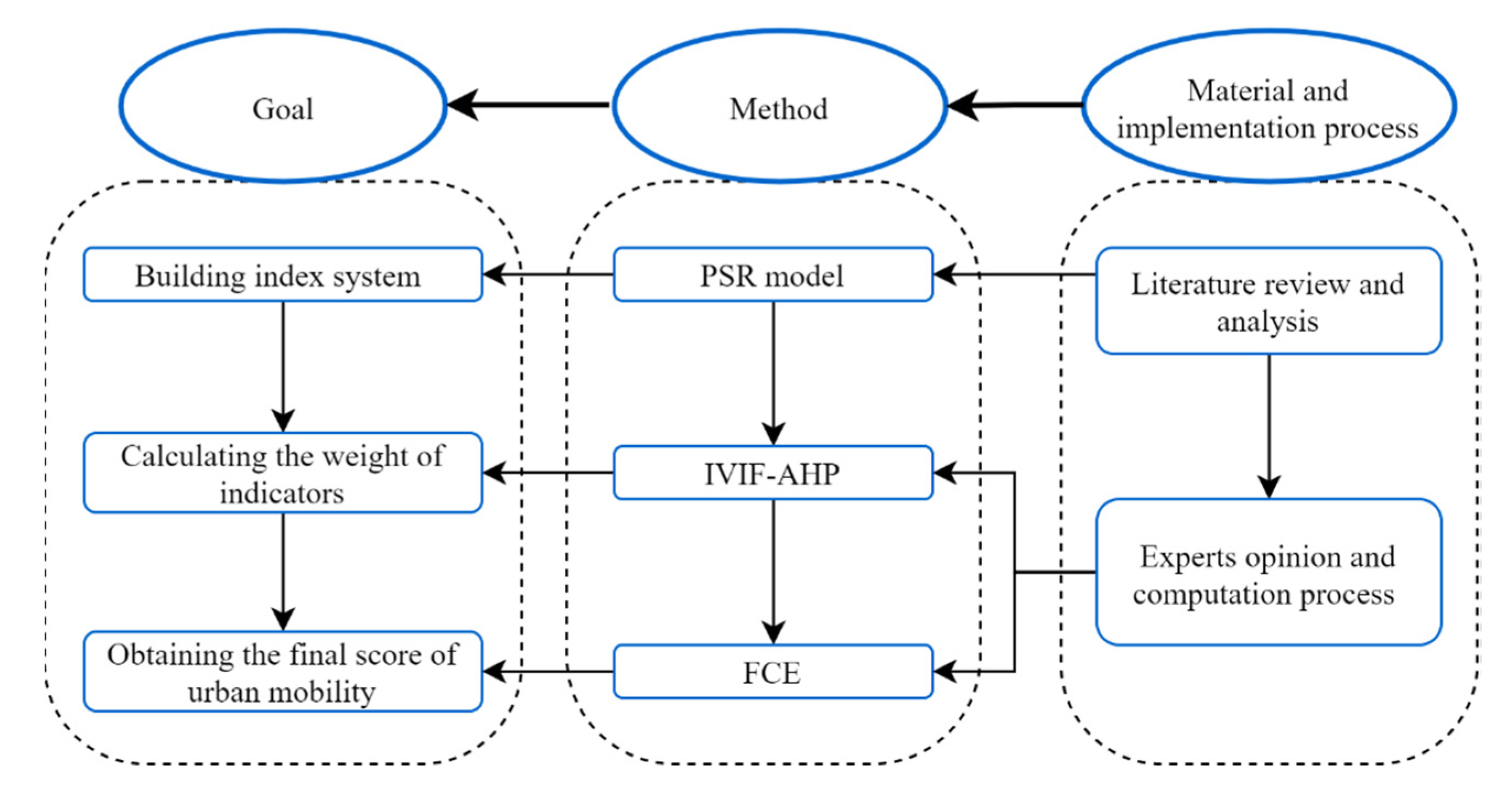
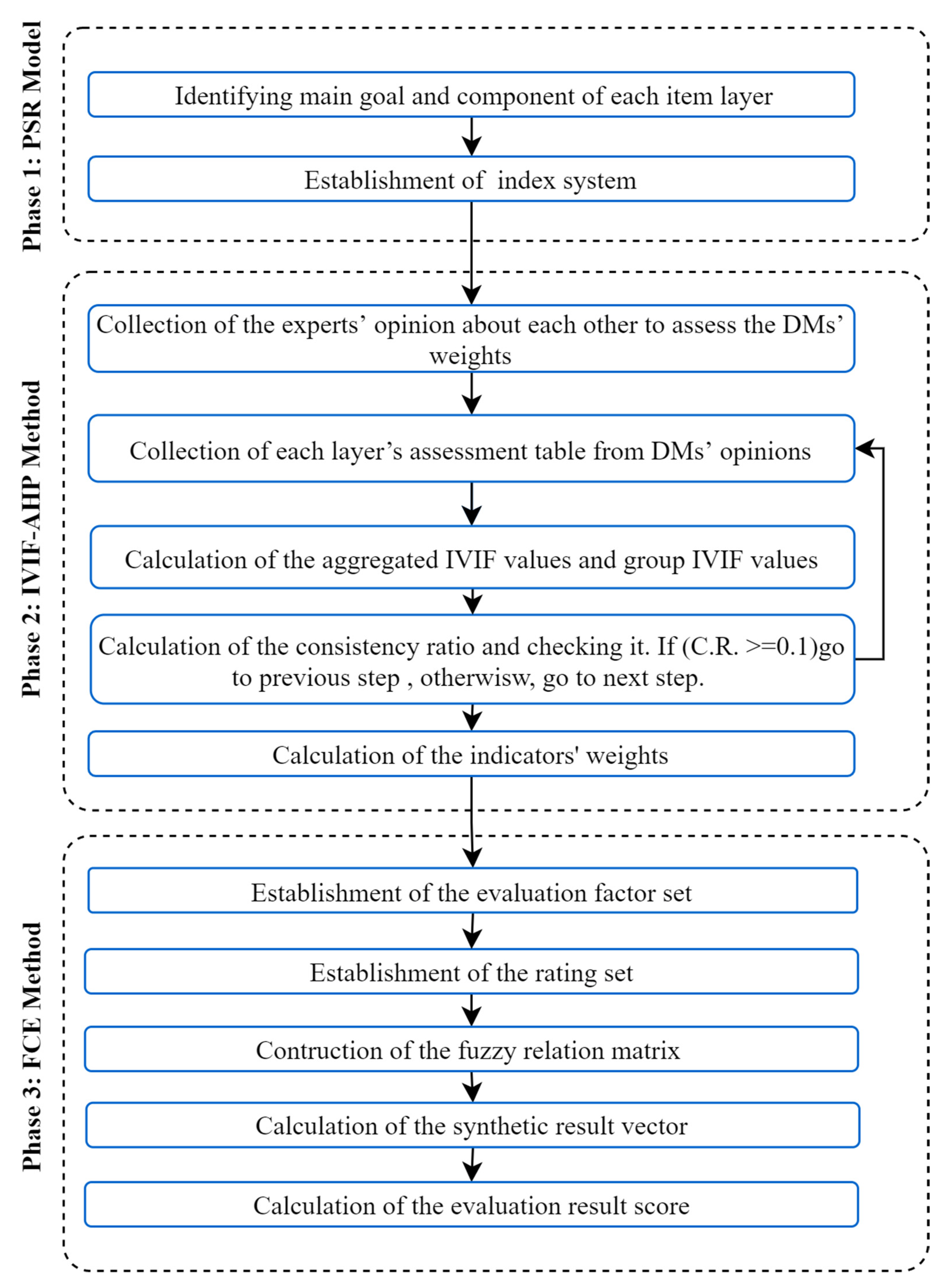
3. Methodology
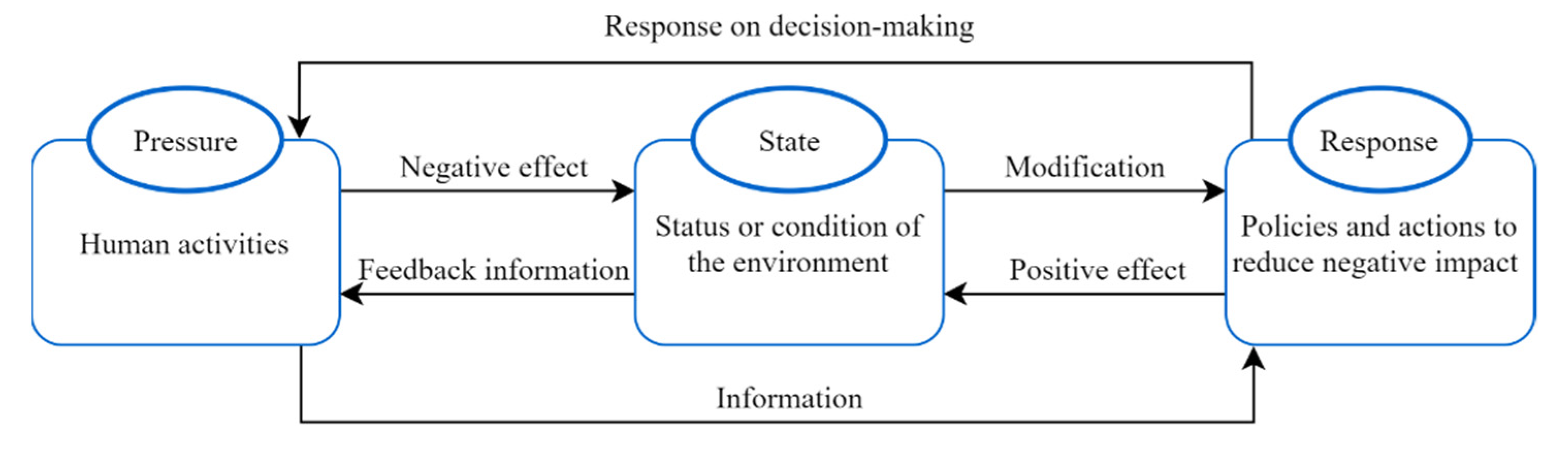
3.1. Establishment of an Index System with the PSR Model
3.2. Determination of Indicator Weights with IVIF-AHP
3.2.1. Preliminaries of IF and IVIF Sets
3.2.2. Calculation Procedure of the IVIF-AHP Method
3.3. Grade Evaluation with FCE
4. Case Study
4.1. Case Background
4.2. Implementation of the Proposed Model
5. Results and Discussion
5.1. IVIF-AHP Weight for Each Indicator
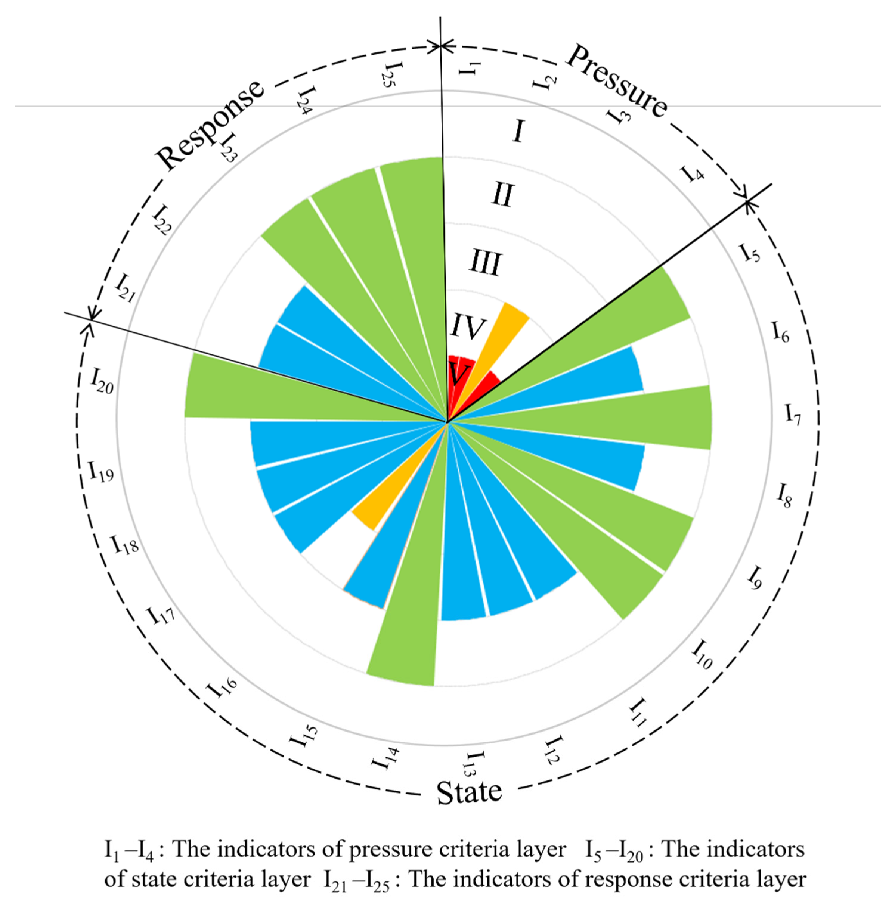
5.2. FCE Assessment Result
6. Conclusions
Author Contributions
Funding
Institutional Review Board Statement
Informed Consent Statement
Data Availability Statement
Conflicts of Interest
References
- Huan, Y. The Management of Current Traffic Congestion Status during the Urbanization Development in Guiyang. Stud. Sociol. Sci. 2011, 2, 23–28. [Google Scholar]
- Buhaug, H.; Urdal, H. An Urbanization Bomb? Population Growth and Social Disorder in Cities. Glob. Environ. Chang. 2013, 23, 1–10. [Google Scholar] [CrossRef]
- Al-Mulali, U.; Fereidouni, H.G.; Lee, J.Y.M.; Sab, C.N.B.C. Exploring the Relationship between Urbanization, Energy Consumption, and CO2 Emission in MENA Countries. Renew. Sustain. Energy Rev. 2013, 23, 107–112. [Google Scholar] [CrossRef]
- Liang, L.; Wang, Z.; Li, J. The Effect of Urbanization on Environmental Pollution in Rapidly Developing Urban Agglomerations. J. Clean. Prod. 2019, 237, 117649. [Google Scholar] [CrossRef]
- Wu, C.; Pei, Y.; Gao, J. Model for Estimation Urban Transportation Supply-Demand Ratio. Math. Probl. Eng. 2015, 2015, 1–12. [Google Scholar]
- Haghshenas, H.; Vaziri, M.; Gholamialam, A. Evaluation of Sustainable Policy in Urban Transportation Using System Dynamics and World Cities Data: A Case Study in Isfahan. Cities 2015, 45, 104–115. [Google Scholar] [CrossRef]
- Duarte, A.; Garcia, C.; Giannarakis, G.; Limão, S.; Polydoropoulou, A.; Litinas, N. New Approaches in Transportation Planning: Happiness and Transport Economics. NETNOMICS Econ. Res. Electron. Netw. 2009, 11, 5–32. [Google Scholar] [CrossRef] [Green Version]
- Sha, F.; Li, B.; Law, Y.W.; Yip, P.S.F. Associations between Commuting and Well-Being in the Context of a Compact City with a Well-Developed Public Transport System. J. Transp. Health 2019, 13, 103–114. [Google Scholar] [CrossRef]
- Yin, C.; Shao, C.; Dong, C.; Wang, X. Happiness in Urbanizing China: The Role of Commuting and Multi-Scale Built Environment across Urban Regions. Transp. Res. Part D Transp. Environ. 2019, 74, 306–317. [Google Scholar] [CrossRef]
- Yan-yan, C.; Pan-yi, W.; Jian-hui, L.; Guo-chen, F.; Xin, L.; Yi, G. An Evaluating Method of Public Transit Accessibility for Urban Areas Based on GIS. Procedia Eng. 2016, 137, 132–140. [Google Scholar] [CrossRef]
- Oses, U.; Rojí, E.; Cuadrado, J.; Larrauri, M. Multiple-Criteria Decision-Making Tool for Local Governments to Evaluate the Global and Local Sustainability of Transportation Systems in Urban Areas: Case Study. J. Urban Plan. Dev. 2018, 144, 04017019. [Google Scholar] [CrossRef]
- Tahanisaz, S.; Shokuhyar, S. Evaluation of Passenger Satisfaction with Service Quality: A Consecutive Method Applied to the Airline Industry. J. Air Transp. Manag. 2020, 83, 101764. [Google Scholar] [CrossRef]
- Li, Q.; Chen, Q.-Y.; Liu, Z.; Liu, H.-C. Public Transport Customer Satisfaction Evaluation Using an Extended Thermodynamic Method: A Case Study of Shanghai, China. Soft Comput. 2021, 25, 10901–10914. [Google Scholar] [CrossRef]
- Organization for Economic Co-Operation and Development (OECD). Core Set of Indicators for Environmental Performance. Paris, France, 1993; Available online: http://enrin.grida.no/ (accessed on 8 October 2021).
- Feng, Y.; Liu, Y.; Liu, Y. Spatially Explicit Assessment of Land Ecological Security with Spatial Variables and Logistic Regression Modeling in Shanghai, China. Stoch. Environ. Res. Risk Assess. 2016, 31, 2235–2249. [Google Scholar] [CrossRef]
- Men, B.; Liu, H. Water Resource System Vulnerability Assessment of the Heihe River Basin Based on Pressure-State-Response (PSR) Model under the Changing Environment. Water Supply 2018, 18, 1956–1967. [Google Scholar] [CrossRef]
- Das, S.; Pradhan, B.; Shit, P.K.; Alamri, A.M. Assessment of Wetland Ecosystem Health Using the Pressure-State-Response (PSR) Model: A Case Study of Mursidabad District of West Bengal (India). Sustainability 2020, 12, 5932. [Google Scholar] [CrossRef]
- Toloie-Eshlaghy, A.; Homayonfar, M. MCDM methodologies and applications: A literature review from 1999 to 2009. Res. J. Int. Stud. 2011, 21, 86–137. [Google Scholar]
- Chen, Y.-C.; Lien, H.-P.; Tzeng, G.-H. Measures and Evaluation for Environment Watershed Plans Using a Novel Hybrid MCDM Model. Expert Syst. Appl. 2010, 37, 926–938. [Google Scholar] [CrossRef]
- Teng, J.-Y.; Huang, W.-C.; Lin, M.-C. Systematic Budget Allocation for Transportation Construction Projects: A Case in Taiwan. Transportation 2009, 37, 331–361. [Google Scholar] [CrossRef]
- Alkharabsheh, A.; Duleba, S. Public Transportation Service Quality Evaluation during the COVID-19 Pandemic in Amman City Using Integrated Approach Fuzzy AHP-Kendall Model. Vehicles 2021, 3, 330–340. [Google Scholar] [CrossRef]
- Awasthi, A.; Chauhan, S.S.; Omrani, H. Application of Fuzzy TOPSIS in Evaluating Sustainable Transportation Systems. Expert Syst. Appl. 2011, 38, 12270–12280. [Google Scholar] [CrossRef]
- Ivanović, I.; Grujičić, D.; Macura, D.; Jović, J.; Bojović, N. One Approach for Road Transport Project Selection. Transp. Policy 2013, 25, 22–29. [Google Scholar] [CrossRef]
- Yucelgazi, F.; Yitmen, İ. An ANP Model for Risk Assessment in Large-Scale Transport Infrastructure Projects. Arab. J. Sci. Eng. 2018, 44, 4257–4275. [Google Scholar] [CrossRef]
- Celik, E.; Aydin, N.; Gumus, A.T. A Multiattribute Customer Satisfaction Evaluation Approach for Rail Transit Network: A Real Case Study for Istanbul, Turkey. Transp. Policy 2014, 36, 283–293. [Google Scholar] [CrossRef]
- Li, Y.; Zhao, L.; Suo, J. Comprehensive Assessment on Sustainable Development of Highway Transportation Capacity Based on Entropy Weight and TOPSIS. Sustainability 2014, 6, 4685–4693. [Google Scholar] [CrossRef] [Green Version]
- Kabir, G. Selection of Hazardous Industrial Waste Transportation Firm Using Extended VIKOR Method under Fuzzy Environment. Int. J. Data Anal. Tech. Strateg. 2015, 7, 40. [Google Scholar] [CrossRef]
- Nassereddine, M.; Eskandari, H. An Integrated MCDM Approach to Evaluate Public Transportation Systems in Tehran. Transp. Res. Part A Policy Pract. 2017, 106, 427–439. [Google Scholar] [CrossRef] [Green Version]
- Ghorbanzadeh, O.; Moslem, S.; Blaschke, T.; Duleba, S. Sustainable Urban Transport Planning Considering Different Stakeholder Groups by an Interval-AHP Decision Support Model. Sustainability 2018, 11, 9. [Google Scholar] [CrossRef] [Green Version]
- Hamurcu, M.; Eren, T. Strategic Planning Based on Sustainability for Urban Transportation: An Application to Decision-Making. Sustainability 2020, 12, 3589. [Google Scholar] [CrossRef]
- Moslem, S.; Campisi, T.; Szmelter-Jarosz, A.; Duleba, S.; Nahiduzzaman, K.M.; Tesoriere, G. Best–Worst Method for Modelling Mobility Choice after COVID-19: Evidence from Italy. Sustainability 2020, 12, 6824. [Google Scholar] [CrossRef]
- Guler, D.; Yomralioglu, T. Location Evaluation of Bicycle Sharing System Stations and Cycling Infrastructures with Best Worst Method Using GIS. Prof. Geogr. 2021, 73, 535–552. [Google Scholar] [CrossRef]
- Travisi, C.M.; Camagni, R.; Nijkamp, P. Impacts of Urban Sprawl and Commuting: A Modelling Study for Italy. J. Transp. Geogr. 2010, 18, 382–392. [Google Scholar] [CrossRef]
- Patterson, Z.; Saddier, S.; Rezaei, A.; Manaugh, K. Use of the Urban Core Index to Analyze Residential Mobility: The Case of Seniors in Canadian Metropolitan Regions. J. Transp. Geogr. 2014, 41, 116–125. [Google Scholar] [CrossRef]
- Moeinaddini, M.; Asadi-Shekari, Z.; Zaly Shah, M. An Urban Mobility Index for Evaluating and Reducing Private Motorized Trips. Measurement 2015, 63, 30–40. [Google Scholar] [CrossRef]
- Mendiola, L.; González, P.; Cebollada, À. The Relationship between Urban Development and the Environmental Impact Mobility: A Local Case Study. Land Use Policy 2015, 43, 119–128. [Google Scholar] [CrossRef]
- Hüging, H.; Glensor, K.; Lah, O. Need for a Holistic Assessment of Urban Mobility Measures—Review of Existing Methods and Design of a Simplified Approach. Transp. Res. Procedia 2014, 4, 3–13. [Google Scholar] [CrossRef] [Green Version]
- Regmi, M.B. Measuring Sustainability of Urban Mobility: A Pilot Study of Asian Cities. Case Stud. Transp. Policy 2020. [Google Scholar] [CrossRef]
- Šoštarić, M.; Vidović, K.; Jakovljević, M.; Lale, O. Data-Driven Methodology for Sustainable Urban Mobility Assessment and Improvement. Sustainability 2021, 13, 7162. [Google Scholar] [CrossRef]
- Saaty, T.L. A Scaling Method for Priorities in Hierarchical Structures. J. Math. Psychol. 1977, 15, 234–281. [Google Scholar] [CrossRef]
- Saaty, T.L. Decision Making with the Analytic Hierarchy Process. Int. J. Serv. Sci. 2008, 1, 83. [Google Scholar] [CrossRef] [Green Version]
- Javanbarg, M.B.; Scawthorn, C.; Kiyono, J.; Shahbodaghkhan, B. Fuzzy AHP-Based Multicriteria Decision Making Systems Using Particle Swarm Optimization. Expert Syst. Appl. 2012, 39, 960–966. [Google Scholar] [CrossRef]
- Goyal, T.; Kaushal, S. An Intelligent Scheduling Scheme for Real-Time Traffic Management Using Cooperative Game Theory and AHP-TOPSIS Methods for next Generation Telecommunication Networks. Expert Syst. Appl. 2017, 86, 125–134. [Google Scholar] [CrossRef]
- Moslem, S.; Duleba, S. Application of AHP for Evaluating Passenger Demand for Public Transport Improvements in Mersin, Turkey. Pollack Period. 2018, 13, 67–76. [Google Scholar] [CrossRef]
- Moslem, S.; Ghorbanzadeh, O.; Blaschke, T.; Duleba, S. Analysing Stakeholder Consensus for a Sustainable Transport Development Decision by the Fuzzy AHP and Interval AHP. Sustainability 2019, 11, 3271. [Google Scholar] [CrossRef] [Green Version]
- Moslem, S.; Alkharabsheh, A.; Ismael, K.; Duleba, S. An Integrated Decision Support Model for Evaluating Public Transport Quality. Appl. Sci. 2020, 10, 4158. [Google Scholar] [CrossRef]
- Mosadeghi, R.; Warnken, J.; Tomlinson, R.; Mirfenderesk, H. Comparison of Fuzzy-AHP and AHP in a Spatial Multi-Criteria Decision Making Model for Urban Land-Use Planning. Comput. Environ. Urban Syst. 2015, 49, 54–65. [Google Scholar] [CrossRef] [Green Version]
- Hamidy, N.; Alipur, H.; Nasab, S.N.H.; Yazdani, A.; Shojaei, S. Spatial Evaluation of Appropriate Areas to Collect Runoff Using Analytic Hierarchy Process (AHP) and Geographical Information System (GIS) (Case Study: The Catchment “Kasef” in Bardaskan. Model. Earth Syst. Environ. 2016, 2, 1–11. [Google Scholar] [CrossRef] [Green Version]
- Taylan, O.; Bafail, A.O.; Abdulaal, R.M.S.; Kabli, M.R. Construction Projects Selection and Risk Assessment by Fuzzy AHP and Fuzzy TOPSIS Methodologies. Appl. Soft Comput. 2014, 17, 105–116. [Google Scholar] [CrossRef]
- Lyu, H.-M.; Sun, W.-J.; Shen, S.-L.; Zhou, A.-N. Risk Assessment Using a New Consulting Process in Fuzzy AHP. J. Constr. Eng. Manag. 2020, 146, 04019112. [Google Scholar] [CrossRef]
- Fontoura, W.B.; Chaves, G.d.L.D.; Ribeiro, G.M. The Brazilian Urban Mobility Policy: The Impact in São Paulo Transport System Using System Dynamics. Transp. Policy 2019, 73, 51–61. [Google Scholar] [CrossRef]
- Mardani, A.; Zavadskas, E.K.; Khalifah, Z.; Jusoh, A.; Nor, K.M. Multiple Criteria Decision-Making Techniques in Transportation Systems: A Systematic Review of The State Of The Art Literature. Transport 2015, 31, 359–385. [Google Scholar] [CrossRef] [Green Version]
- Atanassov, K.T. Intuitionistic Fuzzy Sets. Fuzzy Sets Syst. 1986, 20, 87–96. [Google Scholar] [CrossRef]
- Mehdi, Z.; Mohammad, H.A.; Nahid, R.; Sarfaraz, H.Z. A Hybrid Fuzzy Multiple Criteria Decision Making (MCDM) Approach to Combination of Materials Selection. Afr. J. Bus. Manag. 2012, 6, 11171–11178. [Google Scholar] [CrossRef]
- Tumsekcali, E.; Ayyildiz, E.; Taskin, A. Interval Valued Intuitionistic Fuzzy AHP-WASPAS Based Public Transportation Service Quality Evaluation by a New Extension of SERVQUAL Model: P-SERVQUAL 4.0. Expert Syst. Appl. 2021, 186, 115757. [Google Scholar] [CrossRef]
- Seker, S.; Aydin, N. Sustainable Public Transportation System Evaluation: A Novel Two-Stage Hybrid Method Based on IVIF-AHP and CODAS. Int. J. Fuzzy Syst. 2020, 22, 257–272. [Google Scholar] [CrossRef]
- Dogan, O.; Deveci, M.; Canıtez, F.; Kahraman, C. A Corridor Selection for Locating Autonomous Vehicles Using an Interval-Valued Intuitionistic Fuzzy AHP and TOPSIS Method. Soft Comput. 2019, 24, 8937–8953. [Google Scholar] [CrossRef]
- Karaşan, A.; Kaya, İ.; Erdoğan, M. Location Selection of Electric Vehicles Charging Stations by Using a Fuzzy MCDM Method: A Case Study in Turkey. Neural Comput. Appl. 2018, 32, 4553–4574. [Google Scholar] [CrossRef]
- Liu, W.; Hui, L.; Lu, Y.; Tang, J. Developing an Evaluation Method for SCADA-Controlled Urban Gas Infrastructure Hierarchical Design Using Multi-Level Fuzzy Comprehensive Evaluation. Int. J. Crit. Infrastruct. Prot. 2020, 30, 100375. [Google Scholar] [CrossRef]
- Yang, Z.Y.; Wang, W.K.; Wang, Z.; Jiang, G.H.; Li, W.L. Ecology-Oriented Groundwater Resource Assessment in the Tuwei River Watershed, Shaanxi Province, China. Hydrogeol. J. 2016, 24, 1939–1952. [Google Scholar] [CrossRef]
- Zhang, D.; Yang, S.; Wang, Z.; Yang, C.; Chen, Y. Assessment of Ecological Environment Impact in Highway Construction Activities with Improved Group AHP-FCE Approach in China. Environ. Monit. Assess. 2020, 192. [Google Scholar] [CrossRef]
- Liu, Y.; Fang, P.; Bian, D.; Zhang, H.; Wang, S. Fuzzy Comprehensive Evaluation for the Motion Performance of Autonomous Underwater Vehicles. Ocean. Eng. 2014, 88, 568–577. [Google Scholar] [CrossRef]
- Yu, X.; Mu, C.; Zhang, D. Assessment of Land Reclamation Benefits in Mining Areas Using Fuzzy Comprehensive Evaluation. Sustainability 2020, 12, 2015. [Google Scholar] [CrossRef] [Green Version]
- Chuantao, W.; Xiaofei, C.; Baowen, L. Fuzzy Comprehensive Evaluation Based on Multi-Attribute Group Decision Making for Business Intelligence System. J. Intell. Fuzzy Syst. 2016, 31, 2203–2212. [Google Scholar] [CrossRef]
- Zhang, X.; Liu, H.; Xu, M.; Mao, C.; Shi, J.; Meng, G.; Wu, J. Evaluation of Passenger Satisfaction of Urban Multi-Mode Public Transport. PLoS ONE 2020, 15, e0241004. [Google Scholar] [CrossRef]
- Yang, J.; Sun, H.; Wang, L.; Li, L.; Wu, B. Vulnerability Evaluation of the Highway Transportation System against Meteorological Disasters. Procedia Soc. Behav. Sci. 2013, 96, 280–293. [Google Scholar] [CrossRef] [Green Version]
- Sun, J.; Liu, S.; Wang, L.; He, Z. Safety Resilience Evaluation of Urban Public Bus Based on Comprehensive Weighting Method and Fuzzy Comprehensive Evaluation Method. Available online: https://ieeexplore.ieee.org/abstract/document/9151734/ (accessed on 29 October 2021).
- Mihyeon Jeon, C.; Amekudzi, A. Addressing Sustainability in Transportation Systems: Definitions, Indicators, and Metrics. J. Infrastruct. Syst. 2005, 11, 31–50. [Google Scholar] [CrossRef]
- Solé-Ribalta, A.; Gómez, S.; Arenas, A. A Model to Identify Urban Traffic Congestion Hotspots in Complex Networks. R. Soc. Open Sci. 2016, 3, 160098. [Google Scholar] [CrossRef] [Green Version]
- Hao, H.; Wang, H.; Ouyang, M. Comparison of Policies on Vehicle Ownership and Use between Beijing and Shanghai and Their Impacts on Fuel Consumption by Passenger Vehicles. Energy Policy 2011, 39, 1016–1021. [Google Scholar] [CrossRef]
- Banister, D. Cities, Mobility and Climate Change. J. Transp. Geogr. 2011, 19, 1538–1546. [Google Scholar] [CrossRef]
- Ahmed, Q.I.; Lu, H.; Ye, S. Urban Transportation and Equity: A Case Study of Beijing and Karachi. Transp. Res. Part A Policy Pract. 2008, 42, 125–139. [Google Scholar] [CrossRef]
- Wong, R.C.P.; Szeto, W.Y.; Yang, L.; Li, Y.C.; Wong, S.C. Elderly Users’ Level of Satisfaction with Public Transport Services in a High-Density and Transit-Oriented City. J. Transp. Health 2017, 7, 209–217. [Google Scholar] [CrossRef] [Green Version]
- Hu, W.X.; Shalaby, A. Use of Automated Vehicle Location Data for Route- and Segment-Level Analyses of Bus Route Reliability and Speed. Transp. Res. Rec. J. Transp. Res. Board 2017, 2649, 9–19. [Google Scholar] [CrossRef]
- Jain, S.; Aggarwal, P.; Kumar, P.; Singhal, S.; Sharma, P. Identifying Public Preferences Using Multi-Criteria Decision Making for Assessing the Shift of Urban Commuters from Private to Public Transport: A Case Study of Delhi. Transp. Res. Part F Traffic Psychol. Behav. 2014, 24, 60–70. [Google Scholar] [CrossRef] [Green Version]
- Yaakub, N.; Napiah, M. Public transport: Punctuality index for bus operation. World Acad. Sci. Eng. Technol. 2011, 60, 857–862. [Google Scholar]
- Di Pasquale, G.; dos Santos, A.S.; Leal, A.G.; Tozzi, M. Innovative Public Transport in Europe, Asia and Latin America: A Survey of Recent Implementations. Transp. Res. Procedia 2016, 14, 3284–3293. [Google Scholar] [CrossRef] [Green Version]
- Chica-Olmo, J.; Gachs-Sánchez, H.; Lizarraga, C. Route Effect on the Perception of Public Transport Services Quality. Transp. Policy 2018, 67, 40–48. [Google Scholar] [CrossRef] [Green Version]
- Raha, U.; Taweesin, K. Encouraging the Use of Non-Motorized in Bangkok. Procedia Environ. Sci. 2013, 17, 444–451. [Google Scholar] [CrossRef] [Green Version]
- Kasemsuppakorn, P.; Karimi, H.A. A Pedestrian Network Construction Algorithm Based on Multiple GPS Traces. Transp. Res. Part C Emerg. Technol. 2013, 26, 285–300. [Google Scholar] [CrossRef]
- Szell, M.; Mimar, S.; Perlman, T.; Ghoshal, G.; Sinatra, R. Growing urban bicycle networks. arXiv 2021, arXiv:physics/2107.02185. [Google Scholar]
- Song, J.; Zhang, L.; Qin, Z.; Ramli, M.A. Where Are Public Bikes? The Decline of Dockless Bike-Sharing Supply in Singapore and Its Resulting Impact on Ridership Activities. Transp. Res. Part A Policy Pract. 2021, 146, 72–90. [Google Scholar] [CrossRef]
- Bai, Y.; Yu, X.; Chen, Y. Study on the Lateral Position Characteristics of Non-Motor Vehicles on the Urban Branch Roads. CICTP 2019, 2019, 3249–3261. [Google Scholar]
- Hitge, G.; Vanderschuren, M. Comparison of Travel Time between Private Car and Public Transport in Cape Town. J. S. Afr. Inst. Civ. Eng. 2015, 57, 35–43. [Google Scholar] [CrossRef]
- Chakrabarti, S. How Can Public Transit Get People out of Their Cars? An Analysis of Transit Mode Choice for Commute Trips in Los Angeles. Transp. Policy 2017, 54, 80–89. [Google Scholar] [CrossRef]
- Simićević, J.; Vukanović, S.; Milosavljević, N. The Effect of Parking Charges and Time Limit to Car Usage and Parking Behaviour. Transp. Policy 2013, 30, 125–131. [Google Scholar] [CrossRef]
- Berg, J.; Henriksson, M.; Ihlström, J. Comfort First! Vehicle-Sharing Systems in Urban Residential Areas: The Importance for Everyday Mobility and Reduction of Car Use among Pilot Users. Sustainability 2019, 11, 2521. [Google Scholar] [CrossRef] [Green Version]
- Nguyen-Phuoc, D.Q.; Su, D.N.; Tran, P.T.K.; Le, D.-T.T.; Johnson, L.W. Factors Influencing Customer’s Loyalty towards Ride-Hailing Taxi Services— A Case Study of Vietnam. Transp. Res. Part A Policy Pract. 2020, 134, 96–112. [Google Scholar] [CrossRef]
- Torrisi, V.; Ignaccolo, M.; Inturri, G. Innovative transport systems to promote sustainable mobility: Developing the model architecture of a traffic control and supervisor system. In International Conference on Computational Science and Its Applications; Springer: Cham, Germany, 2018; pp. 622–638. [Google Scholar]
- May, A.D. Encouraging Good Practice in the Development of Sustainable Urban Mobility Plans. Case Stud. Transp. Policy 2015, 3, 3–11. [Google Scholar] [CrossRef]
- Nikitas, A.; Michalakopoulou, K.; Njoya, E.T.; Karampatzakis, D. Artificial Intelligence, Transport and the Smart City: Definitions and Dimensions of a New Mobility Era. Sustainability 2020, 12, 2789. [Google Scholar] [CrossRef] [Green Version]
- Van Wee, B.; Maat, K.; De Bont, C. Improving Sustainability in Urban Areas: Discussing the Potential for Transforming Conventional Car-Based Travel into Electric Mobility. Eur. Plan. Stud. 2012, 20, 95–110. [Google Scholar] [CrossRef]
- Lyn, T.; Wang, P.; Gao, Y.; Wang, Y. Research on the Big Data of Traditional Taxi and Online Car-Hailing: A Systematic Review. J. Traffic Transp. Eng. 2021, 8, 1–34. [Google Scholar]
- Bustince Sola, H.; Burillo López, P. A Theorem for Constructing Interval-Valued Intuitionistic Fuzzy Sets from Intuitionistic Fuzzy Sets. Notes Intuit. Fuzzy Sets 1995, 1995, 5–16. [Google Scholar]
- Bustince, H.; Burillo, P. Correlation of Interval-Valued Intuitionistic Fuzzy Sets. Fuzzy Sets Syst. 1995, 74, 237–244. [Google Scholar] [CrossRef]
- Bustince, H.; Barrenechea, E.; Pagola, M.; Fernandez, J. Interval-Valued Fuzzy Sets Constructed from Matrices: Application to Edge Detection. Fuzzy Sets Syst. 2009, 160, 1819–1840. [Google Scholar] [CrossRef]
- Abdullah, L.; Najib, L. A New Preference Scale Mcdm Method Based on Interval-Valued Intuitionistic Fuzzy Sets and the Analytic Hierarchy Process. Soft Comput. 2014, 20, 511–523. [Google Scholar] [CrossRef]
- Xu, Z.; Cai, X. Intuitionistic Fuzzy Information Aggregation. In Intuitionistic Fuzzy Information Aggregation; Springer: Berlin/Heidelberg, Germany, 2012; pp. 1–102. [Google Scholar]
- Büyüközkan, G.; Göçer, F. An Extension of ARAS Methodology under Interval Valued Intuitionistic Fuzzy Environment for Digital Supply Chain. Appl. Soft Comput. 2018, 69, 634–654. [Google Scholar] [CrossRef]
- Oztaysi, B.; Onar, S.C.; Goztepe, K.; Kahraman, C. Evaluation of Research Proposals for Grant Funding Using Interval-Valued Intuitionistic Fuzzy Sets. Soft Comput. 2015, 21, 1203–1218. [Google Scholar] [CrossRef]
- National Bureau of Statistics. The China’s 6th National Census. Available online: http://www.stats.gov.cn/tjsj/pcsj/rkpc/6rp/indexch.htm (accessed on 10 October 2021).
- National Bureau of Statistics. The China’s 7th National Census. Available online: http://www.stats.gov.cn/ztjc/zdtjgz/zgrkpc/dqcrkpc/ (accessed on 10 October 2021).
- Beijing Bureau of Statistics. Beijing Statistical Yearbook. 2020. Available online: http://nj.tjj.beijing.gov.cn/nj/main/2020-tjnj/zk/indexch.htm (accessed on 11 October 2021).
- Beijing transport institute. Analysis on Commuting Characteristics and Typical Areas in Beijing. Available online: https://baijiahao.baidu.com/s?id=1643163807150154834&wfr=spider&for=pc (accessed on 11 October 2021).
- Beijing transport institute. 2021 Beijing Transport Development Annual Report. Available online: https://www.bjtrc.org.cn/List/index/cid/7.html (accessed on 11 October 2021).
- The People’s Government of Beijing Municipality. Action Plan of Beijing Traffic Management in 2019. Available online: http://www.gov.cn/xinwen/2019-04/09/content_5380930.htm (accessed on 11 October 2021).
- Beijing Municipal Commission of Development and Reform. Beijing’s 14th Five-Year Plan. Available online: http://fgw.beijing.gov.cn/gzdt/fgzs/mtbdx/bzwlxw/202101/t20210127_2234025.htm (accessed on 11 October 2021).
- Pan, H. Urban mobility in China. In Sustainable Approaches to Urban Transport; Institute for Mobility Research: Munich, Germany, 2019; p. 193. [Google Scholar]
- Tyfield, D.P.; Zuev, D.; Li, P.; Urry, J. The Politics and Practices of Low-Carbon Urban Mobility in China: 4 Future Scenarios. Available online: https://eprints.lancs.ac.uk/id/eprint/80292/1/Low_Carbon_China_Mobilities_Futures_Scenarios_CeMoRe_Report_Final.pdf (accessed on 11 October 2021).
- Zhang, Z.; Zhang, N. A Novel Development Scheme of Mobility as a Service: Can It Provide a Sustainable Environment for China? Sustainability 2021, 13, 4233. [Google Scholar] [CrossRef]
- Beijing Traffic Management Bureau. Available online: http://jtgl.beijing.gov.cn/jgj/jgxx/95495/ywsj/index.html (accessed on 11 October 2021).
- Zuev, D. Urban Mobility in Modern China: The Growth of the E-Bike; Springer: Cham, Germany, 2019. [Google Scholar]


| Techniques Used | Problem | Authors |
|---|---|---|
| Fuzzy AHP | Budget allocation for transportation infrastructure construction | Teng et al., 2009 [20] |
| Investigation of the pandemic’s impact on the quality of public transportation services | Alkharabsheh and Duleba, 2021 [21] | |
| Fuzzy TOSIS | Assessment of sustainable transport solutions | Awasthi et al., 2011 [22] |
| ANP | Selection of road transport projects | Ivanović et al., 2013 [23] |
| Risk assessment of large-scale transportation infrastructure | Yucelgazi and Yitmen, 2018 [24] | |
| VIKOR and interval type-2 fuzzy sets | Rail transit customer satisfaction assessment | Celik et al., 2014 [25] |
| Entropy and TOPSIS | Assessment of the sustainable development of the highway transportation capacity | Li et al., 2014 [26] |
| VIKOR with fuzzy set theory | Selection of hazardous industrial waste transportation firms | Kabir, 2015 [27] |
| Delphi ANP, GAHP and PROMETHEE | Assessment of public transport systems in Tehran | Nassereddine and Eskandari, 2017 [28] |
| IAHP | Sustainable urban transport planning considering different stakeholder groups | Ghorbanzadeh et al., 2018 [29] |
| AHP, Fuzzy TOPSIS | Suitable transport project selection for more urban livability | Hamurcu and Eren, 2020 [30] |
| Best worst method | Finding alternative mobility modes after COVID-19 | Moslem et al., 2020 [31] |
| Determining optimal locations of bicycle sharing system stations and cycling infrastructure | Guler and Yomralioglu, 2021 [32] |
| Criteria Layer | Factor Layer | Indicator Layer | Indicator Source |
|---|---|---|---|
| Pressure (C1) | The pressure of population growth (I1) | Solé-Ribalta et al., 2016 [69] | |
| The pressure of private vehicle ownership growth (I2) | Hao et al., 2011 [70] | ||
| The pressure of urban area growth (I3) | Banister, 2011 [71] | ||
| The pressure of an unreasonable urban structure (I4) | Ahmed et al., 2008 [72] | ||
| State (C2) | Public transport (F1) | Density level of public transport routes (I5) | Wong et al., 2017 [73] |
| Bus travel speed during peak hours (I6) | Hu and Shalaby, 2017 [74] | ||
| Social environment of giving preference to public transportation travel (I7) | Jain et al., 2014 [75] | ||
| Punctuality of public transport (I8) | Yaakub and Napiah, 2011 [76] | ||
| Connection performance between urban transit and other modes (I9) | Di et al., 2016 [77] | ||
| Density level of urban public transportation stations (I10) | Chica-Olmo et al., 2018 [78] | ||
| No-motorized traffic (F2) | Social environment of giving preference to non-motorized travel (I11) | Raha and Taweesin, 2013 [79] | |
| Pedestrian walkway setting level (I12) | Kasemsuppakorn and Karimi, 2013 [80] | ||
| Density level of the bicycle network (I13) | Szell et al., 2021 [81] | ||
| Supply and demand matching performance of shared bikes (I14) | Song et al., 2021 [82] | ||
| The partition between motor vehicles and non-motorized traffic (I15) | Bai and Chen, 2019 [83] | ||
| Personalized travel (F3) | Average travel speed of private vehicles during peak hours (I16) | Hitge and Vanderschuren, 2015 [84] | |
| Congestion duration level of private vehicles on weekdays (I17) | Chakrabarti, 2017 [85] | ||
| Supply capacity of parking spaces (I18) | Simićević et al., 2013 [86] | ||
| Convenience level of car rental (I19) | Berg et al., 2019 [87] | ||
| Average response speed of taxis and online car-hailing (I20) | Nguyen-Phuoc et al., 2020 [88] | ||
| Response (C3) | Improvement of urban traffic management (I21) | Torrisi et al., 2018 [89] | |
| Improvement of urban transport policy and regulations (I22) | May, 2015 [90] | ||
| Improvement of urban transport intelligence and informatization (I23) | Nikitas et al., 2020 [91] | ||
| The policy of supporting clean energy and new-energy vehicles (I24) | Van et al., 2012 [92] | ||
| Improvement of regulating and monitoring the service of taxis and online car-hailing (I25) | Lyn et al., 2021 [93] |
| Linguistic Variable | IVIF Values | ||
|---|---|---|---|
| Very qualified (VQ) | [0.95,1.00] | [0.00,0.00] | [0.00,0.05] |
| Qualified (Q) | [0.80,0.85] | [0.05,0.10] | [0.05,0.15] |
| Relatively qualified (RQ) | [0.60,0.65] | [0.10,0.15] | [0.20,0.30] |
| Relatively less qualified (RLQ) | [0.30,0.35] | [0.25,0.30] | [0.35,0.45] |
| Less qualified (LQ) | [0.20,0.25] | [0.30,0.35] | [0.40,0.50] |
| Very less qualified (VLQ) | [0.00,0.05] | [0.45,0.50] | [0.45,0.55] |
| Preference on Comparison | IVIF Values | Reciprocal IVIF Values |
|---|---|---|
| Equally important (EI) | [0.38,0.42], [0.22,0.58], [0,0.4] | [0.22,0.58], [0.38,0.42], [0,0.4] |
| Equally very important (EVI) | [0.29,0.41], [0.12,0.58], [0.01,0.59] | [0.12,0.58], [0.29,0.41], [0.01,0.59] |
| Moderately important (MI) | [0.10,0.43], [0.03,0.57], [0,0.87] | [0.03,0.57], [0.10,0.43], [0,0.87] |
| Moderately more important (MMI) | [0.03,0.47], [0.03,0.53], [0,0.94] | [0.03,0.53], [0.03,0.47], [0,0.94] |
| Strongly important (SI) | [0.13,0.53], [0.07,0.47], [0,0.8] | [0.07,0.47], [0.13,0.53], [0,0.8] |
| Strongly more important (SMI) | [0.32,0.62], [0.08,0.38], [0,0.6] | [0.08,0.38], [0.32,0.62], [0,0.6] |
| Very strongly more important (VSMI) | [0.52,0.72], [0.08,0.28], [0,0.4] | [0.08,0.28], [0.52,0.72], [0,0.4] |
| Extremely strong important (ESI) | [0.75,0.85], [0.05,0.15], [0,0.2] | [0.05,0.15], [0.75,0.85], [0,0.2] |
| Extremely more important (EMI) | [1,1], [0,0], [0,0] | [0,0], [1,1], [0,0] |
| n | 1–2 | 3 | 4 | 5 | 6 | 7 | 8 | 9 |
| RI | 0.0 | 0.58 | 0.90 | 1.12 | 1.24 | 1.32 | 1.41 | 1.45 |
| Evaluated Object | Evaluators | |||
|---|---|---|---|---|
| Expert1 | Expert2 | Expert3 | Expert4 | Expert5 |
| LQ | Q | Q | LQ | |
| Expert2 | Expert1 | Expert3 | Expert4 | Expert5 |
| Q | VQ | Q | VQ | |
| Expert3 | Expert1 | Expert2 | Expert4 | Expert5 |
| Q | LQ | Q | LQ | |
| Expert4 | Expert1 | Expert2 | Expert3 | Expert5 |
| VQ | RQ | Q | RQ | |
| Expert5 | Expert1 | Expert2 | Expert3 | Expert4 |
| Q | Q | Q | Q | |
| DM | ||||
|---|---|---|---|---|
| Expert1 | [0.600,0.665] | [0.122,0.187] | [0.148,0.278] | 0.182 |
| Expert2 | [0.900,1.000] | [0.000,0.000] | [0.000,0.100] | 0.219 |
| Expert3 | [0.600,0.665] | [0.122,0.187] | [0.148,0.278] | 0.182 |
| Expert4 | [0.800,1.000] | [0.000,0.000] | [0.000,0.200] | 0.208 |
| Expert5 | [0.800,0.850] | [0.050,0.100] | [0.050,0.150] | 0.209 |
| DM | Expert1 | Expert2 | Expert3 | Expert4 | Expert5 | |||||||||||||||
|---|---|---|---|---|---|---|---|---|---|---|---|---|---|---|---|---|---|---|---|---|
| Indicator | I1 | I2 | I3 | I4 | I1 | I2 | I3 | I4 | I1 | I2 | I3 | I4 | I1 | I2 | I3 | I4 | I1 | I2 | I3 | I4 |
| I1 | EI | EI | SI | SI | MI | EI | EI | SI | EI | EVI | ||||||||||
| I2 | SI | EI | EI | MI | SI | EI | SI | SI | MI | EI | MI | VSMI | EI | SMI | SI | |||||
| I3 | MI | EI | EI | EI | MI | EI | MI | EI | EI | |||||||||||
| I4 | SI | EI | SI | EI | EI | SI | EI | SI | EI | VSMI | SI | SI | EI | MI | SI | EI | ||||
| Indicators of Pressure | |||
|---|---|---|---|
| Expert1 | |||
| I1 | [0.1122,0.3836] | [0.2376,0.6164] | [0.0000,0.6503] |
| I2 | [0.1835,0.4244] | [0.3290,0.5756] | [0.0000,0.4875] |
| I3 | [0.1865,0.3404] | [0.2100,0.6596] | [0.0000,0.6035] |
| I4 | [0.2012,0.3769] | [0.2189,0.6231] | [0.0000,0.5799] |
| Expert2 | |||
| I1 | [0.1720,0.4362] | [0.1039,0.5638] | [0.0000,0.7241] |
| I2 | [0.1797,0.4353] | [0.1723,0.5647] | [0.0000,0.6480] |
| I3 | [0.1334,0.4413] | [0.1774,0.5587] | [0.0000,0.6893] |
| I4 | [0.2185,0.4450] | [0.1738,0.5550] | [0.0000,0.6077] |
| Expert3 | |||
| I1 | [0.1122,0.3836] | [0.2376,0.6164] | [0.0000,0.6503] |
| I2 | [0.1504,0.4003] | [0.1777,0.5997] | [0.0000,0.6718] |
| I3 | [0.1294,0.3425] | [0.1461,0.6575] | [0.0000,0.7245] |
| I4 | [0.1229,0.3969] | [0.2123,0.6031] | [0.0000,0.6649] |
| Expert4 | |||
| I1 | [0.1417,0.4035] | [0.2253,0.5965] | [0.0000,0.6330] |
| I2 | [0.1471,0.3821] | [0.1099,0.6179] | [0.0000,0.7430[ |
| I3 | [0.1277,0.4263] | [0.1920,0.5737] | [0.0000,0.6804] |
| I4 | [0.2677,0.5012] | [0.1414,0.4988] | [0.0000,0.5909] |
| Expert5 | |||
| I1 | [0.1766,0.3731] | [0.2539,0.6247] | [0.0022,0.5695] |
| I2 | [0.3032,0.5212] | [0.1468,0.4788] | [0.0000,0.5500] |
| I3 | [0.1465,0.4086] | [0.2912,0.5885] | [0.0030,0.5623] |
| I4 | [0.1525,0.4051] | [0.1324,0.5949] | [0.0000,0.7151] |
| Group IVIF value | |||
| I1 | [0.1449,0.3971] | [0.2092,0.6025] | [0.0005,0.6460] |
| I2 | [0.1941,0.4338] | [0.1835,0.5662] | [0.0000,0.6224] |
| I3 | [0.1439,0.3950] | [0.2044,0.6044] | [0.0006,0.6517] |
| I4 | [0.1944,0.4272] | [0.1736,0.5728] | [0.0000,0.6320] |
| Element of Each Layer | |||
|---|---|---|---|
| Criteria layer | |||
| C1 | [0.1116,0.2344] | [0.4880,0.7656] | [0.0000,0.4004] |
| C2 | [0.3460,0.4979] | [0.2568,0.5009] | [0.0012,0.3971] |
| C3 | [0.3902,0.4845] | [0.2261,0.5146] | [0.0009,0.3837] |
| Factor layer | |||
| F1 | [0.1725,0.3557] | [0.3181,0.6443] | [0.0000,0.5093] |
| F2 | [0.1504,0.3203] | [0.3006,0.6797] | [0.0000,0.5490] |
| F3 | [0.1477,0.2996] | [0.3288,0.7004] | [0.0000,0.5235] |
| Indicator layer (C1) | |||
| I1 | [0.1449,0.3971] | [0.2092,0.6025] | [0.0005,0.6460] |
| I2 | [0.1941,0.4338] | [0.1835,0.5662] | [0.0000,0.6224] |
| I3 | [0.1439,0.3950] | [0.2044,0.6044] | [0.0006,0.6517] |
| I4 | [0.1944,0.4272] | [0.1736,0.5728] | [0.0000,0.6320] |
| Indicator layer (C2-F1) | |||
| I5 | [0.1755,0.5950] | [0.1141,0.4032] | [0.0018,0.7104] |
| I6 | [0.2036,0.5285] | [0.0482,0.4711] | [0.0004,0.7482] |
| I7 | [0.1875,0.5436] | [0.0428,0.4559] | [0.0005,0.7698] |
| I8 | [0.2114,0.5474] | [0.0559,0.4524] | [0.0002,0.7327] |
| I9 | [0.1739,0.5587] | [0.0568,0.4412] | [0.0001,0.7693] |
| I10 | [0.1973,0.5563] | [0.0650,0.4433] | [0.0004,0.7377] |
| Indicator layer (C2-F2) | |||
| I11 | [0.1852,0.4948] | [0.0867,0.5052] | [0.0000,0.7281] |
| I12 | [0.1846,0.5031] | [0.1011,0.4969] | [0.0000,0.7144] |
| I13 | [0.1720,0.4718] | [0.0720,0.5282] | [0.0000,0.7560] |
| I14 | [0.1588,0.4888] | [0.1210,0.5112] | [0.0000,0.7202] |
| I15 | [0.1602,0.4837] | [0.1414,0.5163] | [0.0000,0.6984] |
| Indicator layer (C2-F3) | |||
| I16 | [0.1794,0.4715] | [0.0871,0.5285] | [0.0000,0.7336] |
| I17 | [0.1942,0.4778] | [0.0802,0.5222] | [0.0000,0.7256] |
| I18 | [0.1579,0.4884] | [0.1058,0.5116] | [0.0000,0.7363] |
| I19 | [0.1604,0.4938] | [0.1055,0.5062] | [0.0000,0.7342] |
| I20 | [0.1400,0.5029] | [0.1256,0.4971] | [0.0000,0.7344] |
| Indicator layer (C3) | |||
| I21 | [0.1603,0.4982] | [0.0988,0.5018] | [0.0000,0.7409] |
| I22 | [0.1908,0.4913] | [0.0951,0.5087] | [0.0000,0.7141] |
| I23 | [0.1674,0.4899] | [0.1026,0.5101] | [0.0000,0.7300] |
| I24 | [0.1543,0.4802] | [0.1064,0.5198] | [0.0000,0.7393] |
| I25 | [0.1495,0.4867] | [0.0820,0.5133] | [0.0000,0.7684] |
| Criteria Layer (Weight) | Factor Layer (Weight) | Indicator Layer | Weight | Global Weight |
|---|---|---|---|---|
| C1: Pressure (0.1507) | I1: The pressure of population growth | 0.2318 | 0.0349 | |
| I2: The pressure of private vehicle ownership growth | 0.2698 | 0.0407 | ||
| I3: The pressure of urban area growth | 0.2308 | 0.0348 | ||
| I4: The pressure of an unreasonable urban structure | 0.2674 | 0.0403 | ||
| C2: State (0.4196) | F1: Public transport (0.3685) | I5: Density level of public transport routes | 0.1701 | 0.0263 |
| I6: Bus travel speed during peak hours | 0.1639 | 0.0253 | ||
| I7: Social environment of giving preference to public transportation travel | 0.1644 | 0.0254 | ||
| I8: Punctuality of public transport | 0.1687 | 0.0261 | ||
| I9: Connection performance between urban transit and other modes | 0.1647 | 0.0255 | ||
| I10: Density level of urban public transportation stations | 0.1681 | 0.0260 | ||
| F2: Non-motorized travel (0.3272) | I11: Social environment of giving preference to non-motorized travel | 0.2059 | 0.0283 | |
| I12: Pedestrian walkway setting level | 0.2077 | 0.0285 | ||
| I13: Density level of the bicycle network | 0.1959 | 0.0269 | ||
| I14: Supply and demand matching performance of shared bikes | 0.1964 | 0.0270 | ||
| I15: The partition between motor vehicles and non-motorized traffic | 0.1942 | 0.0267 | ||
| F3: Personalized travel (0.3036) | I16: Average travel speed of private vehicles during peak hours | 0.1988 | 0.0253 | |
| I17: Congestion duration level of private vehicles on weekdays | 0.2046 | 0.0261 | ||
| I18: Supply capacity of parking spaces | 0.1983 | 0.0253 | ||
| I19: Convenience level of car rental | 0.2007 | 0.0256 | ||
| I20: Average response speed of taxis and online car-hailing | 0.1975 | 0.0252 | ||
| C3: Response (0.4292) | I21: Improvement of urban traffic management | 0.2017 | 0.0866 | |
| I22: Improvement of urban transport policy and regulations | 0.2070 | 0.0889 | ||
| I23: Improvement of urban transport intelligence and informatization | 0.2008 | 0.0862 | ||
| I24: The policy of supporting clean energy and new-energy vehicles | 0.1943 | 0.0834 | ||
| I25: Improvement of regulating and monitoring the service of taxis and online car-hailing | 0.1960 | 0.0841 |
| Grade | I | II | III | IV | V |
|---|---|---|---|---|---|
| Interval value | [0.8,1] | [0.6,0.8] | [0.4,0.6] | [0.2,0.4] | [0,0.2] |
| Score | 90 | 70 | 50 | 30 | 10 |
| Indicator | Grade |
|---|---|
| I1. The pressure of population growth | V |
| I2. The pressure of private vehicle ownership growth | V |
| I3. The pressure of urban area growth | IV |
| I4. The pressure of an unreasonable urban structure | V |
| I5. Density level of public transport routes | II |
| I6. Bus travel speed during peak hours | III |
| I7. Social environment of giving preference to public transportation travel | II |
| I8. Punctuality of public transport | III |
| I9. Connection performance between urban transit and other modes | II |
| I10. Density level of urban public transportation stations | II |
| I11. Social environment of giving preference to non-motorized travel | III |
| I12. Pedestrian walkway setting level | III |
| I13. Density level of the bicycle network | III |
| I14. Supply and demand matching performance of shared bikes | II |
| I15. The partition between motor vehicles and non-motorized traffic | III |
| I16. Average travel speed of private vehicles during peak hours | IV |
| I17. Congestion duration level of private vehicles on weekdays | III |
| I18. Supply capacity of parking spaces | III |
| I19. Convenience level of car rental | III |
| I20. Average response speed of taxis and online car-hailing | II |
| I21. Improvement of urban traffic management | III |
| I22. Improvement of urban transport policy and regulations | III |
| I23. Improvement of urban transport intelligence and informatization | II |
| I24.The policy of supporting clean energy and new-energy vehicles | II |
| I25. Improvement of regulating and monitoring service of the taxis and online car-hailing | II |
Publisher’s Note: MDPI stays neutral with regard to jurisdictional claims in published maps and institutional affiliations. |
© 2022 by the authors. Licensee MDPI, Basel, Switzerland. This article is an open access article distributed under the terms and conditions of the Creative Commons Attribution (CC BY) license (https://creativecommons.org/licenses/by/4.0/).
Share and Cite
Lu, X.; Lu, J.; Yang, X.; Chen, X. Assessment of Urban Mobility via a Pressure-State-Response (PSR) Model with the IVIF-AHP and FCE Methods: A Case Study of Beijing, China. Sustainability 2022, 14, 3112. https://doi.org/10.3390/su14053112
Lu X, Lu J, Yang X, Chen X. Assessment of Urban Mobility via a Pressure-State-Response (PSR) Model with the IVIF-AHP and FCE Methods: A Case Study of Beijing, China. Sustainability. 2022; 14(5):3112. https://doi.org/10.3390/su14053112
Chicago/Turabian StyleLu, Xi, Jiaqing Lu, Xinzheng Yang, and Xumei Chen. 2022. "Assessment of Urban Mobility via a Pressure-State-Response (PSR) Model with the IVIF-AHP and FCE Methods: A Case Study of Beijing, China" Sustainability 14, no. 5: 3112. https://doi.org/10.3390/su14053112