Calculation and Expression of the Urban Heat Island Indices Based on GeoSOT Grid

Abstract

The urban heat island (UHI) effect accelerates the accumulation of atmospheric pollutants, which has a strong impact on the climate of cities, circulation of material, and health of citizens. Therefore, it is of great significance to conduct quantitative monitoring and accurate governance of UHI by calculating the index rapidly and expressing spatial distribution accurately. In this paper, we proposed a model that integrates UHI information with the GeoSOT (Geographic Coordinate Subdividing Grid with One-Dimension Integer Coding on 2n Tree) grid and subsequently designed the calculation method of UHI indices and expression method of UHI spatial distribution. The UHI indices were calculated on Dongcheng and Xicheng District, Beijing, in the Summer of 2014 to 2019. Experimental results showed that the proposed method has higher calculation efficiency, and achieved a more detailed description of the spatial distribution of the urban thermal environment compared with the Gaussian surface fitting method. This method can be used for large-scale and high-frequency monitoring the level of UHI and expressing complicated spatial distribution of UHI inside the city, thus supporting accurate governance of UHI.

1. Introduction

Rapid urbanization has significantly increased the impervious surface of urban areas and affected the urban thermal cycle. At the same time, the population agglomeration, the growth of traffic volume, prosperous commercial activities, and industrial activities have thus caused the heat accumulation in urban areas, which leads to the urban heat island (UHI) effect [1,2]. This phenomenon has significantly influenced the climate, hydrology, material circulation, and energy metabolism of urban areas, and aggravated the accumulation of urban air pollutants, which adversely affect the lives and health of urban dwellers [3,4]. Therefore, it is of great significance to improve urban management and sustainable development by using quantitative monitoring and governing the urban heat island effect.

Traditional UHI monitoring methods use indices such as UHI intensity, UHI footprint, UHI capacity, and heat island proportion index to describe the level of the UHI, and the spatial distribution is usually expressed by the UHI intensity surface [5,6,7,8,9,10]. Streutker [11,12] fitted the Gaussian temperature surface to express the UHI intensity, UHI footprint, UHI centroid and visualized the temperature surface of Houston. The method was adopted by some urban heat island researches. Rajasekar [13] proposed a non-parametric model to compute the range, position, diffusion, and growth of UHI footprint. Tran [14] used the UHI signal function based on Gaussian fit to calculate the UHI capacity, then analyzed diurnal variations and seasonal variations. The radius method is used by Qiao [15] to identify the UHI footprint, calculate the UHI capacity and analyze the spatiotemporal variation characteristics. Zhan & Yang [16,17] used the supported vector machine method to calculate the UHI capacity and make a visual expression to the UHI intensity surface.

Since the thermal radiation energy of land surface targets can be detected by thermal infrared remote sensing technology, the remote sensing images are widely used to invert the UHI distribution of the land surface. With the development of satellite remote sensing technology in recent decades, abundant images with long time series, wide coverage, and high spatial resolution has been acquired to support monitoring of the urban thermal environment [18]. However, the large-scale and high-frequency calculation on both the UHI intensity and volume raises a higher requirement on efficiency, whereas the current functional models cannot support. On the other hand, previous studies mostly focus on the urban scale [19,20], and few dives inside the city to make a detailed UHI description. Moreover, the elaborate implications caused by the multi-scale urban spatial structure [21], building material [22], ventilation condition [23], and urban green index [24] result in multi-peak temperature surface, which is too complex to be represented by conventional surface fitting methods, thus the spatial distribution details of the thermal environment inside the city cannot be precisely described.

Discrete field model [25,26] has been proved to greatly improve the efficiency of spatial calculation and indexing by expressing certain unclear boundaries spatial objects or geographic phenomena that occupy continuous space by discrete spatial sampling. The rainfall process and pollution diffusion would be two good examples of applying this model. Therefore, the discrete field model is expected to solve the problems such as rapid calculation and detailed expression analysis of UHI indices. Common discrete field models include Regular grid cell, Regular grid point, Irregular divided point, Isoline, Irregular polygon, and Triangulated irregular network [27]. With the attention to global and regional large scene issues, the global subdivision grid has also received more and more attention in recent decades. A variety of subdivision modes have emerged, such as Cubed-Sphere Grid [28], Yin-Yang Grid [29], Adaptive-Mesh Refinement [30]. Among them, the global subdivision model based on GeoSOT (Geographic Coordinate Subdividing Grid with One-Dimension Integer Coding on 2n Tree) uniformly dissects geospatial into grid cells of different scales, identifies and expresses them according to the geospatial grid encoding rule, becomes a reference framework for meshing spatial data [31,32,33,34,35]. The Geospatial Grid Encoding Rule has been promulgated as the Chinese national standard [36], and it has been applied in different fields of data management and representation [37,38,39,40,41,42].

To address the problems of low efficiency of UHI indices calculation and imprecise in expressing complex spatial distribution of urban internal thermal environment, in this paper, we propose a model that integrates UHI information with GeoSOT grid, based on which an efficient calculation, analysis and expression method is designed for UHI indices and 3D UHI spatial distribution. By using the summer Landsat7/8 data from 2014 to 2019, evaluation and analysis are conducted on Dongcheng District and Xicheng District, Beijing, China, and the experimental results show that the proposed method has obvious advantages compared with the conventional method.

2. Study Area and Data Preprocessing

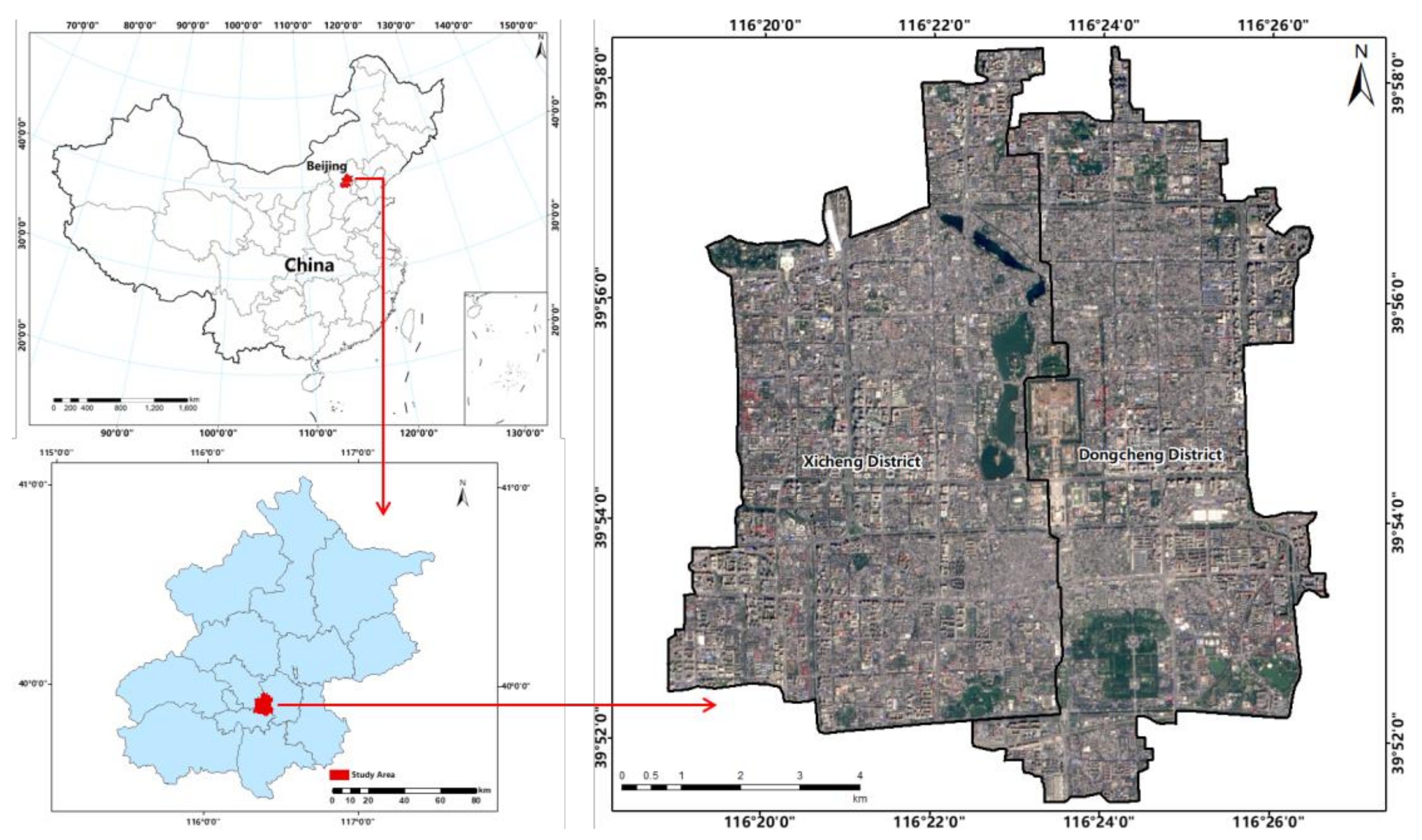
2.1. Study Area

As the core area of the capital of China [43], Dongcheng District and Xicheng District are the political, cultural, and international intercourse centers of the country, which occupies 92.49 km² of Beijing, as shown in Figure 1. Owing to the high aggregation of population, frequent commercial activities, high-density residential areas, and the significance of the UHI phenomenon, Dongcheng District and Xicheng District were selected to be the experimental area.

2.2. Land Surface Temperature (LST) Data Preprocessing

Landsat ETM+ and Landsat TIR images with no cloud cover were used to inverse the LST. The images of June, July, and August 2014–2019 were selected with the spatial resolution of 30 m (after spatial resampling). Subsequently, we fused the inversion results from June to August of each year to represent the LST for that summer.

The mono-window algorithm [44] was utilized to inverse the LST and obtained 125,780 points of LST for each year. Through the grid level selection method in Section 3.1, the 21st-level of GeoSOT grid with the size of 32 × 32 m was chosen, because the grid cell size of this level match well with the spatial resolution of LST points.

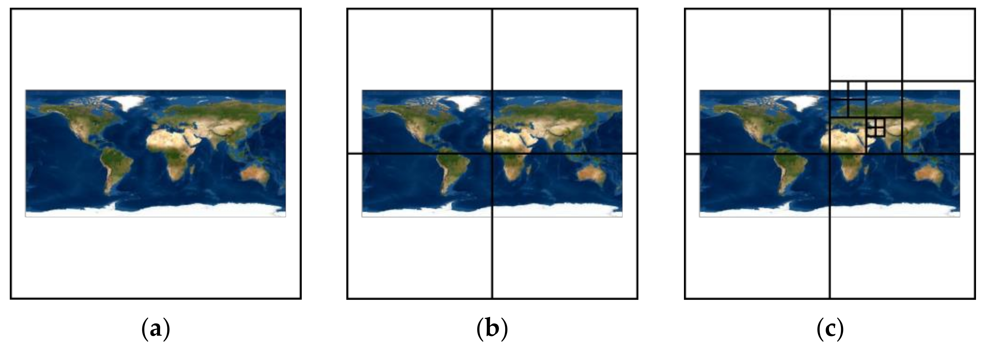
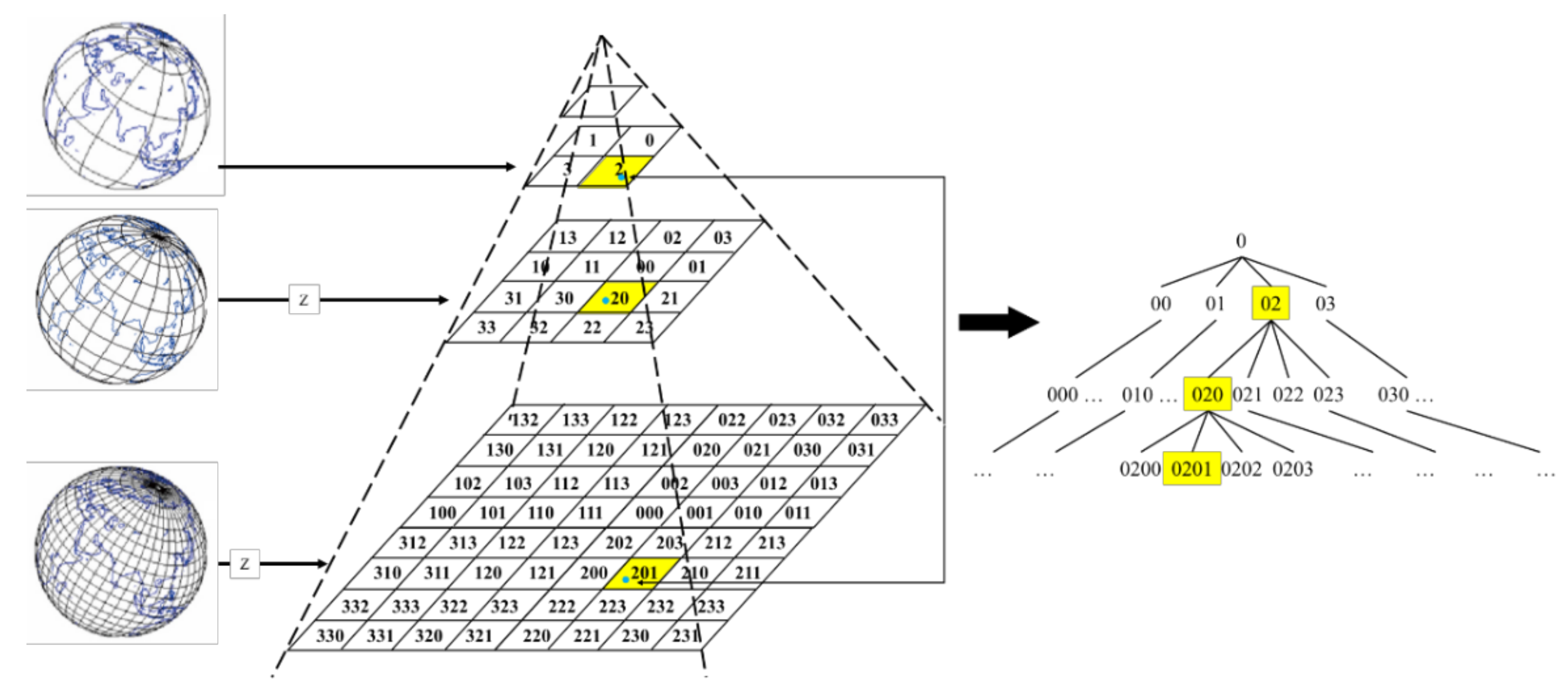
3. The UHI Information Model Based on GeoSOT Grid

Targeting at integrating UHI information with geospatial grids, two steps should be conducted, i.e., the determination of LST for grid cell, and the integration model of UHI information with GeoSOT grid.

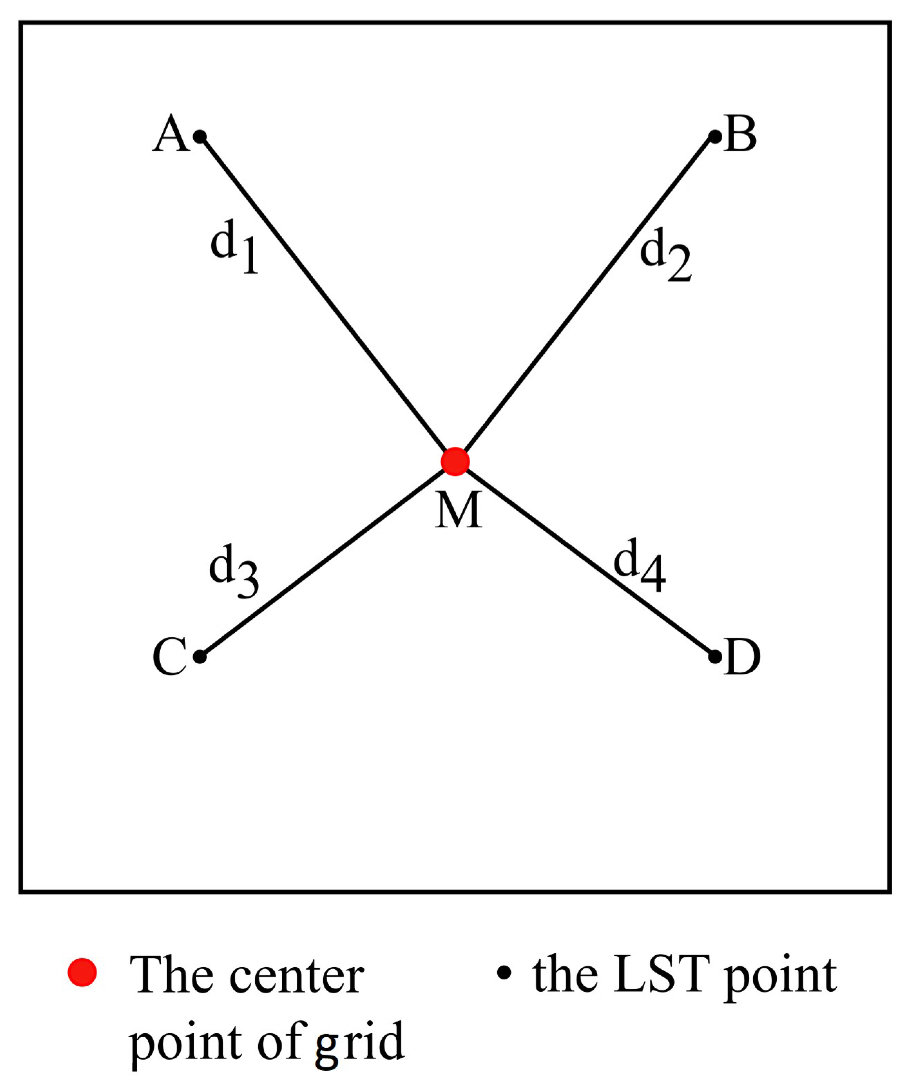
3.1. The Determination of LST for Grid Cell

GeoSOT subdivides the Earth into a 32-level multi-scale grid through quadtree recursive subdivision [45], the largest subdivision grid in the highest level (Level 0) can represent the entire Earth surface, while the smallest subdivision grid in the lowest level (Level 32). With the grid level corresponding to the grid scale. Each grid cell has a globally unique code by adopting the spatial Z-order coding method, as shown in Figure 2 and Figure 3.

The LST at the pixel center is obtained from the inversion of remote sensing images [44,46,47,48,49], which spatial resolution is consistent with the images used. The selected GeoSOT grid-level needs approximating to the spatial resolution of the images, for facilitating the calculation and ensuring the accuracy of calculation and expression of UHI indices. Therefore, the rules for grid-level selection are given by Equations (1) and (2).

Define the spatial resolution of the LST as δ, the total level of GeoSOT as K, n as a level in K. We have scale(n) as the grid size of the n level, and N is the recommended grid-level corresponding to the spatial resolution of the LST, then

$$if \delta =scale\left(n\right), n\in K, then N=n$$

(1)

$$if scale\left(n+1\right)<\delta <scale\left(n\right), n\in K, then N=n$$

(2)

There will be multiple LST points falling into the same grid when scale(N) is inconsistent with δ. In this paper, the LST that falls into the grid is calculated by the distance-weighted method, through which we can obtain the LST of the corresponding grid cell. The calculating Equations (3) and (4) and schematic (Figure 4) have shown in follows:

$$D_{SUM}=d_1+d_2+d_3+d_4$$

(3)

$$T_G=\frac{d_1}{D_{SUM}}{T}_A+\frac{d_2}{D_{SUM}}{T}_B+\frac{d_3}{D_{SUM}}{T}_C+\frac{d_4}{D_{SUM}}{T}_D$$

(4)

where M denotes the center point of grid G, and points A, B, C and D indicate the LST points falling into the grid G, respectively. $T_G$, $T_A$, $T_B$, $T_C$, $T_D$ represent the LST of point M, A, B, C, D. Specifically, $d_i$ is used to measure the distance from point A, B, C and D to point M.

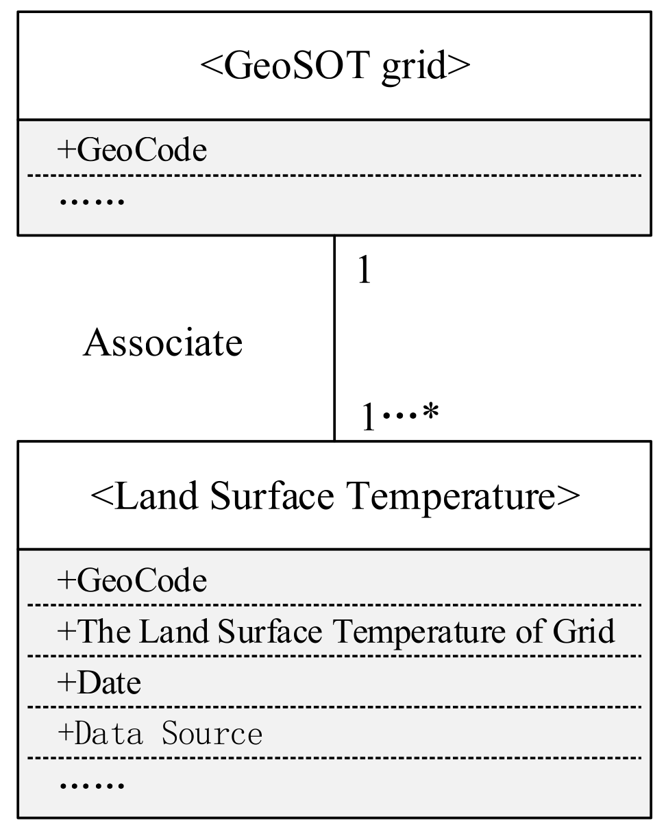
3.2. The Integration Model of UHI Information Based on GeoSOT Grid

The grid and LST association model is designed for the management and calculation of UHI information, as shown in Figure 5. GeoSOT code as the primary key in the model is used to achieve the correspondence between the gird and corresponding $T_G$ which calculate from the previous section. This association is a one-to-many relationship, i.e., a grid corresponds to multiple LST from different phases and different sources. Owing to the multi-level trait of the grid, the LST corresponding to the large-scale level grid are averaged from the LST of the grid at the level below it.

Table 1. The attribute table of the GeoSOT grid.

Field Name	Field Description	Constraint	Data Type
GeoCode-2D	the GeoSOT-2D grid codes	Primary Key	Varchar(30)

shows the grid data structure. As the primary key of the data Table, the GeoSOT code is used to identify the geospatial grid and correspond to the location and size of that grid, while recording the correlation information such as LST and sensors for each grid center data to provide support for UHI indices calculation and expression.

These attribute Tables are designed by the above model for the storage and management of data. Among them, Table 1 is the basic attribute Table of the GeoSOT grid, by decoding the grid code can obtain the position and size which are corresponding to the grid.

Table 2. The LST attribute table based on the GeoSOT grid.

Field Name	Field Description	Constraint	Data Type
GeoCode-2D	the GeoSOT-2D grid codes	Primary Key	Varchar(30)
Land Surface Temperature	The land surface temperature for grid center point		Double(8,6)
Date	Image date		DATE
Time	Image time		DATE
Data Source	Satellite ID		Varchar(10)

is the LST attribute table for each GeoSOT grid, mainly including LST, date, time, etc.

Table 3. The UHI indices attribute table based on the GeoSOT grid.

Field Name	Field Description	Constraint	Data Type
GeoCode-2D	the GeoSOT-2D grid codes	Primary Key	Varchar(30)
Date	Image date		DATE
Time	Image time		DATE
UHI Intensity	The urban heat island intensity for grid center point		Double(8,6)
UHI Footprint	The urban heat island footprint for grid center point		Double(8,6)
UHI capacity	The urban heat island capacity for grid center point		Double(10,6)

is an attribute Table of UHI indices, which is used to store the UHI indices calculated based on Table 2.

4. Calculation and Expression of the UHI Indices Based on GeoSOT Grid

4.1. Calculation of the UHI Intensity

UHI intensity is generally defined as the difference between the surface temperature in the urban center and the surface temperature in the countryside [50]. The study refers to the size-based method [51], where the area outside the urban boundary with the same area as the urban area is taken as the background temperature field region, and the average LST within this region is taken as the background temperature $T_{rural}$. Accordingly, the UHI intensity of grid G (UHII_G) is defined by the difference between the LST on gird ($T_G$) and $T_{rural}$:

$$UHI{I}_G=T_G-T_{rural}\hspace{1em}\hspace{1em}\hspace{1em}\hspace{1em}\hspace{1em}G=1,2\dots n$$

(5)

where the calculation of $T_{rural}$ is as follows:

$$T_{rural}={\displaystyle \sum }_{i=1}^k{T}_i/k$$

(6)

Among them, k is the number of LST in the region of the background temperature field.

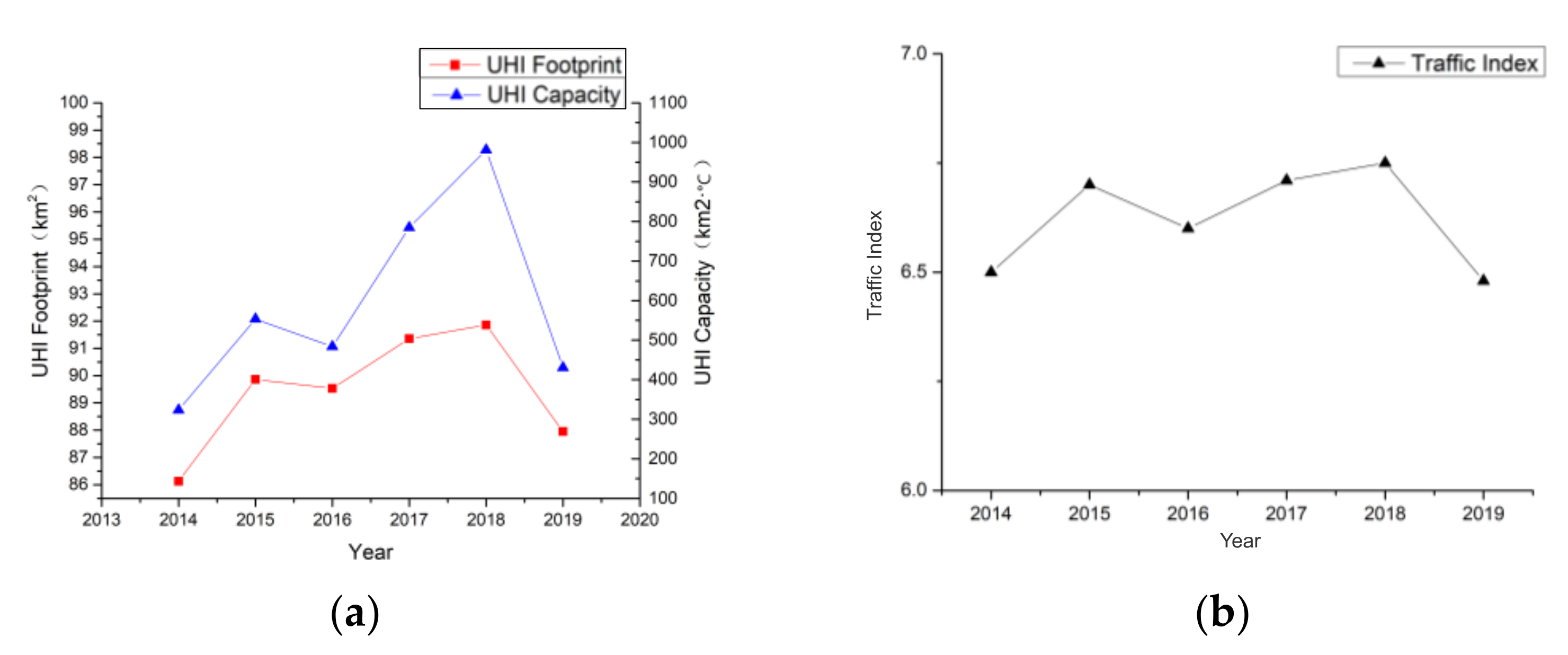
4.2. Calculation of the UHI Footprint

The UHI footprint is the area where the urban heat island effect is generated [15], the spatial extent at which the UHI effect occurs.

The area with UHI intensity greater than 0 is defined as the UHI footprint, then the UHI footprint is obtained by summarizing the area of the grids with UHI intensity greater than 0. The calculating equation is as follows:

$$F{P}_{SUM}={\displaystyle \sum }_{G=1}^{m}F{P}_G$$

(7)

where $F{P}_G$ is the UHI footprint of a grid cell i.e., the area of a grid cell, $F{P}_{SUM}$ is the total UHI footprint of the study area, and m is the number of grids in the study area with UHI intensity greater than 0.

4.3. Calculation of the UHI Capacity

The UHI capacity is the amount of UHI intensity accommodated within the UHI footprint and is the product of the UHI footprint and the UHI intensity [7,15]. It enables quantifying the significant degree for the occurrence of the UHI effect.

The UHI capacity $V_{UH{I}_G}$ for grid cell is calculated by using the UHI footprint $F{P}_G$ and the corresponding UHI intensity $UHI{I}_G$, then aggregated to the UHI capacity of the entire study area $V_{UH{I}_{SUM}}$, which is calculated as follows:

$$V_{UH{I}_G}=F{P}_G\times UHI{I}_G$$

(8)

$$V_{UH{I}_{SUM}}={\displaystyle \sum }_{i=1}^m{V}_{UH{I}_G}$$

(9)

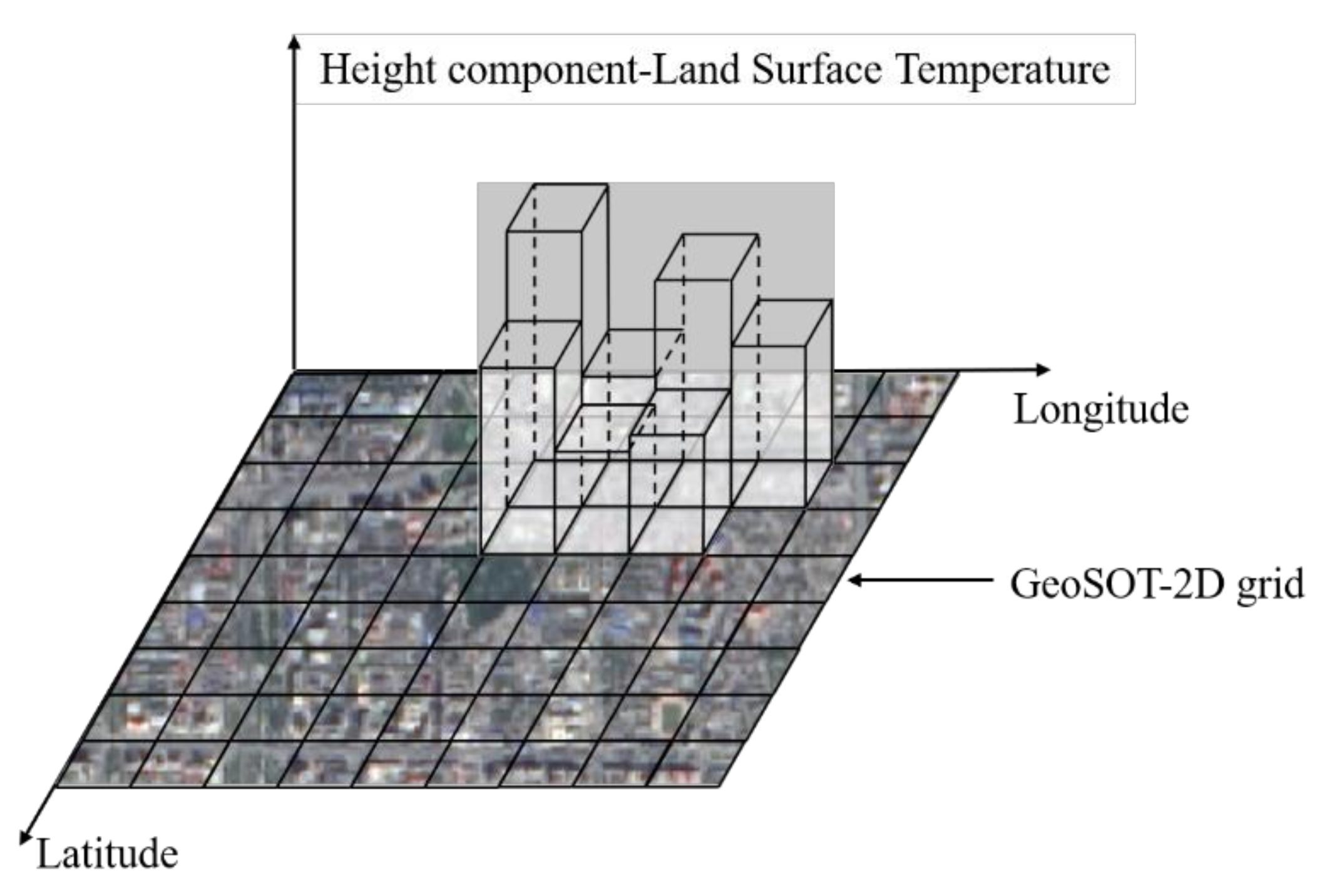
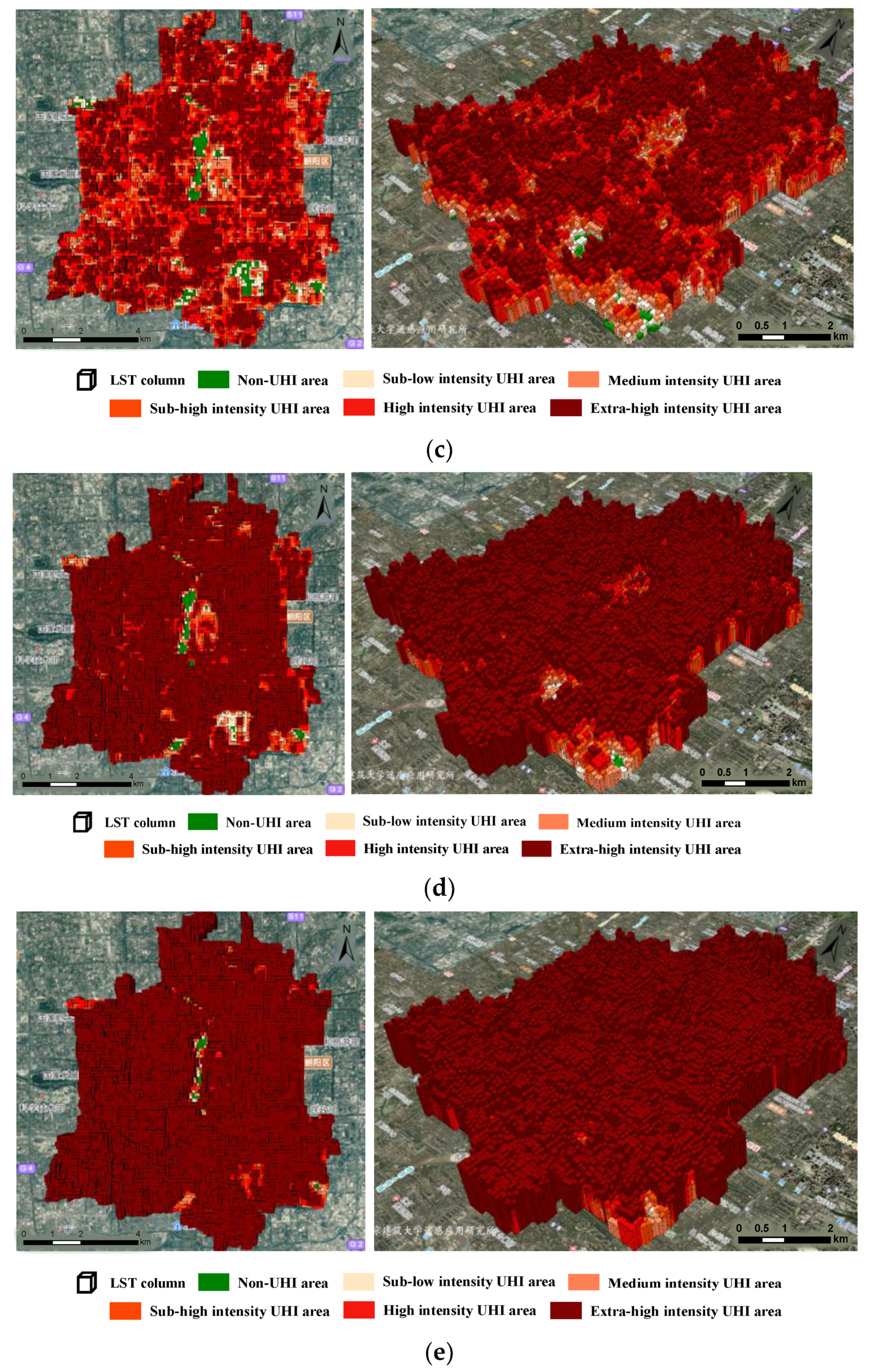
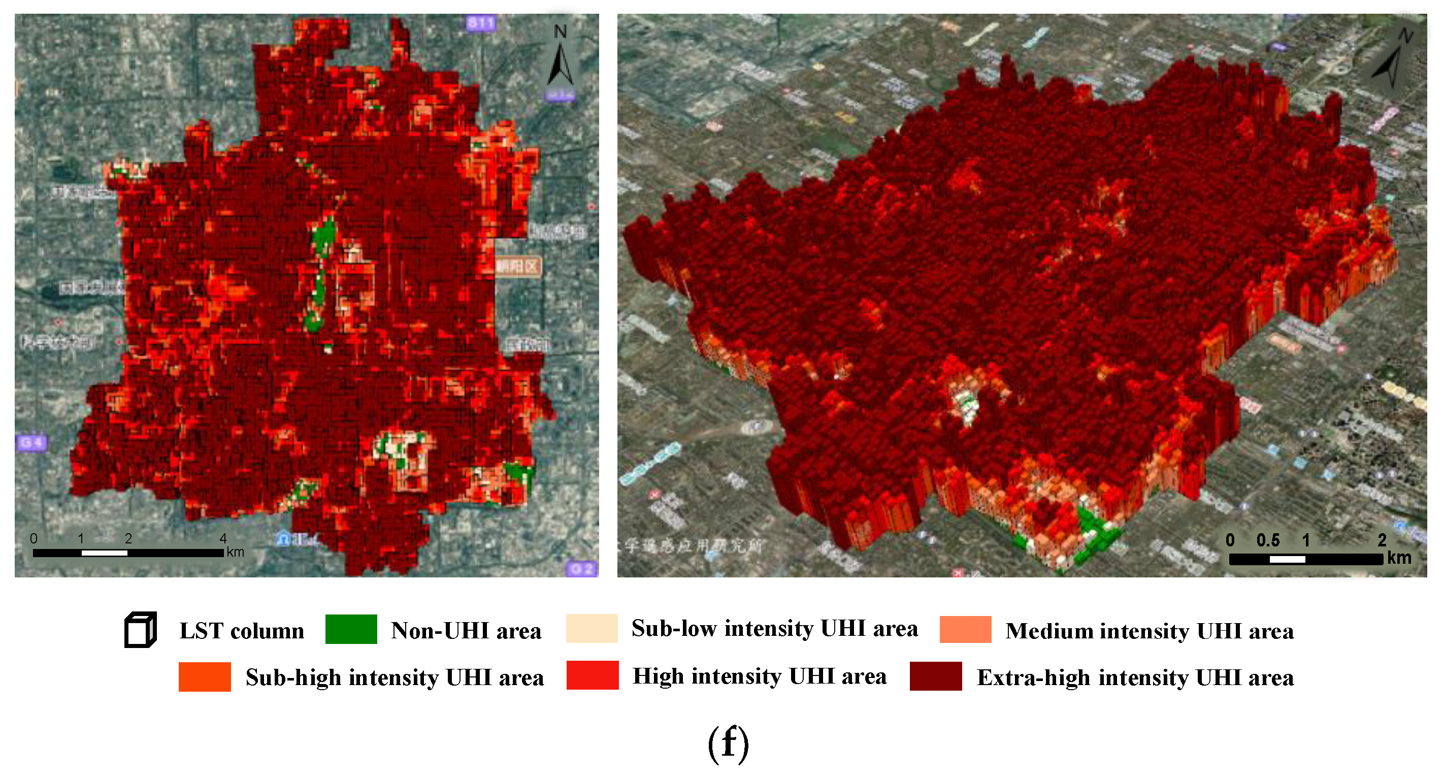
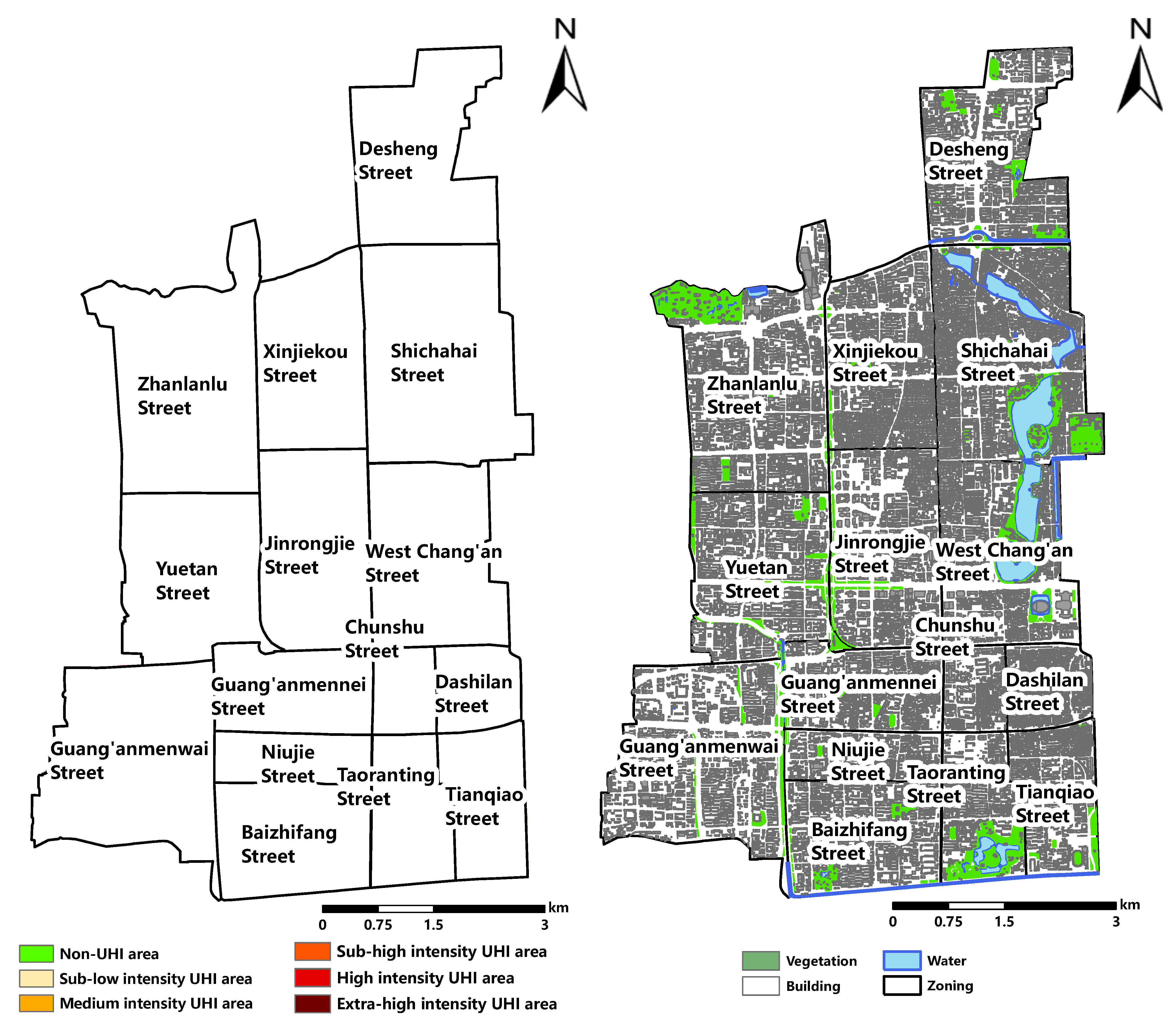
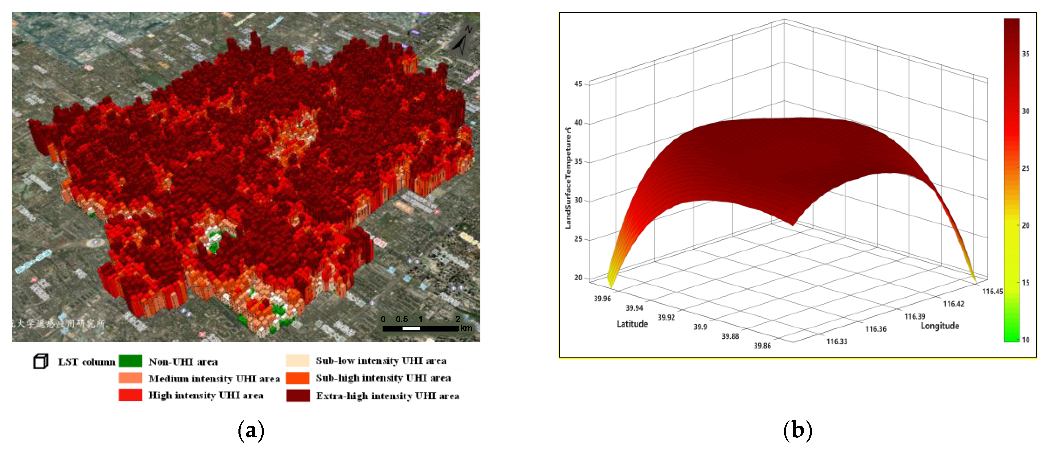
4.4. Expression of the UHI Spatial for Distribution Based on GeoSOT Grid

An expression method is proposed for the 3D spatial distribution of UHI using the discrete subdivision characteristic of the GeoSOT grid. Specifically, the LST of grid cells are set as height components, then constructing an LST column based on the 2D spatial distribution of the grid to portray the spatial distribution details of the urban thermal environment (as shown in Figure 6).

The expression of UHI intensity involves the classification of the UHI intensity category. Ge [52] used the quorum classification method to classify UHI as low intensity, sub-low intensity, medium intensity, sub-high intensity, and high intensity, then analyzed the spatial and temporal characteristics of UHI accordingly.

Due to the expression method can provide a more detailed description of UHI intensity, and to reflect the characteristics of its spatial distribution, this paper adds an extra-high intensity category based on Ge’s [52] UHI intensity category classification, as shown in

Table 4. UHI intensity classification.

UHI Intensity Zone	Division	UHI Intensity Levels
Non-UHI area	$UHI{I}_{P_i}\le 0 °\mathrm{C}$	0
Sub-low intensity UHI area	$0 °\mathrm{C}<UHI{I}_{P_i}\le 0.5 °\mathrm{C}$	1
Medium intensity UHI area	$0.5 °\mathrm{C}<UHI{I}_{P_i}\le 2.0 °\mathrm{C}$	2
Sub-high intensity UHI area	$2.0 °\mathrm{C}<UHI{I}_{P_i}\le 3.5 °\mathrm{C}$	3
High intensity UHI area	$3.5 °\mathrm{C}<UHI{I}_{P_i}\le 6.5 °\mathrm{C}$	4
Extra-high intensity UHI area	$UHI{I}_{P_i}>6.5 °\mathrm{C}$	5

.

5. Experiments Results and Analysis

5.1. Calculation of the Background Temperature

In this paper, we referred to the method proposed by li [53], employed the nighttime light data and the impervious surface data which proved to be valuable remote sensing data sources of detecting urban growth for extracting complete urban areas (Figure 7), among them, the nighttime light data was downloaded from NCEI National Centers for Environmental Information, and the impervious surface data was obtained from the team of Liu [54] named GLC_FCS-2015. Refers to the size-based method [51], where the buffer outside the urban boundary with the same area as the urban area was taken as the background temperature field region, and the background temperature of summer from 2014–2019 was calculated according to the method in Section 4.1, as shown in

Table 5. The background temperature of Beijing from 2014 to 2019.

Data	The Background Temperature
Summer of 2014	33.66 °C
Summer of 2015	34.37 °C
Summer of 2016	30.24 °C
Summer of 2017	34.35 °C
Summer of 2018	34.28 °C
Summer of 2019	35.04 °C

.

5.2. Calculation and Expression of the UHI Indices

UHI footprint and capacity in the summer of 2014–2019 were calculated and expressed by using the methods designed in Chapter 3. The calculation results and changing trend of UHI footprint and capacity were shown in

Table 6. The UHI parameters and rate of change in Beijing from 2014 to 2019 summer.

	Uhi Index	UHI Footprint (km2)	UHI Capacity (km2·°C)	The Growth Rate of UHI Footprint FPGR (km2/Year)	The Growth Rate of UHI Capacity CGR (km2·°C/Year)
Year
2014		86.13	323.21	-	-
2015		89.86	553.62	3.73	230.41
2016		89.53	483.77	−0.33	−69.85
2017		91.35	784.94	1.82	301.17
2018		91.86	980.85	0.51	195.91
2019		87.95	430.31	−3.91	−550.54

and Figure 8a respectively.

According to the result, both UHI footprint and capacity increased in stages, $F{P}_{GR}$ (the growth rate of UHI footprint) was 0.3 km²/year and $C_{GR}$ (the growth rate of capacity) was 17.85 km²·°C/year from 2014–2019. Among them, $F{P}_{GR}$ from 2014 to 2015 was the largest, which was 3.73 km²/year, and UHI capacity also increased by 230.41 km²· °C on this basis. From 2016 to 2017, $F{P}_{GR}$ and $C_{GR}$ were 1.82 km²/year and 301.17 km²· °C/year, respectively. Compared with the last period, under the condition of low $F{P}_{GR}$, $C_{GR}$ increased by about 70 km²· °C/year, it can be seen that UHI intensity changes the most during this period. The UHI footprint and capacity were increased by 0.51 km² and 195.91 km²·°C from 2017 to 2018, UHI intensity further strengthened and became the most significant year of the UHI effect in these six years. In 2019, the UHI effect was alleviated, and UHI footprint and capacity decreased by 3.91 km² and 550.54 km²·°C respectively.

Overall, the UHI effect in the experimental area gradually increased from 2014 to 2018. As the functional core area of the capital, the experimental area aggregate multiple urban functions which are driven to many problems such as increased traffic congestion [43], high building density and atmospheric pollution [55], these phenomena correspond to the influencing factors of UHI. In recent years, Beijing has formulated a series of measures, including improving the ventilation environment and reducing air pollution, to alleviate the urban heat island effect [56], which had achieved initial results at the end of 2018. According to the <2014–2019 Beijing Ecological Environment Status Bulletin> [57,58,59,60,61], the air quality and ecological environment index in 2019 were significantly improved compared with the previous year, among which PM_2.5, nitrogen dioxide (NO₂), inhalable particle (PM₁₀); it reached the national secondary standard for the first time, and the annual average concentration of sulfur dioxide (SO₂) reached single digits [61].This situation corresponds to the significant decrease in the UHI indices in 2019. Figure 8b shows the change of the traffic index during the same period, which is similar to the change trend of the UHI indices, it reflects the correlation between traffic congestion and the UHI effect to a certain extent.

Figure 9 shows the results of spatial distribution expression of UHI from 2014 to 2019. This expression method refined temperature fluctuations on each mesh, and more clearly expressed the details of the spatial and temporal distribution of UHI intensity inside the city.

The expression method in this paper can express the UHI intensity distribution not only in the entire study area but also in the designated area or street. The UHI indices of different streets in Xicheng District in 2015 were shown in

Table 7. The UHI indices of different streets in Xicheng District in 2015 summer.

	UHI Index	UHI Footprint (km2)	UHI Capacity (km2·°C)		UHI Index	UHI Footprint (km2)	UHI Capacity (km2·°C)
Street				Street
West Chang’an Street		3.58	21.49	Tianqiao Street		2.11	14.70
Xinjiekou Street		3.62	26.41	Chunshu Street		1.02	6.69
Yuetan Street		4.02	21.17	Taoranting Street		1.78	9.61
Zhanlanlu Street		5.53	34.22	Guang’anmennei Street		2.46	16.13
Desheng Street		3.97	23.84	Niujie Street		1.43	8.65
Jinrongjie Street		3.99	22.76	Baizhifang Street		3.10	18.34
Shichahai Street		5.17	35.85	Guang’anmenwai Street		5.37	29.39
Dashilan Street		1.28	12.78

. Among them, the UHI footprint in Dashilan Street accounts for 100%, and the extra-high intensity UHI area accounts for a large proportion. The UHI distribution information and the land cover vector diagram of the same area (Figure 10), it was shown that this block is a hutong residential area in the old city with high building density and low ventilation rate, which results in a high UHI intensity state in this area. Inversely, there is a park covering 0.57 km² in Taoranting street with the large water body [62] and vegetation [63] has a mitigating effect on the UHI effect in this area, thus the UHI footprint of this street has a relatively low percentage, and most of the areas are medium and sub-low intensity heat island state.

6. Comparison and Discussion

In this section, the proposed method is compared with the widely-used Gaussian surface fitting method [7,11,12] regarding the performance in calculation efficiency and UHI spatial distribution expression.

According to the Gaussian surface model [7,11], UHI$\left(x,y\right)$ is defined to be the LST increment caused by the UHI effect and obtained by fitting the key parameters in the Gaussian fit equation. Define the ellipse when U = 1 as the UHI footprint, and calculate it according to key parameters, then calculate the UHI capacity by the double integral method, finally fit the temperature surface by using the UHI$\left(x,y\right)$.

6.1. The Comparison of Calculation Efficiency

The GeoSOT grid method (the method proposed in this paper) and the Gaussian surface fitting method were utilized to calculate the UHI footprint and capacity, meanwhile, the point-by-point calculation result based on original inversion data was used to be the reference. The calculation results are shown in

Table 8. The calculation results of UHI footprint based on different methods from 2014 to 2019.

	UHI Footprint (km2)	The GeoSOT Grid Method	The Gaussian Surface Fitting Method	The Point-by-Point Method
Year
2014		86.13	92.49	85.75
2015		89.86	92.49	89.43
2016		89.53	92.49	89.14
2017		91.35	92.49	90.95
2018		91.86	92.49	91.46
2019		87.95	92.49	89.96

and

Table 9. The calculation results of UHI capacity based on different methods from 2014 to 2019.

	UHI Capacity (km2·°C)	The GeoSOT Grid Method	The Gaussian Surface Fitting Method	The Point-by-Point Method
Year
2014		323.21	325.33	321.84
2015		553.62	557.00	551.17
2016		483.77	489.74	481.44
2017		784.94	790.02	781.43
2018		980.85	979.88	976.48
2019		430.31	429.10	429.69

. The UHI indices calculation result shows the similar trend as those of previous researchers [64,65]. The errors of the Gaussian surface fitting method and the GeoSOT grid method are obtained respectively, using the point-by-point calculation result based on original inversion data as the true values (

Table 10. The errors and computing time of UHI indices.

Method	Data	The Average Error of UHI Footprint (km2)	The Average Error of UHI Capacity (km2·°C)	Average Time Cost (ms)
the point-by-point method	The UHI footprint, capacity from 2014 to 2019 summer	-	-	4952
the GeoSOT grid method	The UHI footprint, capacity from 2014 to 2019 summer	0.67	2.44	2569
the Gaussian surface fitting method	The UHI footprint, capacity from 2014 to 2019 summer	3.04	5.03	213

). Using the same device to perform calculations on the same data, the results demonstrate that the efficiency of the GeoSOT grid method is significantly improved when the accuracy in the similar level.

It should be noted that the calculation methods proposed in this paper depend on the resolution and quality of the remote sensing images. When the data is missing, there will be some difficulties in the calculation.

6.2. The Comparison of the UHI Spatial Distribution Expression

The grid method has even more significant advantages in the fine expression of the UHI spatial distribution. The spatial distributions of urban thermal environment in 2016 were expressed by the GeoSOT grid method and the Gaussian surface fitting method respectively, as shown in Figure 11a,b. The temperature surface fitted by the Gaussian model weakens the fluctuation of the LST, and can hardly reflect the spatial distribution characteristics of the thermal environment in the study area. While the GeoSOT grid method can reflect the fluctuations of the LST and the intensity distribution of the UHI visually and meticulously.

7. Conclusions

In this paper, we proposed a model that integrates UHI information with the GeoSOT grid, then designed the calculation method of UHI indices and expression method of UHI spatial distribution on this basis. Experimental results showed that compared with the Gaussian surface fitting method, the method proposed in this paper has higher efficiency of calculation, meanwhile, breaking the constraints of complex surface fitting and achieving the detailed description of the urban thermal environment spatial distribution by using the discrete subdivision way. The method supports a large range and high-frequency calculation of rapid calculation of UHI indices and accurate expression of spatial distribution, it is significant for accurate monitoring the changes of UHI, for analysis of connections between urban heat environment and complicated spatial distribution of cities, further to support accurate governance of UHI.

Future work will focus on the diversity of UHI spatial distribution, embedding multi-scale characteristics into the construction of multi-layer calculation models with GeoSOT grids, and solving limitations in data. Quantitative analysis of various influencing factors will also be applied, with the UHI information model based on the GeoSOT grid, among urban climate, urban distribution characteristics, urban spatial distribution, vegetation, and urban thermal environment.

References

1. Sun, Y.; Zhang, X.; Ren, G.; Zwiers, F.W.; Hu, T. Contribution of urbanization to warming in china. Nat. Clim. Chang. 2016, 6, 706. [Google Scholar] [CrossRef]
2. Huang, F.; Zhan, W.; Wang, Z.; Wang, K.; Chen, J.M.; Liu, Y.; Lai, J.; Ju, W. Positive or negative?Urbanization-induced variations in diurnal skin-surface temperature range detected using satellite data. J. Geophys. Res. Atmos. 2017, 122, 13229–13244. [Google Scholar] [CrossRef] [Green Version]
3. Sun, M.; Li, J. Analysis of Heat Island Effect of Urumqi Based on TM Remote Sensing Image Data. Bull. Surv. Mapp. 2015, 95–98. [Google Scholar]
4. Cui, Y.; Xu, X.; Dong, J.; Qin, Y. Influence of Urbanization Factors on Surface Urban Heat Island Intensity: A Comparison of Countries at Different Developmental Phases. Sustainability 2016, 8, 706. [Google Scholar] [CrossRef] [Green Version]
5. Yang, B.; Su, W.; Jang, N.; Zhen, F. Spatial-temporal characteristics of urban heat island effect change of Nanjing city and its relation with land use change. Geogr. Res. 2007, 26, 877–886. [Google Scholar]
6. Wang, Z. Study on Heat Island Effect Changes in Urban Agglomerations Based on Dense Time Series Analysis of Landsat; China University of Geosciences: Beijing, China, 2020. [Google Scholar]
7. Zhou, J.; Chen, Y.; Li, J.; Weng, Q.; Yi, W. A Volume Model for Urban Heat island Based on Remote Sensing Imagery and Its Application:A Case Study in Beijing. J. Remote Sens. 2008, 12, 734–742. [Google Scholar]
8. Ge, R. Impacts of urbanization on the urban thermal environment in Beijing. Acta Ecol. Sin. 2016, 36, 6040–6049. [Google Scholar]
9. Yang, Q.; Huang, X.; Tang, Q. The footprint of Urban Heat Island Effect in 302 Chinese Cities: Temporal Trends and Associated Factors. Sci. Total Environ. 2019, 655, 652–662. [Google Scholar] [CrossRef] [PubMed]
10. Liu, Y.; Fang, X.; Zhang, S.; Luan, Q.; Quan, W. Research on quantitative evaluations of heat islands for the Beijing-Tianjin-Hebei Urban Agglomeration. Acta Ecol. Sin. 2017, 37, 5818–5835. [Google Scholar]
11. Streutker, D.R. A Remote Sensing Study of the Urban Heat Island of Houston, Texas. Int. J. Remote Sens. 2002, 23, 2595–2608. [Google Scholar] [CrossRef]
12. Streutker, D.R. Satellite-Measured Growth of the Urban Heat Island of Houston, Texas. Remote Sens. Environ. 2003, 85, 282–289. [Google Scholar] [CrossRef]
13. Rajasekar, U.; Weng, Q. Spatio-Temporal modellingand analysis of urban heat islands by using Landsat TM and ETM+ imagery. Int. J. Remote Sens. 2009, 30, 3531–3548. [Google Scholar] [CrossRef]
14. Tran, H.; Uchiyama, D.; Ochi, S.; Yasuoka, Y. Assessment with satellite data of the urban heat island effects in Asian megacities. Int. J. Appl. Earth Obs. Geoinf. 2006, 8, 34–48. [Google Scholar] [CrossRef]
15. Qiao, Z.; Tian, G. Dynamic monitoring of the footprint and capacity for urban heat island in Beijing between 2001 and 2012 based on MODIS. Int. J. Remote Sens. 2015, 19, 476–484. [Google Scholar]
16. Zhan, W.; Chen, Y.; Zhou, J.; Li, J. Spatial Simulation of Urban Heat Island Intensity Based on the Support Vector Machine Technique: A Case Study in Beijing. Acta Geod. Cartogr. Sin. 2011, 40, 96–103. [Google Scholar]
17. Yang, H.; Meng, N.; Wang, Q.; Zheng, Y.; Zhao, L. Special-temporal Morphology Simulation of Beijing-Tianjin-Hebei Urban Agglomeration Thermal Environment based on Support Vector Machine. J. Geo-Inf. Sci. 2019, 21, 58–68. [Google Scholar]
18. Gao, Y.; Chang, M.; Zhao, J. Research on temporal and spatial variation of heat Island effect in Xi’an, China. Appl. Ecol. Environ. Res. 2019, 17, 231–244. [Google Scholar] [CrossRef]
19. Zhu, S.; Zhang, G.; Jian, C. Study on urban heat island of Shanghai by using multi-temporal remote sensing data and air temperature data. In Proceedings of the Urban Remote Sensing Event, Shanghai, China, 20–22 May 2009. [Google Scholar]
20. Annabelle, R.; Bonafoni, S.; Pichierri, M. Spatial and Temporal Trends of the Surface and Air Heat Island over Milan Using MODIS Data. Remote Sens. Environ. 2014, 150, 163–171. [Google Scholar] [CrossRef]
21. Gong, A.; Chen, Y.; Li, J.; Hu, L. Study on Relationship between Urban Heat Island and Urban Land Use and Cover Change in Beijing. J. Image Graph. 2007, 12, 1476–1482. [Google Scholar]
22. Kandya, A.; Mohan, M. Mitigating the Urban Heat Island Effect through Building Envelope Modifications. Energy Build. 2018, 164, 266–277. [Google Scholar] [CrossRef]
23. Liu, Y.; Xu, Y.; Zhang, F.; Shu, W. Influence of Beijing spatial morphology on the distribution of urban heat island. Acta Geogr. Sin. 2021, 76, 18. [Google Scholar]
24. Di, S.; Wu, W.; Liu, H.; Yang, S.; Pan, X. The Correlationship between Urban Greenness and Heat Island Effect with RS Technology: A Case Study with 5th Ring Road in Beijing. J. Geo-Inf. Sci. 2012, 14, 481–489. [Google Scholar]
25. Huang, F.; Fang, Y.; Chen, B.; Peng, X.; Yin, S. Continuous and Discrete Dynamic FieldsIntegrated Model and ItsDatabase Extension. Acta Sci. Nat. Univ. Pekin. 2007, 43, 9–14. [Google Scholar]
26. Tong, X. The Principles and Methods of Discrete Global Grid Systems for Geospatial Information Subdivision Organization. Acta Geod. Cartogr. Sin. 2011, 40, 1. [Google Scholar]
27. Cova, T.J.; Goodchild, M.F. Extending geographical representation to include fields of spatial objects. Int. J. Geogr. Inf. Sci. 2002, 16, 509–532. [Google Scholar] [CrossRef]
28. Choblet, G. Modelling convection with large viscosity gradients in the cubed sphere. Science 2005, 205, 269–291. [Google Scholar]
29. Kageyama, A. Dissection of a Sphere and Yin-Yang Grids. J. Earth Simulator 2005, 3, 20–28. [Google Scholar]
30. Stadler, G.; Gurnis, M.; Burstedde, C.; Wilcox, L.C.; Alisic, L.; Ghattas, O. The Dynamics of Plate Tectonics and Mantle Flow: From Local to Global Scales. Science 2010, 329, 1033–1038. [Google Scholar] [CrossRef]
31. Chen, C. Introduction to the Organization of Spatial Information Segmentation; Science Press: Beijing, China, 2012. [Google Scholar]
32. Lu, X.; Liao, Y.; Chen, C.; Jin, A. Multi-Source Remote Sensing Data Organization Based on GeoSOT Location Identification. Acta Sci. Nat. Univ. Pekin. 2014, 50, 331–340. [Google Scholar]
33. Sun, Z. Research on Ture-3D Subdivision Data Model; Peking University: Beijing, China, 2016. [Google Scholar]
34. Hu, X.; Chen, C.; Tong, X. The Representation of Three-Dimensional Data Based on GeoSOT-3D. Acta Sci. Nat. Univ. Pekin. 2015, 51, 1022–1028. [Google Scholar]
35. Deng, Q.; Guo, S.; Chen, C.; Pu, G. A method of spatial association for multi-sources remote sensing data based on global subdivision grid. Sci. Surv. Mapp. 2015, 40, 4. [Google Scholar]
36. National Standardization Administration. The Geospatial Grid Encoding Rule; GB/T 40087-2021; National Standardization Administration: Beijing, China, 2021.
37. Chen, R. Research on Location Coding Model of Meteorological Information Based on GeoSOT Subdivision Framework; Peking University: Beijing, China, 2012. [Google Scholar]
38. Guo, X. Research on the Relational Model of Subdivided Grid for Disaster Mitigation Data; Peking University: Beijing, China, 2013. [Google Scholar]
39. Liao, Y.; Li, B.; Lu, X.; Chen, C. Method of Multi-type Disaster Data Organization and Management Based on GeoSOT. Geogr. Geo-Inf. Sci. 2013, 29, 36–40. [Google Scholar]
40. Xin, H. Research on the Partition Coding Model of Spatial Information Location Markings: Taking the Monitoring Data of Geographic National Conditions as an Example; Peking University: Beijing, China, 2014. [Google Scholar]
41. Song, S.; Chen, C.; Pu, G.; An, F.; Luo, X. Global Remote Sensing Data Subdivision Organization Based on GeoSOT. Acta Geod. Cartogr. Sin. 2014, 43, 869–876. [Google Scholar]
42. Chen, C.; Chen, D.; Tong, X. The UAV Data Organization Model Based on Global Subdivision Grid. Geomat. World 2015, 22, 46–50. [Google Scholar]
43. Controlling Detailed Planning of the Capital Core Area (Block Level) (2018–2035). 2018. Available online: http://www.beijing.gov.cn/zhengce/zhengcefagui/202008/t20200828_1992592.html (accessed on 20 November 2021).
44. Tan, Z.; Li, W.; Zhang, M.; Karnieli, A.; Berliner, P. Estimating of The Essential Atmospheric Parameters of Mono-Window Algorithm for Land Surface Temperature Retrieval From Landsat TM6. Remote Sens. Nat. Resour. 2003, 15, 37–43. [Google Scholar]
45. Li, S.; Cheng, C.; Chen, B.; Meng, L. Integration and management of massive remote-sensing data based on GeoSOT subdivision model. J. Appl. Remote Sens. 2016, 10, 034003. [Google Scholar] [CrossRef]
46. Jiang, D.; Kuang, H.; Cao, X.; Huang, Y.; Li, F. Study of Land Surface Temperature Retrieval based on Landsat 8—With the Sample of Dianchi Lake Basin. Remote Sens. Technol. Appl. 2015, 30, 448–454. [Google Scholar]
47. Wang, Q.; Tan, Z.; Wang, F. Mono-window Algorithm for Retrieving Land Surface Temperature Based on Multi-source Remote Sensing Data. Geogr. Geo-Inf. Sci. 2012, 28, 5. [Google Scholar]
48. Hu, D.; Qiao, K.; Wang, X.; Zhao, L.; Ji, G. Land surface temperature retrieval from Landsat 8 thermal infrared data using mono-window algorithm. Natl. Remote Sens. Bull. 2015, 19, 96–108. [Google Scholar]
49. Hu, D.; Qiao, K.; Wang, X.; Zhao, L.; Ji, G. Comparison of Three Single-window Algorithms for Retrieving Land-Surface Temperature with Landsat 8 TIRS Data. Geomat. Inf. Sci. Wuhan Univ. 2017, 42, 8. [Google Scholar]
50. Howard, L. The Climate of London Deduced from Meteorological Observations; Cambridge University Press: Cambridge, UK, 2012. [Google Scholar]
51. Peng, S.; Piao, S.; Ciais, P.; Friedlingstein, P.; Title, C.; Breon, F.M.; Nan, H.; Zhou, L.; Myneni, R.B. Surface urban heat island across 419 global big cities. Environ. Sci. Technol. 2012, 46, 696–703. [Google Scholar] [CrossRef]
52. Ge, R.; Xu, K.; Zhang, L.; Wang, X.; Chi, Y.; Wang, J. On Monitoring and Identification of Hot Spots of Urban Heat Island Effect—A Case Study of the Sixth-ring Zone of Beijing. J. Southwest China Norm. Univ. 2019, 44, 109–117. [Google Scholar]
53. Li, K.; Chen, Y.; Wang, M.; Gong, A. Spatial-Temporal Variations of Surface Urban Heat Island Intensity Induced by Different Definitions of Rural Extents in China. Sci. Total Environ. 2019, 669, 229–247. [Google Scholar] [CrossRef] [PubMed]
54. Zhang, X.; Liu, L.; Wu, C.; Chen, X.; Zhang, B. Development of a global 30 m impervious surface map using multisource and multitemporal remote sensing datasets with the Google Earth Engine platform. Earth Syst. Sci. Data 2020, 12, 1625–1648. [Google Scholar] [CrossRef]
55. Liang, Z.; Huang, J.; Wang, Y.; Wei, F.; Li, S. The Mediating Effect of Air Pollution in the Impacts of Urban Form on Nighttime Urban Heat Island Intensity. Sustain. Cities Soc. 2021, 74, 102985. [Google Scholar] [CrossRef]
56. Beijing Urban Master Plan (2018–2035). 2017. Available online: http://www.beijing.gov.cn/gongkai/guihua/wngh/cqgh/202008/t20200828_1992592.html (accessed on 20 November 2021).
57. Beijing Ecological Environment Status Bulletin in 2015. 2015. Available online: http://sthjj.beijing.gov.cn/bjhrb/index/xxgk69/sthjlyzwg/hjjc/513514/index.html (accessed on 20 November 2021).
58. Beijing Ecological Environment Status Bulletin in 2016. 2016. Available online: http://sthjj.beijing.gov.cn/bjhrb/index/xxgk69/zfxxgk43/fdzdgknr2/xwfb/815044/index.html (accessed on 20 November 2021).
59. Beijing Ecological Environment Status Bulletin in 2017. 2017. Available online: http://sthjj.beijing.gov.cn/bjhrb/index/xxgk69/zfxxgk43/fdzdgknr2/xwfb/832669/index.html (accessed on 20 November 2021).
60. Beijing Ecological Environment Status Bulletin in 2018. 2018. Available online: http://sthjj.beijing.gov.cn/bjhrb/index/xxgk69/zfxxgk43/fdzdgknr2/xwfb/849888/index.html (accessed on 20 November 2021).
61. Beijing Ecological Environment Status Bulletin in 2019. 2019. Available online: http://sthjj.beijing.gov.cn/bjhrb/index/xxgk69/zfxxgk43/fdzdgknr2/xwfb/1792262/index.html (accessed on 20 November 2021).
62. Gong, Z.; Hu, Y.; Li, H. Quantitative Analysis of the Relationship between the Spatial Distribution of Water and Surface Temperature. Bull. Surv. Mapp. 2015, 12, 34–36. [Google Scholar]
63. Quan, J.; Zhan, W.; Chen, Y.; Wang, M.; Wang, J. Time series decomposition of remotely sensed land surface temperature and investigation of trends and seasonal variations in surface urban heat islands. J. Geophys. Res. Atmos. 2016, 121, 2638–2657. [Google Scholar] [CrossRef]
64. Siddique, A.M.; Wang, Y.; Xu, N.; Ullah, N.; Zeng, P. The Spatiotemporal Implications of Urbanization for Urban Heat Islands in Beijing: A Predictive Approach Based on CA–Markov Modeling (2004–2050). Remote Sens. 2021, 13, 4697. [Google Scholar] [CrossRef]
65. Liu, X.; Zhou, Y.; Yue, X.; Li, X.; Liu, Y.; Lu, D. Spatiotemporal patterns of summer urban heat island in Beijing, China using an improved land surface temperature. J. Clean. Prod. 2020, 257, 120529. [Google Scholar] [CrossRef]
Figure 1. Location of the study area.
Sustainability 14 02588 g001
Figure 2. Multi-level subdivision schematic of GeoSOT. An adaptation based on sources: (a) 0th subdivision of global; (b) First subdivision of global; (c) Multi subdivision of global.
Sustainability 14 02588 g002
Figure 3. The GeoSOT encoding model.
Sustainability 14 02588 g003
Figure 4. Calculation of the LST corresponding to the grid.
Sustainability 14 02588 g004
Figure 5. The grid and LST association model.
Sustainability 14 02588 g005
Figure 6. Schematic expression of the 3D spatial distribution of UHI.
Sustainability 14 02588 g006
Figure 7. The background temperature field region.
Sustainability 14 02588 g007
Figure 8. The changing trend of UHI indices and traffic index from 2014 to 2019. (a) The changing trend of UHI indices; (b) The changing trend of traffic index.
Sustainability 14 02588 g008
Figure 9. The meshing expression of UHI spatial distribution based on cesium platform (Note: This figure exaggerated the temperature difference according to T v i s u a l i z e = T i 2000 800 ). (a) Summer of 2014; (b) Summer of 2015; (c) Summer of 2016; (d) Summer of 2017; (e) Summer of 2018; (f) Summer of 2019.
Sustainability 14 02588 g009aSustainability 14 02588 g009bSustainability 14 02588 g009c
Figure 10. The UHI distribution information and the land cover vector diagram in Xicheng District in 2015.
Sustainability 14 02588 g010
Figure 11. The expression of the UHI spatial distribution based on different methods. (a) The GeoSOT grid method (2016); (b) The Gaussian surface fitting method (2016).
Sustainability 14 02588 g011