Article

Spatiotemporal Variability Assessment of Trace Metals Based on Subsurface Water Quality Impact Integrated with Artificial Intelligence-Based Modeling

by
Bassam Tawabini
1,2,
Mohamed A. Yassin
1,*,
Mohammed Benaafi
1,
John Adedapo Adetoro
3,
Abdulaziz Al-Shaibani
4 and
S. I. Abba
1,*
1
Interdisciplinary Research Center for Membrane and Water Security, King Fahd University of Petroleum and Minerals, Dhahran 31261, Saudi Arabia
2
College of Petroleum Engineering and Geosciences, King Fahd University of Petroleum and Minerals, Dhahran 31261, Saudi Arabia
3
Centre for Environmental Management and Control, University of Nigeria, Nsukka 400241, Nigeria
4
Ministry of Environment, Water, and Agriculture, Riyadh 11195, Saudi Arabia
*
Authors to whom correspondence should be addressed.
Sustainability 2022, 14(4), 2192; https://doi.org/10.3390/su14042192
Submission received: 25 January 2022 / Revised: 8 February 2022 / Accepted: 10 February 2022 / Published: 15 February 2022
(This article belongs to the Special Issue Sustainable Management of Heavy Metals Ⅱ)

Abstract

:
Increasing anthropogenic emissions due to rapid industrialization have triggered environmental pollution and pose a threat to the well-being of the ecosystem. In this study, the first scenario involved the spatio-temporal assessment of topsoil contamination with trace metals in the Dammam region, and samples were taken from 2 zones: the industrial (ID), and the agricultural (AG) area. For this purpose, more than 130 spatially distributed samples of topsoil were collected from residential, industrial, and agricultural areas. Inductively coupled plasma—optical emission spectroscopy (ICP-OES)—was used to analyze the samples for various trace metals. The second scenario involved the creation of different artificial intelligence (AI) models, namely an artificial neural network (ANN) and a support vector regression (SVR), for the estimation of zinc (Zn), copper (Cu), chromium (Cr), and lead (Pb) using feature-based input selection. The experimental outcomes depicted that the average concentration levels of HMs were as follows: Chromium (Cr) (31.79 ± 37.9 mg/kg), Copper (Cu) (6.76 ± 12.54 mg/kg), Lead (Pb) (6.34 ± 14.55 mg/kg), and Zinc (Zn) (23.44 ± 84.43 mg/kg). The modelling accuracy, based on different evaluation criteria, showed that agricultural and industrial stations showed performance merit with goodness-of-fit ranges of 51–91% and 80–99%, respectively. This study concludes that AI models could be successfully applied for the rapid estimation of soil trace metals and related decision-making.

1. Introduction

Generally, heavy metals (HMs) and trace elements (TE) are among the most critical environmental problems. They may be found in soils, water, and the environment, and they pose a severe threat to water scarcity, water quality, and groundwater contamination [1,2]. In recent years, HMs contamination of the environment has been a growing environmental and public health problem around the world. Furthermore, due to an exponential expansion in their usage in various activities such as agriculture, industry, technology, and urban applications, human exposure has increased considerably [1,2]. According to the World Health Organization (WHO), the ecosystem has been endangered with several physiochemical such as DO (dissolved oxygen), TOC (total organic carbon), pH, BOD (biological oxygen demand), EC (conductivity), TDS (total dissolved solids), temperature, TSS (total suspended solids), turbidity, total alkalinity, COD (chemical oxygen demand), nutrients, and HMs elements as a result of rapid industrialization, agricultural, and urbanization trends [3]. For decades, technical research has been conducted with the aim of minimizing the concentration levels of common HMs in the environment based on various case studies (such as mining, agriculture, food industries, etc.). It is well known that the experimental and physics-based approaches implemented to control the HMs which are generally associated with high costs and resource consumption due to the uncertain, intricate, and dynamic nature of the contaminants. In addition, such methodologies necessitate skilled management and supervision as a result of heterogeneity, kinetic phenomena, and geological and spatio-temporal variability [4,5,6].
Generally, HMs or trace elements are found in trace concentrations in soils and parent rock formations. They occur in the environment naturally, with broad changes in concentration [7]. Emissions from anthropogenic activities have significantly increased the pace of contamination, contributing to a rise in HMs in our ecosystem. Trace metals such as Fe, Co, Cu, Mn, and Mo are essential in varying levels for flora and fauna. Enormous concentrations of HMs, on the other hand, might be harmful to organisms. Certain trace minerals, such as Hg, Pu, and Pd, have been proven to be hazardous metal elements, and their buildup in human bodies over time can be harmful. HMs are present in minute levels in soil and rocks, either naturally or as a result of human activity on the surface of the Earth [8]. Trace metals including Al, As, Cu, Cd, Fe, Ni, Hg, Pd, and Se are employed in the production of various commodities, which raises their naturally existing concentrations, making them available as industrial waste and occasionally accumulating in the ecosystem. Moreover, based on the kind of factories, HMs in the industrial region and those adjacent to it are predicted to be at increased levels. For example, Cd levels in Helena, U.S.A., which happens to contain a smelting company, were found to be 72 mg/kg inside and 1.4 mg/kg between 18 and 60 km away [9,10]. Massive HMs emissions and accumulation have been attributed to agricultural and industrial processes, requiring the international community’s specific attention. The natural ecosystem is being polluted by constant human activities with different pollution classifications such as water, air, noise, and soil. At high concentrations, these HMs may cause serious harm to sustainable development and pose significant health problems for humans and animals. Understanding these contaminants from various sources is essential for public health and environmental management.
According to Bazoobandi et al. [11] mining industries and agriculture are the primary source of HMs, which cause a significant imbalance in physiochemical and physical properties [12]. In line with this, both Yaseen [3] and Yu et al. [13] reported that the concentration of toxic metals is usually identified in specialized laboratories, but numerous limitations are still faced, such as the cost of field monitoring and resources, as well as the time gap between data collection, analysis, and reporting. Estimation approaches have been developed to overcome these concerns, thus reducing the expense of environmental monitoring and providing early warnings during periods of HMs contamination. Although they can provide efficient monitoring and detection of water contamination, soil remediation and restoration are complex and sometimes impossible. HMs in the soil comprise various traditional assessing approaches. For example, atomic spectrometry has been used correctly even though it is expensive, time-consuming, and resource-consuming. Other methods include separation, chromatography, and more [14,15]. Scientists must identify both point- and non-point source HMs from industries and agricultural soils at the local level due to the high spatial diversity of HMs in soils, the wide range of contamination causes, and inadequate long-term monitoring data; therefore, finding appropriate approaches to address this issue is critical. Simulations using soft computing methodologies represent a powerful strategy in HM source analysis and have shown promise for resolving all of these challenges [16]. The implementation of computer simulations, i.e., artificial Intelligence (AI), can reduce the enormous economic stress on hydro-environmental science, spatial-geological science, and engineering in terms of labor, cost, time, and space requirements.
AI and other computational machine learning models have been recently developed and have been demonstrated to be effective in comparison to various classical, statistical physics-based, and mathematical models [17,18,19,20]. The promising applications of AI-based models are not limited to the understanding and removal of HMs but also extend to the system identification of science and engineering problems [21,22,23,24,25,26,27]. The superiority of data-driven models is attributed to certain factors, such as the building of models, type of learning, data type, and basin characteristics. Hence, achieving complex modelling such as that required for HMs requires both black-box and white-box expertise to facilitate the stochastic and experimental process [28,29,30,31]. Despite a number of published technical studies on the simulation of HMs using AI-based models such as artificial neural networks (ANN), adaptive neuro-fuzzy inference systems (ANFIS), support vector machines (SVM), etc. others that work on the application of AI in the rea of HMs include [12,16,32,33]. Recently, Yaseen [3] conducted a comprehensive review for modelling HMs using soft computing models. In this regard, the established works from 2000–2021 indicate that there is clear interest in this domain (HMs simulation) around the world.
Although various studies of AI-based HMS simulation have been published, several aspects should be explored with respect to the long-term viability of modelling HMs. The current discussion is centered on the limitations of traditional and chemometric methodologies. There is a need for new data pre-processing, such as feature selection and spatiotemporal linkage using remote sensing (RS) and geographical information systems (GIS) to understand the processes of chemical reaction and energy balance. Although conducting environmental impact assessment (EIA) studies and monitoring programs are required by Saudi environmental regulations, only minimal soil pollution studies in the Kingdom have been reported. The objective of the current study is to: (i) assess the geochemical condition of HM contamination of topsoil in the Dammam Region, Eastern Saudi Arabia, based on different spatio-distributed samples from the industrial and agriculture areas: (ii) to employ the capability of different AI-based models based on the dependency feature selection approach on two essential HMs. The principal motivation of this study is to conduct sensitivity analysis to inspect the potential influence of various parameters on the target variables, which will ease the selection attribute.

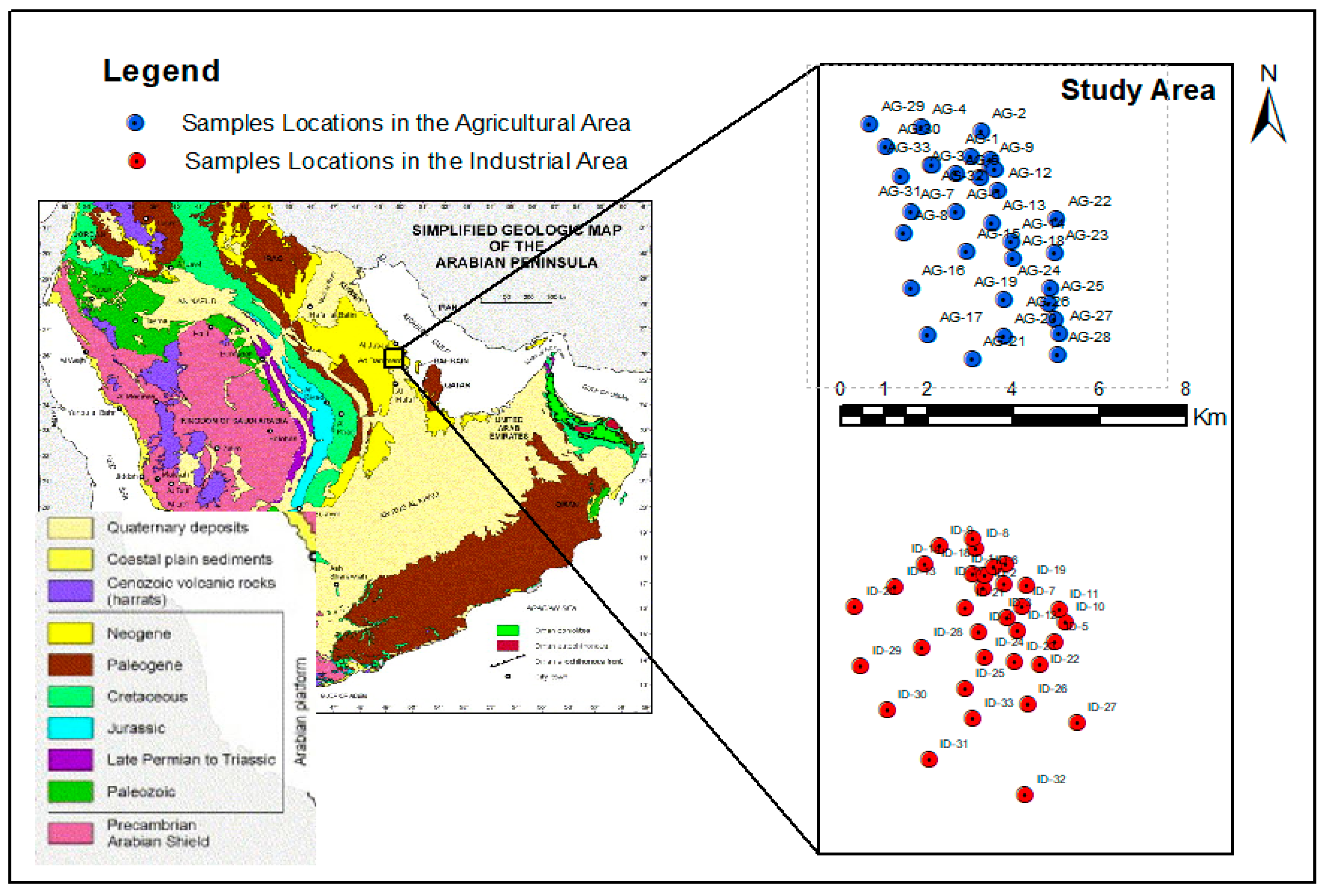
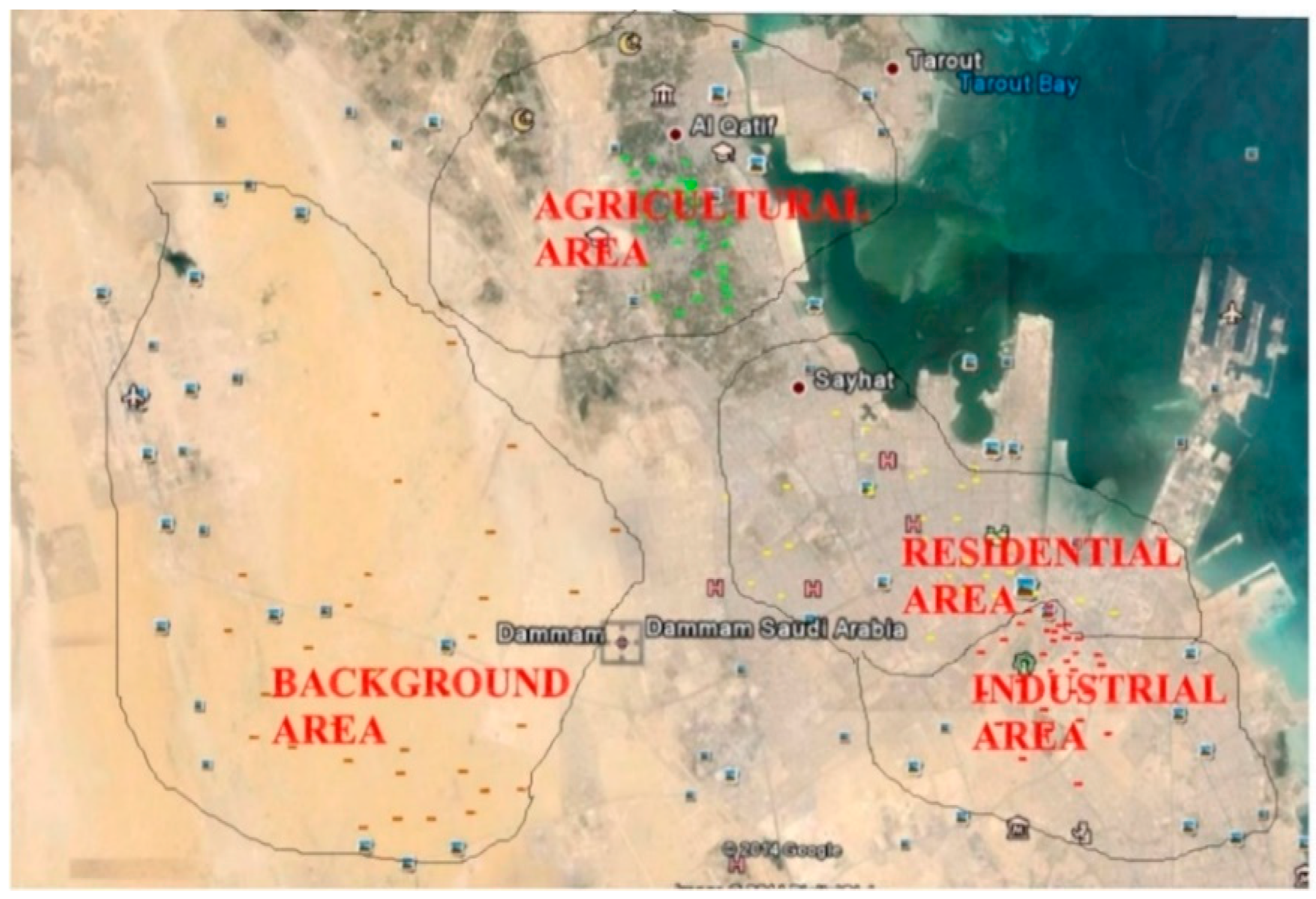
2. Study Area and Sample Locations

Dammam is located between latitudes 26°20′ and 26°32′ and longitudes 49°49′ and 50°09′. It is an important port on the Arabian Gulf in the east of Saudi Arabia. It is the largest city in the eastern region with a population of over a million. The most important centers in the world for the production and refining of petroleum are located close by. It is also surrounded by many farms that produce dates and other fruits and vegetables. It also has two (2) main industrial cities for small to medium size industries. Dammam has recently experienced migration, sub-urbanization, and rapid industrialization. As stated above, the geological Map and AG and ID areas were considered and are presented in Figure 1. The top soil samples were collected in 132 locations from 4 different locations in the Dammam area over a two (2) month period (i.e., February to March 2014). The procedure is considered as a powerful acid digesting process capable of dissolving all elements that are naturally widespread in the environment.

3. Proposed Methodology

The modelling was carried out using the experimental data on the trace metals levels in the topsoil of the Dammam Area, Saudi Arabia. The average and standard deviation of each factor under consideration for each zone are included in the data summary. Each trace metal’s concentration is measured in milligrams per kilogram of body weight. Data (inputs and outputs) were prepared for each of the eleven (11) elements under study, namely Arsenic (As), Barium (Ba), Cadmium (Cd), Chromium (Cr), Copper (Cu), Mercury (Hg), Nickel (Ni), Lead (Pb), Titanium (Ti), Vanadium (V), and Zinc (Zn). The viability of using soft computing to estimate trace metals was investigated in this work. As a result, selecting the best methodology or the most appropriate solution for a particular situation is challenging for forecasters. Data pre-processing such as data normalization, outlier removal, cleaning, and detecting the missing data was carried out for all the inputs and outputs before the development of the models, and cross-validation was employed to ensure there was no overfitting or underfitting in the training and testing data. The splitting of the data was performed using 70% for calibration and 30% for verification [34,35,36]. Furthermore, 10-k-fold cross-validation was employed during the modelling. In this technique, the data is split into k-fold equal number of sets. On the first trial, the first set was used as the test data, while the remaining sets were used to train the model. On the subsequent trial, the second set was used as the test set. In reality, determining whether one feature selection is superior to another is challenging. Hence this study employed correlation-based feature selection to understand the relationship between the AG and ID stations (Figure 2a,b).

3.1. Analysis of Soil Sampling

Experimental samples were produced according to the USEPA technique 3050B for soil, sediment, and sludge digestion [37]. Subsequently, they were evaluated using an Inductively Coupled Plasma-optical Emission Spectrometer (ICP-OES), from SPECTRO Analytical Instruments Germany [37]. The chemical reagent employed complied with the standards of the ACSCAR (American Chemical Society’s Committee on Analytical Reagents). Distilled water (DI), concentrated nitric acid (HNO3), concentrated hydrochloric acid (HCl), and 30% hydrogen peroxide are examples of such reagents (H2O2). Because the digestion required the use of acid, it was done in a fume hood under the supervision of an expert and with the certified and recommended laboratory safety equipment. The equipment was calibrated using a multi-element standard solution. To confirm the equipment’s appropriateness and accuracy, six working standard samples and one blank were used. Each batch of processed samples was also subjected to quality control techniques. Each batch had 20 samples: one duplicate, two spiked samples, two blank samples, and two standard samples.
For sampling purposes, the Dammam area was divided into four (4) zones: residential (R), industrial (ID), agricultural (AG), and background (BG) areas; however, for this study, only the AG and ID areas were considered, as shown in Figure 3. The background area was selected west of Dammam, away from any known industrial, agriculture, or residential activities. From each zone, 33 representative samples were collected, with a total of 132 samples. Representative soil samples of a uniform soil type in each sampling zone were collected using an auger at a depth of 10–15 cm. Geographical coordinates of all sample locations were recorded with the aid of handheld Global Positioning System (GPS) instruments (Garmen Handheld, ETrex 20). However, google maps, google street view, and satellite imagery were used in deciding the best sample locations and also helped in avoiding sampling repetition. The samples collected were then stored in polythene bags, placed in a hard box casing, and transported to the environmental laboratory at the Geosciences Department of KFUPM.

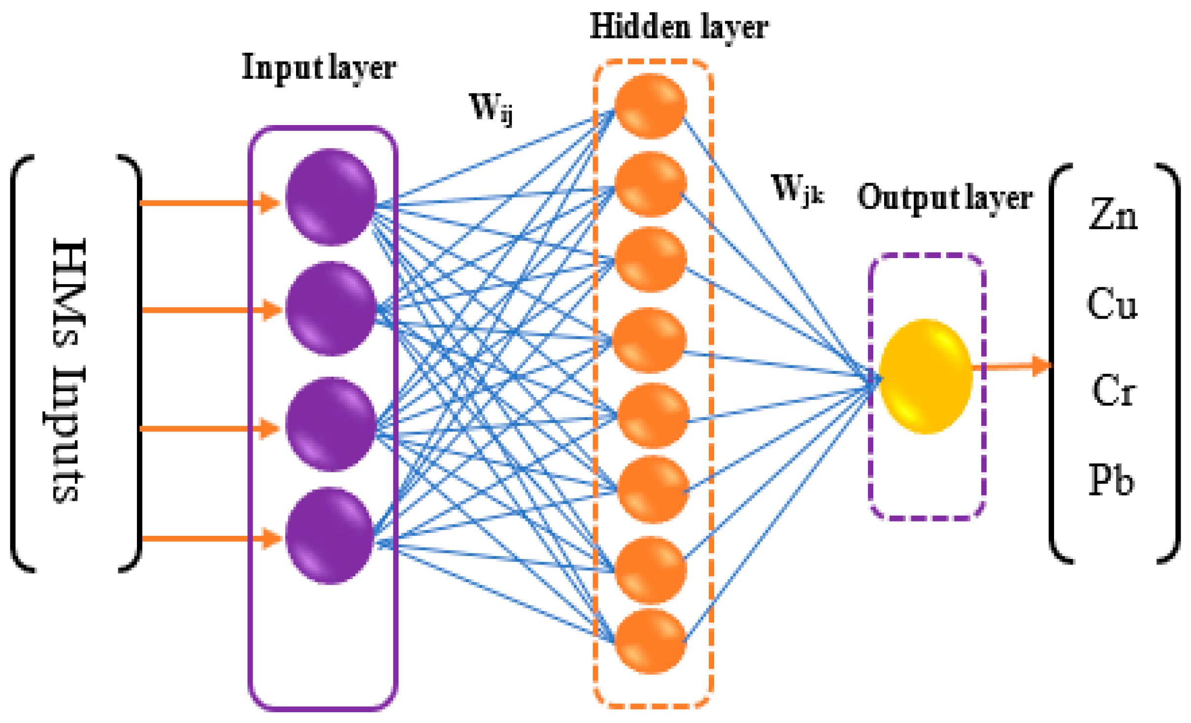
3.2. Artificial Neural Network (ANN)

The ANN is a form of artificial intelligence based on the study of human neurons to simulate how the human brain processes information [38]. It is a computational model that produces outputs of the received inputs through several processing elements based on their predefined activation function. It has the ability to analyze the relationship between the inputs from multiple sources in an intuitive way [39] (Figure 4). For soil application, the ANN has been used to predict soil properties with reasonable accuracy by several researchers. Licznar and Nearing [40] used the ANN to predict soil erosion and runoff. Ramadan et al. [41] applied the ANN to estimate the percentage of some soil properties (clay, sand, silt, and organic carbon) from a microbial community DNA dataset. Zhao et al. [42] produced high-resolution maps of soil properties (soil texture, soil organic carbon, and soil drainage) based on DEM-generated topo-hydrological data.

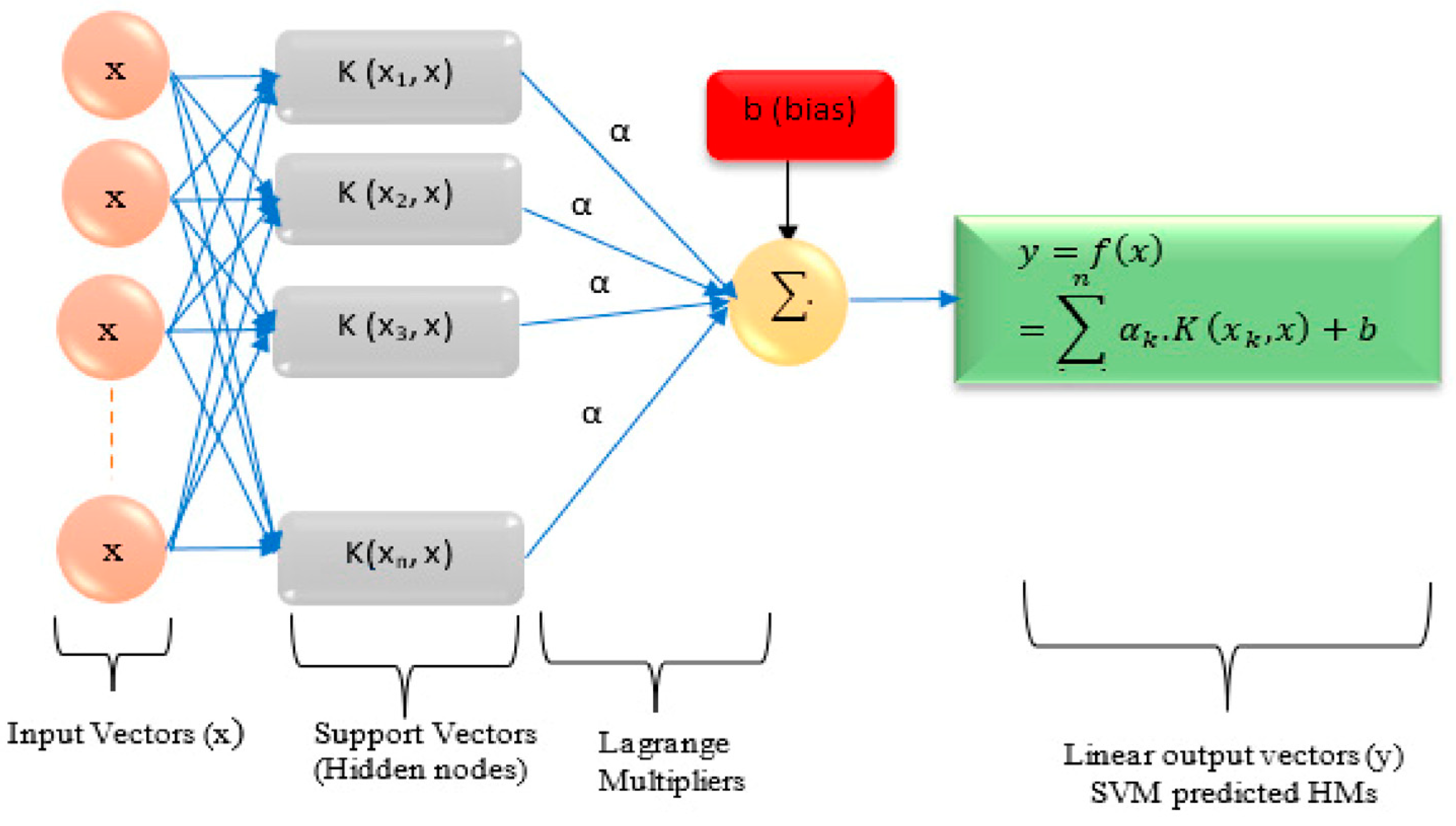
3.3. Support Vector Regression (SVR)

A support vector machine (SVR) is a machine learning technique that is widely used to perform classification and regression analysis using data analysis and pattern recognition [43,44]. It was developed by Vapnik [45], as shown in Figure 5. The SVR has been used as a standalone technique or combined with other machine learning techniques (e.g., ANN) to predict, map, and model soil properties (e.g., soil moisture, infiltration rate, soil salinity, organic content, total hydrocarbon etc.) in several studies, such as [46,47,48,49,50,51]. In the literature, it has been reported that SVR models have been utilized by several researchers to estimate the concentration of trace and heavy metals in soil [52,53,54]. Equation (1) represents the SVR function with notations xk and m as the support vectors and their numbers, while the bias term (b) and the Lagrange coefficient α ¯ k need to be determined analytically for optimal SVR network identification.
f ( x ) = k = 1 m α ¯ k . K ( x k , x ) + b

3.4. ‘Top Soil’s Trace Metal Impact on Subsurface Water Quality

In this regard, the issue of groundwater interaction with polluted soil is equally crucial. This research intends to create spatial concentrations of HMs in the region’s topsoil, the “hot spot” area, and the regional distribution of the pollutants, allowing the authorities to monitor company operations and offer a decent quality of life for the general population. The presence of high quantities of trace metals in soil can contaminate groundwater. These substances can enter aquifers through a variety of mechanisms. HMs with geological formation; underground water contacts with the surface that contain such metals; percolation of precipitation water, including dissolved, colloidal, and suspended materials; and direct access from the land surface via wells are examples of such channels. For instance, HMs include metals such as Arsenic (As), which is a naturally occurring element in the earth’s crust. Volcanic ash, degradation of AS-containing minerals, and ores dissolved in groundwater are some of the naturally occurring exposure mechanisms. Food, water, earth, and air contain them [8,12,54].
The water footprint (WF) indicates the amount of freshwater used by consumers or products in direct or indirect ways [55]. It is an accepted international indicator that reflects the human impact on the quantity and quality of water resources [56]. The water footprint consists of three types: GWF (green water footprint), BWF (blue water footprint), and gray WF (gray water footprint). The green water footprint (GWF) indicates the volume of rainwater consumed to produce a product or service. In other terms, it relates to the quantity of water from rainfall that is either lost by evaporation and transpiration or absorbed by plants after being held in the root zone of the soil (called green water). However, the amount of water obtained from sources such as groundwater and surface bodies are referred to as BWF. This type of water can also originate from several sources, including shallow and deep aquifers, lakes, rivers, and wetlands, which indicates the amount of groundwater and surface water used in the service production [57]. The grey WF refers to the quantity of water used to dilute a certain amount of contamination in order to meet the required standard. Gray WF was introduced to meet the needs of the ambient water quality standards by considering the essential water volume for the dilution of the commercial, agricultural, and mining industries, as well as municipal discharges, ranging from point and non-point sources of pollution. To meet the need of several international health bodies and to maintain environmental sustainability as stated by sustainable development goals, these three WF indicators emerged as essential requirements for measuring environmental indicators (Figure 6).

4. Results and Discussion

The overall well-being of individuals and groups has attracted the global community’s interest for decades. Such well-being cannot be measured purely by income and jobs, but also by the sustainability of the built environment and the inhabitants’ physical and mental health. Dammam has seen significant urbanization and industrialization due to the discovery and production of oil and gas, as well as petrochemical and other industries. The area has become more urbanized due to industrialization, necessitating an evaluation of the topsoil in the area because many of the industries in the vicinity have the potential to release harmful HMs into the ecosystem. As mentioned in Section 1, the complex nature of HMs and associated elements tends to introduce an emerging soft computing knowledge and the internet of things. This study aims to assess different trace elements’ concentrations and spatial distributions at the selected AG and ID zones. Additionally, machine learning is applied for the simulation and modelling of four HMs: Zn, Cu, Cr, and Pb. Other trace elements can also be simulated using the feasibility of the same approach.

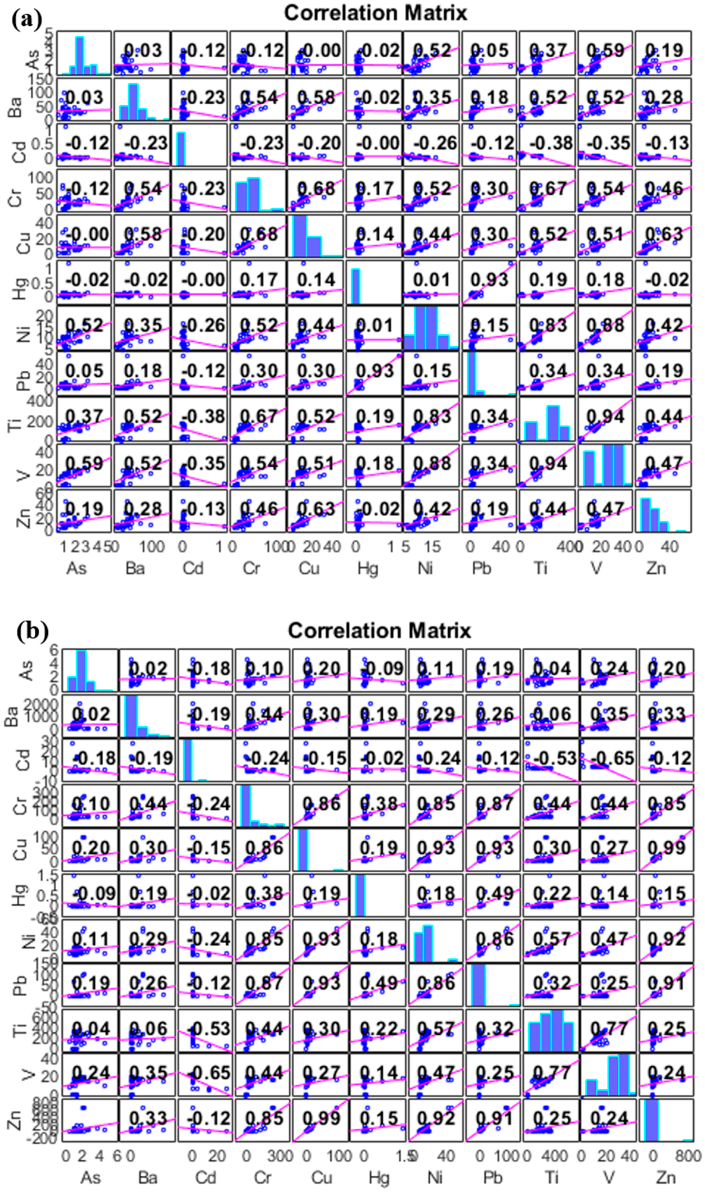
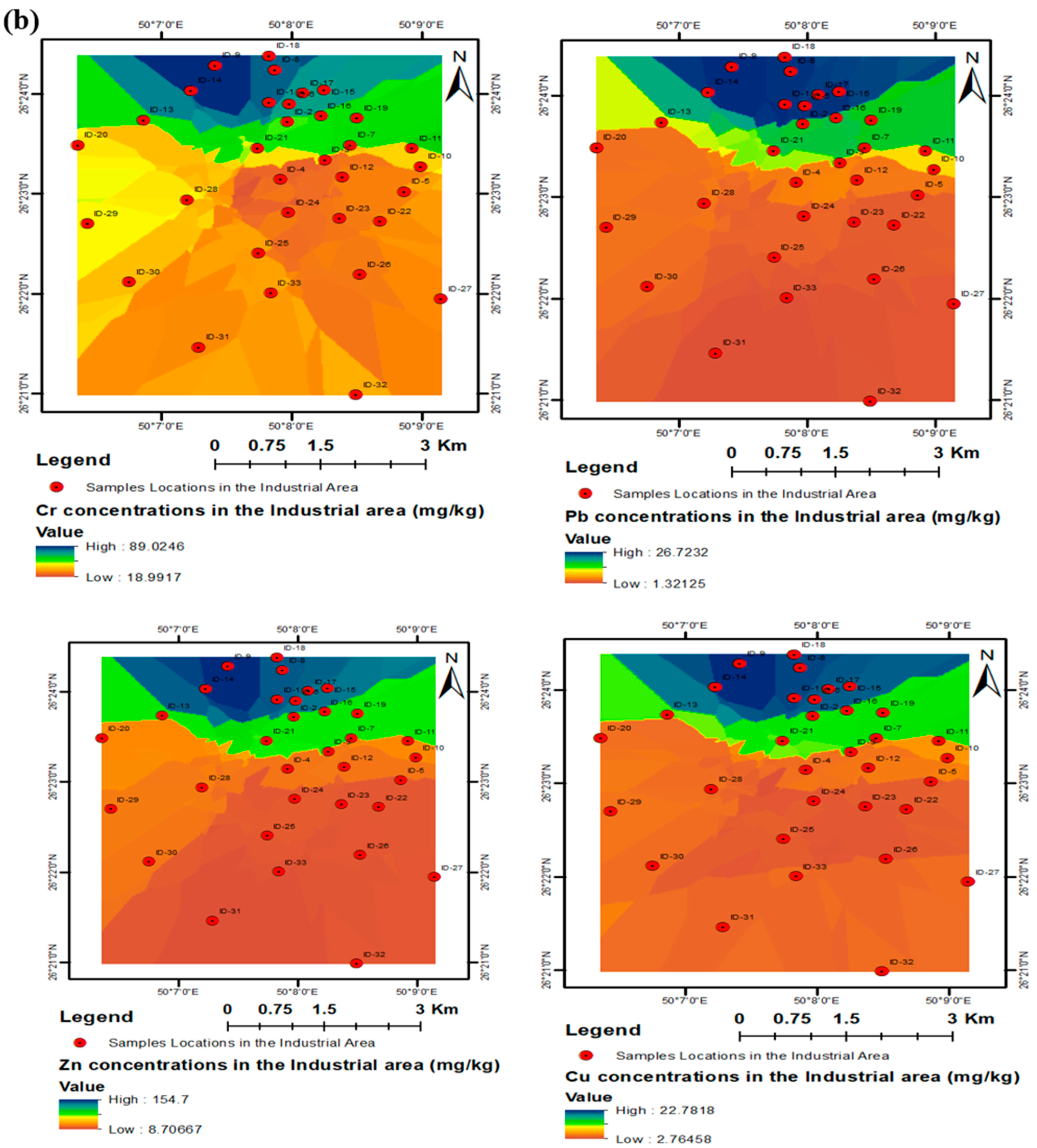
4.1. Spatiotemporal Analysis of Trace Metals

The American Association of State Highway and Transportation Officials (AASHTO) sieve analysis procedure was adopted to assess the concentrations and spatial distributions of different trace elements in the AG and ID areas. This provided a method for addressing soil research through a systematic and thorough methodology. The grain size distribution and soil consistency were used to classify soil characteristics. The topsoil was classified using a unified soil classification method. The geochemical map of the sample sites was created using AutoCAD (Autodesk: San Rafael, CA, USA) and ArcMap (Esri: Redlands, CA, USA) software. During sample collection, a portable GPS was used to record sample locations. The geochemical spatial distribution map of each element discovered in the different regions was then created using Surfer 8 software (Golden Software: Golden, CO, USA). After analysis, the trace metal content in each place was combined with the geographical coordinates of each sample location obtained during sample collection. The levels of metals are presented below in parenthesis with the mean levels followed by the maximum level detected in (mg/kg) in the sampled locations. Since the Kingdom of Saudi Arabia does not have well-defined guidelines regarding the limits of trace metals in soil, the Canadian Environmental Soil Quality Guidelines (CESQG) standards for the Protection of Environment and Human Health (PEHH) were adopted for comparison purposes. The results of the study showed that barium (Ba) was higher in industrial areas (Median = 120.90 mg/kg, Max = 1966.50 mg/kg, Min = 0.00 mg/kg), followed by agricultural (Median = 32.78 mg/kg, Max = 100.650 mg/kg, Min = 7.80 mg/kg), and residential areas (Median = 33.77 mg/kg, Max = 98.55 mg/kg, Min = 0.33 mg/kg) (Figure 7).
Some of the samples from the industrial areas exceeded the allowable limit of 500 mg/kg. The elevated levels of Ba in industrial areas can be associated with the use of Ba compounds or oxides for several industrial activities [58]. Barium nitrate is used in fireworks to give them a green colour. Chromium (Cr) was highest in industrial soil samples (Median = 26.99 mg/kg, Max = 247.60 mg/kg, Min = 0.12 mg/kg), followed by the residential area (Median = 25.65 mg/kg, Max = 120.20 mg/kg, Min = 0.07 mg/kg) and the agricultural areas (Median = 23.12 mg/kg, Max = 74.70 mg/kg, Min = 3.03 mg/kg). Some of the samples from each of the three sampled areas measured above the allowable limit of 74 mg/kg. The elevated levels of Cr in agricultural soil may be attributed either to natural sources or atmospheric deposition of Cr containing compounds, as presented in Figure 7. However, the concentration of Zinc (Zn) was highest in the industrial area (Median = 10.88 mg/kg, Max = 676.50 mg/kg, Min = 0.10 mg/kg), followed by the agricultural (Median = 9.65 mg/kg, Max = 46.73 mg/kg, Min = 1.02 mg/kg) and residential areas (Median = 4.87 mg/kg, Max = 30.54 mg/kg, Min = 0.01 mg/kg). None of the samples exceeded the allowable limit of 200 mg/kg (see, Figure 7). Nickel (Ni) was highest in the industrial area (Median = 11.60 mg/kg, Max = 45.20 mg/kg, Min = 4.76 mg/kg), followed by the agricultural (Median = 8.68 mg/kg, Max = 16.25 mg/kg, Min = 4.60 mg/kg) and residential areas (Median = 6.07 mg/kg, Max = 13.23 mg/kg, Min = 2.25 mg/kg). None of the samples exceeded the allowable limit of 50 mg/kg (see, Figure 7). The Copper (Cu) level was highest in the industrial area (Median = 3.94 mg/kg, Max = 95.75 mg/kg, Min = 0.18 mg/kg), followed by the agricultural (Median = 8.66 mg/kg, Max = 31.64 mg/kg, Min = 0.97 mg/kg) and residential areas (Median = 3.53 mg/kg, Max = 16.80 mg/kg, Min = 0.04 mg/kg). Two of the samples from the industrial area exceeded the allowable limit of 63 mg/kg. The elevated levels of Cu in 2 out of 33 industrial samples may be attributed to the use of Cu in the production of electrical wires, roofing, plumbing, and industrial machinery.
Close analysis also indicated that lead (Pb) was highest in the industrial area (Median = 1.92 mg/kg, Max = 100.25 mg/kg, Min = 0.04 mg/kg), followed by the agricultural (Median = 4.61 mg/kg, Max = 52.35 mg/kg, Min = 0.90 mg/kg) and residential areas (Median = 1.89 mg/kg, Max = 25.60 mg/kg, Min = 0.08 mg/kg). None of the samples exceeded the allowable limit of 140 mg/kg. Lead occurs naturally in the environment in very small amounts. The results also showed that low levels of As, Cd, Hg, and V were detected in the top soil samples collected in the study. As was highest in the industrial area (1.58, 4.56), followed by the agricultural area (1.52, 3.14 mg/kg), while the lowest level was in the residential area (Mean = 0.97 mg/kg, Max = 2.22 mg/kg). However, none of the samples exceeded the threshold of 12 mg/kg. Cadmium (Cd) was highest in the industrial area (Median = 0.05 mg/kg, Max = 28.69 mg/kg, Min = 0.00 mg/kg), followed by the residential area (Median = 0.03 mg/kg, Max = 23.01 mg/kg, Min = 0.00 mg/kg) and the agricultural area (Median = 0.03 mg/kg, Max = 1.14 mg/kg, Min = 0.00 mg/kg). One sample from each of the industrial and agricultural areas measured above the allowable limit of 10 mg/kg. On the other hand, Mercury (Hg) was highest in the industrial area (Median = 0.05 mg/kg, Max = 1.44 mg/kg, Min = 0.01 mg/kg), followed by the agricultural (Median = 0.05 mg/kg, Max = 1.212 mg/kg, Min = 0.00 mg/kg) and residential areas (Median = 0.03 mg/kg, Max = 0.59 mg/kg, Min = 0.00 mg/kg). None of the samples exceeded the allowable limit of 6.6 mg/kg. Vanadium (V) was highest in the industrial area (Median = 14.78 mg/kg, Max = 20.42 mg/kg, Min = 0.09 mg/kg), followed by the agricultural (Median = 12.43 mg/kg, Max = 21.89 mg/kg, Min = 1.64 mg/kg) and residential areas (Median = 7.62 mg/kg, Max = 17.73 mg/kg, Min = 0.02 mg/kg). None of the samples exceeded the allowable limit of 130 mg/kg.

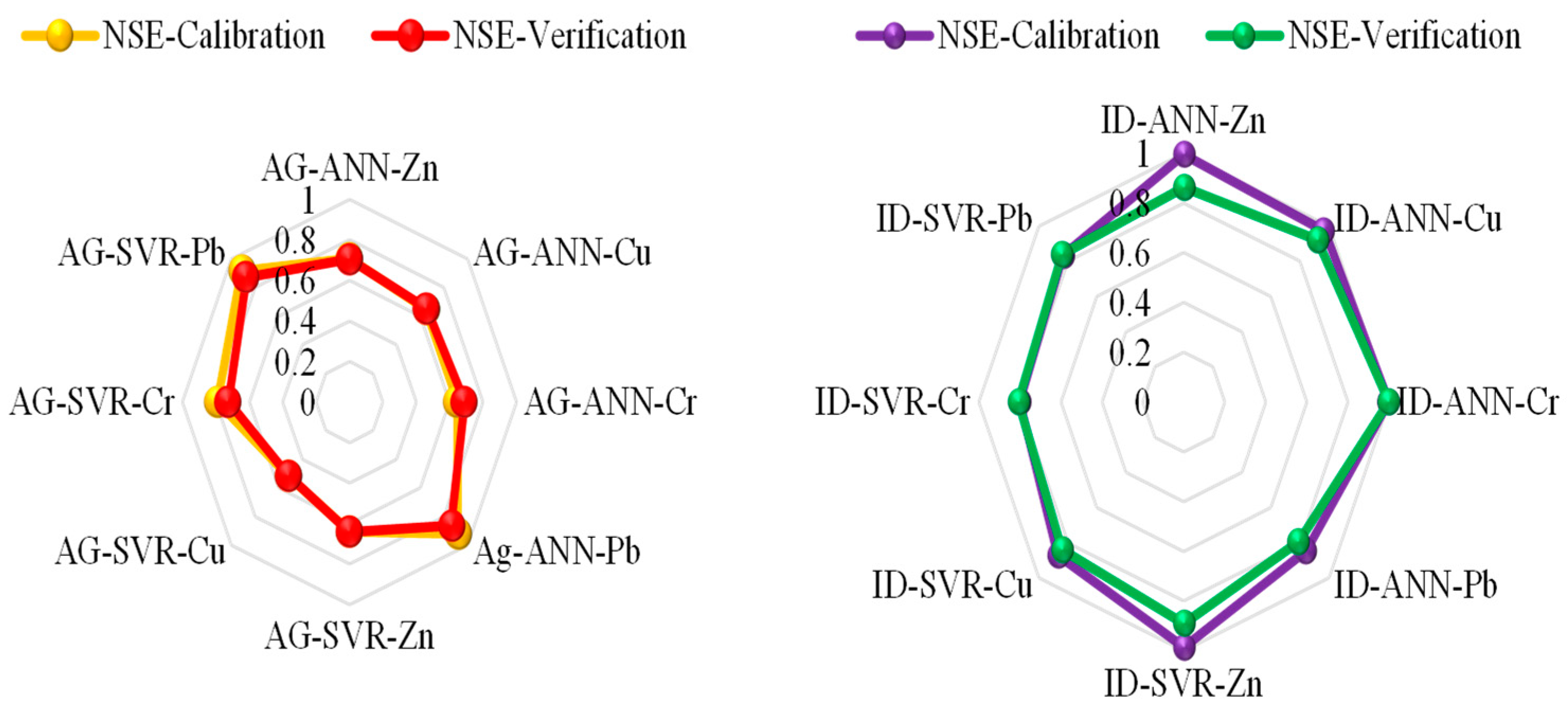
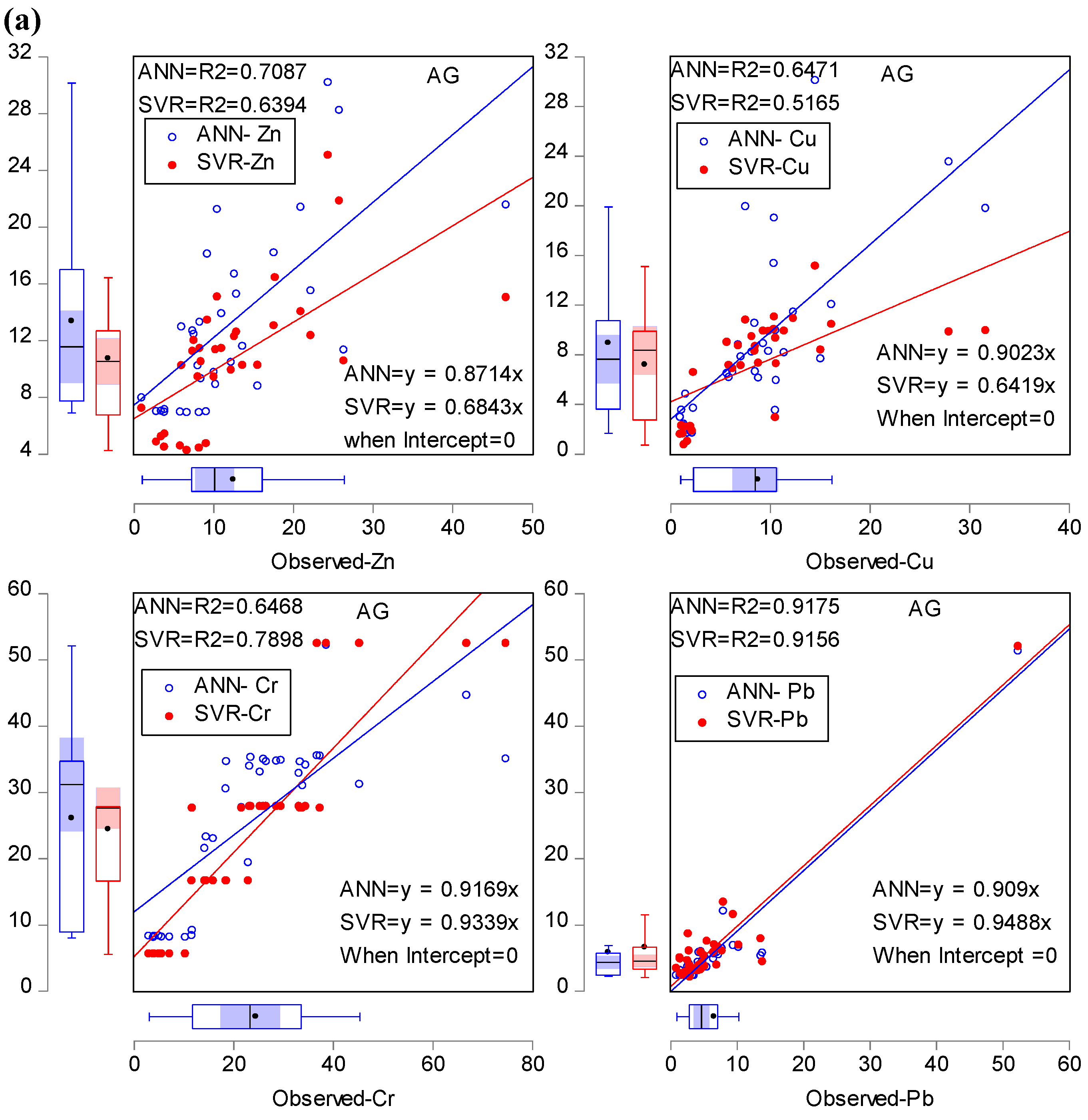
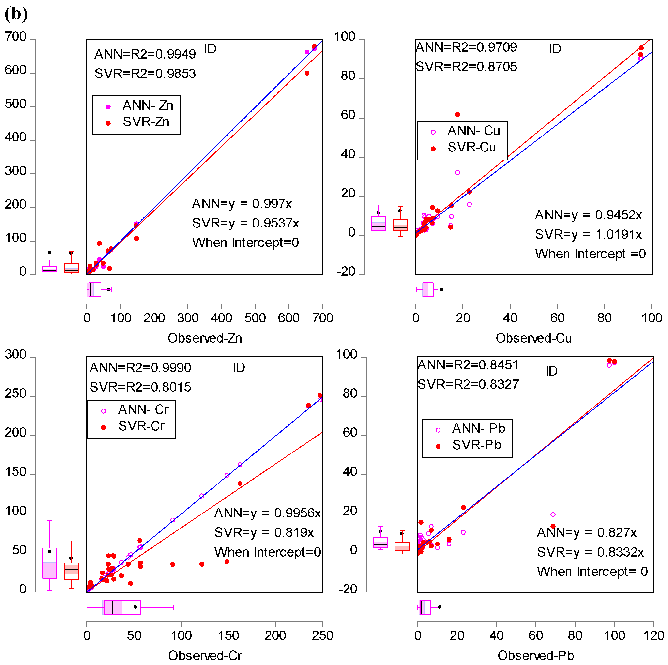
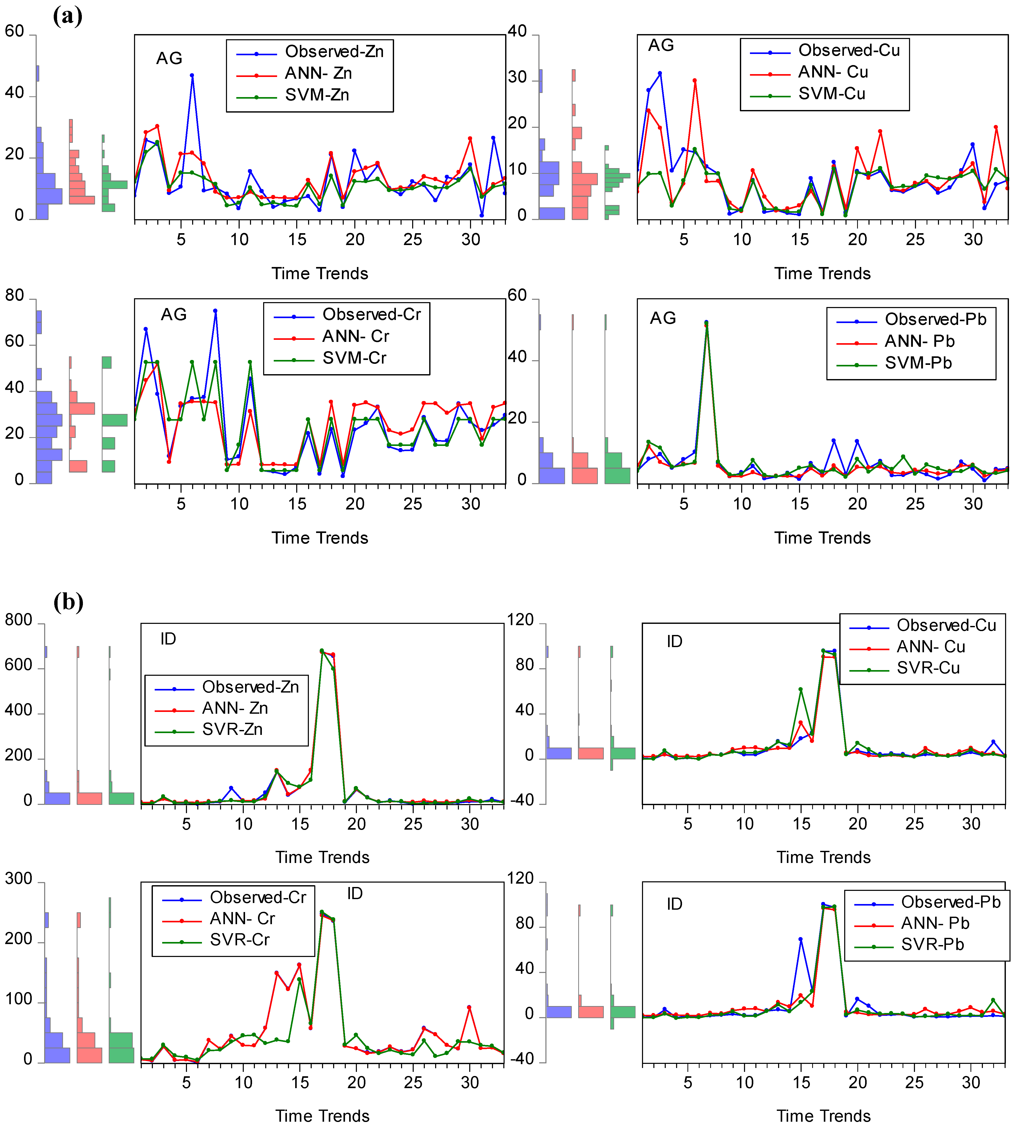
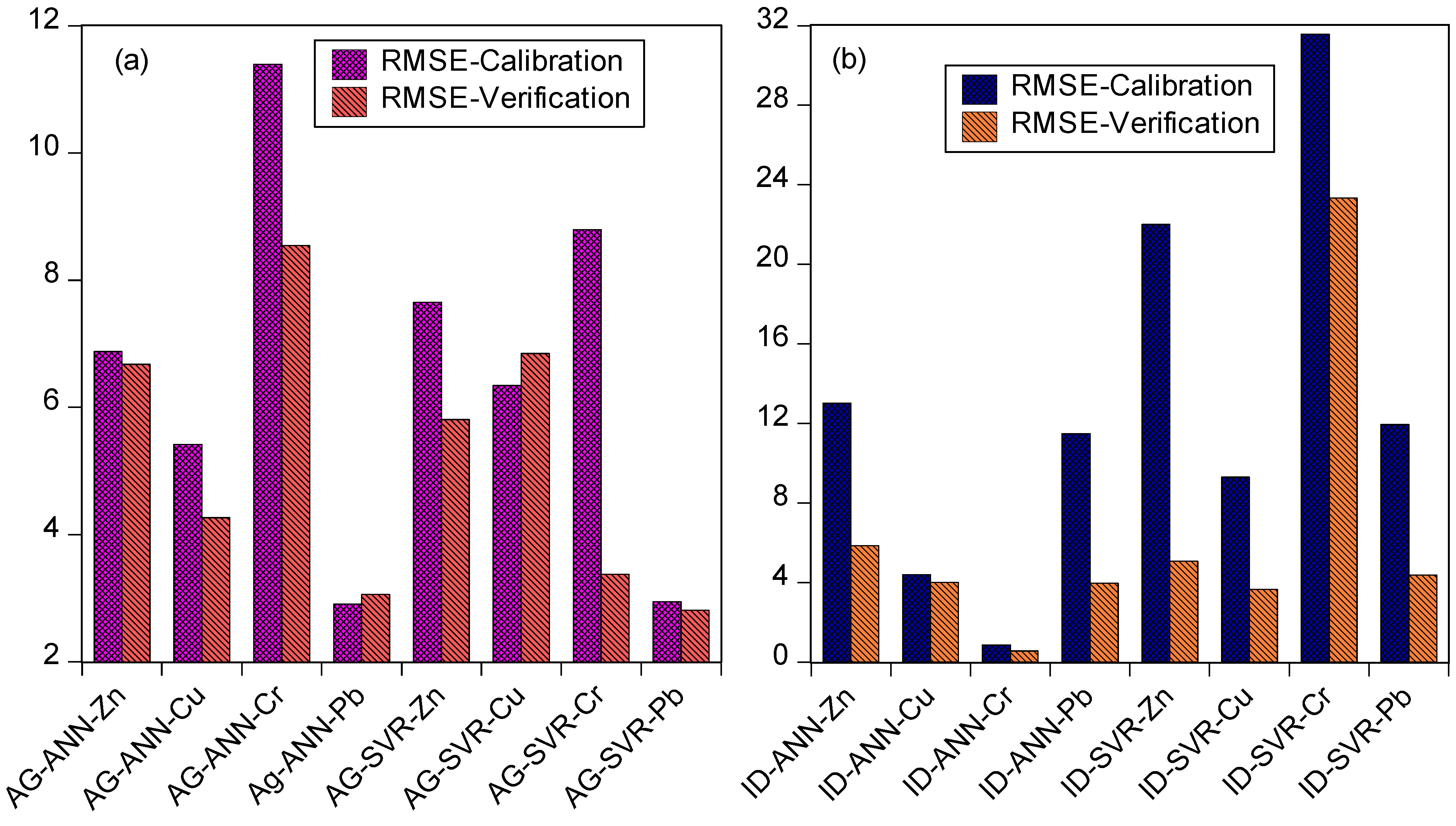
4.2. Simulation Using AI-Based Models

Classical techniques have been adopted for the analytical exploration, extraction, and quantification of trace metals despite several limitations and an unrealistic way of predicting the trace metals. As a result of AI-based technological developments and an industrial 4.0 IoT, a more reliable and understanding estimation of trace metals can now be achieved. To achieve the AI-based objective of this paper, a widely used AI model (ANN) and recently employed machine learning regression (SVM) are explored to simulate four different HMs (Zn, Cu, Cr, and Pb) in the AG and ID regions of Dammam, Saudi Arabia (Figure 8). The sensitive nature of the data and sampling sites has been a focus of global attention recently; on the other hand, AI-based models provide an efficient and economic advantage that leads to strong policies related to trace elements. According to Yaseen [3] it is clear that Zn, Cu, Cr, and Pb are the most explored HMs using soft computing techniques owing to their hazardous nature. The selection of input variable features is crucial for any computational development and can play an influential role in increasing the learning and robustness of the models; this study used a Pearson-based input combination, as mentioned above. For the ANN model, modelling was carried out using several trial-and-error approaches to optimize the best hyper-turning variable, such as hidden nodes, iteration, momentum parameter, and activation constant. Similarly, SVM modelling was fine-tuned to optimize the results. The performance efficacy of the models was evaluated using a statistical variable (NSE, MSE, RMSE). In addition to the effective analysis in terms of the reliability of the predictive models, the quantitative and visual presentations of the findings provide an in-depth understanding of the impact and significance of each parameter of the proximate analysis regarding this determination.
The outcomes of the simulated models are discussed and evaluated in this section for the AG and ID sample stations. The overall results for both the calibration and verification are presented in Table 1. The calibration phase showed that the highest goodness-of-fit for AG and ID are attributed to Zn (ANN = NSE = 0.7087, 0.7038), Cu (ANN = 0.6471, 0.6535), Cr (SVR = 0.7898, 0.7244), Pb (0.9175, 0.8615), Zn (ANN = 0.9947, 0.8624), Cu (0.9709, 0.9203), Cr (0.9999, 0.9994), and Pb (0.8451, 0.7935), respectively. The simulated model performed consistently throughout the calibration and verification modelling processes, as evidenced by the evaluation values of the performance indicators reported. This is common, since the prediction models react differently depending on the simulated dataset’s learning process.
Moreover, this emphasizes that various statistical performance indicators and visualizations are used for the prediction models to be analyzed and evaluated. Further understanding of the results is presented in the form of spider plots in Figure 9. The figure identifies several variations of the NSE value that directly indicate the determination coefficient; the NSE establishes the relative degree of the noise or residual variance compared to the experimental data variance. The NSE values range between AG (51–91% and 51–87%) and ID (80–99% and 79–99%) for calibration and verification, respectively. Based on the reported graphical visualization of spider plots, it can be seen that AI-based models (ANN and SVR) are promising techniques for capturing nonlinear patterns of HMs. Almost all the ID station modelling justified merit with an NSE value above 80%. Some of the results for AG station are within the marginal borderline, which indicates a lot of warning signals with regard to the agricultural station.
For a better examination of the computational result, a graphical visualization was performed using scatter and time series plots. The two graphs can be used to evaluate the produced model’s precision. According to the NSE, the scatter plots of the models in the ANN and SVR models are displayed in Figure 10 (a) AG (b) ID. For most of the models in Figure 10, the accumulation of data points is high, around the 45° line in the scatter plots. The scatter plot has the critical manner of evaluating the performance of the ML model to demonstrate the degree of deviation from the ideal line. Furthermore, as seen in the time series plots, the trend of the predicted HMs closely matches the pattern of the individual experimental HMs (Figure 10). These are arguments for the remarkable correlations between the projected HMs using these models and the experimental HMs, particularly at the ID station. As a result, the models are accurate and consistent in their predictions. To validate the promising capability of ANN and SVR models, Keshavarzi et al. [59] used an ANN to estimate soil phosphorus by combining satellite-based topography and vegetation data with field-based soil data. The ANN has been used to estimate the soil water retention curve based on field-based soil data [60]. Recently, Pham et al. [61] used the ANN to predict the soil coefficient of consolidation as a mechanical parameter to define the compaction or consolidation status of the soil. Khan et al. [62] establish an ANN-predictive model of soil temperature as geotechnical properties of clay-rich soil using a field dataset. Most of these studies have used an ANN to predict the temporal variation of the heavy and trace metals in soil [63]. The SVR is widely used owing to its optimization objective, since it aims to minimize the generalized error bound instead of the sum squared errors between the actual and predicted outputs that are peculiar in polynomial regression. Figure 11 depicts the time series plot for the models.
It is clear that the AI-based model implementation outperformed the traditional models in capturing the pattern of the system. Additionally, careful examination of the error plot in Figure 12 indicates that the ANN model generated the smallest error term of RMSE at both the AG and ID stations. The discrepancies between the range of observed and predicted values in most of the models are within the acceptable limit despite some variations observed for ID-SVR-Cr in the verification phase. The error evaluation criteria depict the extent of the closeness of the predicted results to the observed values. Essentially, lower values are indications of a better correlation of the developed model. It is important to note that various factors influence the concentration of trace elements, including not only physiochemical but also hydrological, climatic, and Lithological factors. As a result, examining the AI model’s capabilities with restricted input data is more advantageous for low-income and developing nations that lack the resources to create a broader range of input variables, such as hydrological and meteorological variables.
To make the fair judgment deep into the current literature, the outcomes are in line with those of Pyo et al. [8], who employed an ANN, a convolutional neural network (CNN), and random forest regression (RFR) for estimating heavy metals in soil (Pb, Cu, AS). It was observed in the study that the R2 value ranged from 0.6–0.94 for both Pb and Cu. In addition, Bazoobandi et al. [7] applied an ANN, ANFIS, and MLR model, and the outcomes showed that the range of R2 was 0.6–0.89 and 0.3–0.93 for ANN and ANFIS, respectively. Because HMs are widely used in agriculture, industry, and other areas, they have become part of the environment, increasing the risk of the metals having a harmful influence on the ecosystem. By enacting legislation to that effect, the United States, for example, has outlawed the use of items suspected of elevating trace metals levels in the soil. For example, the United States Environmental Protection Agency (USEPA) has established specified HM thresholds that must be present in bio-solids before authorization for land spreading can be given. HMS contamination has undeniable consequences for our environment and human health. Although there have been several types of research on pollution in Saudi Arabia, such research has evaluated metals content in marine, coastal, and air environments, with limited research on topsoil.

5. Conclusions

The primary objective of this study was to use an integrated scenario, (i) integrating the GIS to evolve the spatial distribution of HMs in the eastern province of Dammam area, which was accomplished successfully. The outcomes of the field and laboratory tests revealed that some collected samples had exceeded the standard range, and (ii) the study employed AI-based models, namely ANN and SVR, to control and understand the feasibility of simulating trace metals in the topsoil. The concentration of ten essential trace metals in the soils of the Dammam area followed a general trend in almost all metals. They were found at higher concentrations in the samples taken from the soils of industrial areas, followed by agricultural and residential areas. Only in a few of the samples were the maximum levels higher than the allowable limits. However, the mean concentration of all metals exceeded the allowable thresholds. These findings provide relief that the concentrations of all the metals studied were within acceptable limits, and they pose no immediate threat to the environment. Ultimately, the natural environmental resources, as well as animal and human health, might be exposed to the risks/hazards associated with these metals. The modelling approach indicated that ANN and SVR models are capable of estimating the HMs with high accuracy, especially in the ID stations. However, AG stations are within the range of marginal-to-good accuracy. This showed that more robust models need to be explored, such as adaptive neuro-fuzzy inference systems (ANFIS), Elman neural networks, extreme learning machines (ELM), hybrid models, and optimization algorithms, to boost the accuracy of the predictions.

Author Contributions

Conceptualization, B.T. and S.I.A.; methodology, S.I.A., M.B., M.A.Y. and J.A.A.; validation, M.A.Y., M.B. and S.I.A.; formal analysis. B.T., S.I.A. and J.A.A.; investigation, S.I.A., M.A.Y., J.A.A. and M.B.; resources, S.I.A., J.A.A. and M.A.Y.; data curation, J.A.A. and A.A.-S.; writing—original draft preparation, B.T., S.I.A., M.A.Y., M.B., J.A.A. and A.A.-S.; writing—review and editing, S.I.A.; visualization, M.A.Y. and S.I.A.; supervision, M.A.Y. and B.T.; project administration, B.T. and A.A.-S.; funding acquisition, A.A.-S. and B.T. All authors have read and agreed to the published version of the manuscript.

Funding

This research was funded by King Fahd University of Petroleum and Minerals.

Institutional Review Board Statement

Not applicable.

Informed Consent Statement

Not applicable.

Data Availability Statement

Available based on request.

Acknowledgments

Authors would like to acknowledge all support provided by the Interdisciplinary Research Center for Membrane and Water Security, King Fahd University of Petroleum and Minerals. The authors also would like to acknowledge College of Petroleum Engineering and Geosciences, King Fahd University of Petroleum and Minerals for all support and assistance provided for fieldwork and laboratory analysis.

Conflicts of Interest

The authors declare no conflict of interest.

References

  1. Kiiza, C.; Pan, S.-Q.; Bockelmann-Evans, B.; Babatunde, A. Predicting pollutant removal in constructed wetlands using artificial neural networks (ANNs). Water Sci. Eng. 2020, 13, 14–23. [Google Scholar] [CrossRef]
  2. Therrien, J.-D.; Nicolaï, N.; Vanrolleghem, P.A. A critical review of the data pipeline: How wastewater system operation flows from data to intelligence. Water Sci. Technol. 2020, 82, 2613–2634. [Google Scholar] [CrossRef] [PubMed]
  3. Yaseen, Z.M. An insight into machine learning models era in simulating soil, water bodies and adsorption heavy metals: Review, challenges and solutions. Chemosphere 2021, 277, 130126. [Google Scholar] [CrossRef] [PubMed]
  4. Wang, H.; Yilihamu, Q.; Yuan, M.; Bai, H.; Xu, H.; Wu, J. Prediction models of soil heavy metal(loid)s concentration for agricultural land in Dongli: A comparison of regression and random forest. Ecol. Indic. 2020, 119, 106801. [Google Scholar] [CrossRef]
  5. Wang, X.; Li, X.; Ma, R.; Li, Y.; Wang, W.; Huang, H.; Xu, C.; An, Y. Quadratic discriminant analysis model for assessing the risk of cadmium pollution for paddy fields in a county in China. Environ. Pollut. 2018, 236, 366–372. [Google Scholar] [CrossRef]
  6. Zhang, X.; Lin, F.; Jiang, Y.; Wang, K.; Wong, M.T. Assessing soil Cu content and anthropogenic influences using decision tree analysis. Environ. Pollut. 2008, 156, 1260–1267. [Google Scholar] [CrossRef]
  7. Allen, A.; Nemitz, E.; Shi, J.; Harrison, R.; Greenwood, J. Size distributions of trace metals in atmospheric aerosols in the United Kingdom. Atmos. Environ. 2001, 35, 4581–4591. [Google Scholar] [CrossRef]
  8. Alloway, B.J. Trace Metals and Metalloids in Soils and their Bioavailability; Springer: Cham, Switzerland, 2018. [Google Scholar]
  9. Abadin, H.; Ashizawa, A.; Stevens, Y.-W.; Llados, F.; Diamond, G.; Sage, G.; Citra, M.; Quinones, A.; Bosch, S.J.; Swarts, S.G. Toxicological Profile for Lead; Agency for Toxic Substances and Disease Registry: Atlanta, GA, USA, 2007; p. 582.
  10. Ramelli, G.; Taddeo, I.; Herrmann, U.; Weber, P. V13 Poster location 013 Paroxysmal tonic upgaze of infancy: 5 additional cases. Eur. J. Paediatr. Neurol. 2009, 13, S10. [Google Scholar] [CrossRef]
  11. Bazoobandi, A.; Emamgholizadeh, S.; Ghorbani, H. Estimating the amount of cadmium and lead in the polluted soil using artificial intelligence models. Eur. J. Environ. Civ. Eng. 2019, 1–19. [Google Scholar] [CrossRef]
  12. Pyo, J.; Hong, S.M.; Kwon, Y.S.; Kim, M.S.; Cho, K.H. Estimation of heavy metals using deep neural network with visible and infrared spectroscopy of soil. Sci. Total Environ. 2020, 741, 140162. [Google Scholar] [CrossRef]
  13. Yu, K.; Ren, J.; Zhao, Y. Principles, developments and applications of laser-induced breakdown spectroscopy in agriculture: A review. Artif. Intell. Agric. 2020, 4, 127–139. [Google Scholar] [CrossRef]
  14. Wei, L.; Yuan, Z.; Yu, M.; Huang, C.; Cao, L. Estimation of Arsenic Content in Soil Based on Laboratory and Field Reflectance Spectroscopy. Sensors 2019, 19, 3904. [Google Scholar] [CrossRef] [PubMed] [Green Version]
  15. Shi, T.; Chen, Y.; Liu, Y.; Wu, G. Visible and near-infrared reflectance spectroscopy—An alternative for monitoring soil contamination by heavy metals. J. Hazard. Mater. 2014, 265, 166–176. [Google Scholar] [CrossRef] [PubMed]
  16. Sihag, P.; Keshavarzi, A.; Kumar, V. Comparison of different approaches for modeling of heavy metal estimations. SN Appl. Sci. 2019, 1, 780. [Google Scholar] [CrossRef] [Green Version]
  17. Alamrouni, A.; Aslanova, F.; Mati, S.; Maccido, H.S.; Jibril, A.A.; Usman, A.G.; Abba, S.I. Multi-Regional Modeling of Cumulative COVID-19 Cases Integrated with Environmental Forest Knowledge Estimation: A Deep Learning Ensemble Approach. Int. J. Environ. Res. Public Health 2022, 19, 738. [Google Scholar] [CrossRef] [PubMed]
  18. Hadi, S.J.; Abba, S.I.; Sammen, S.S.; Salih, S.Q.; Al-Ansari, N.; Yaseen, Z.M. Non-Linear Input Variable Selection Approach Integrated with Non-Tuned Data Intelligence Model for Streamflow Pattern Simulation. IEEE Access 2019, 7, 141533–141548. [Google Scholar] [CrossRef]
  19. Tiyasha; Tung, T.M.; Yaseen, Z.M. A survey on river water quality modelling using artificial intelligence models: 2000–2020. J. Hydrol. 2020, 585, 124670. [Google Scholar] [CrossRef]
  20. Tao, H.; Salih, S.; Oudah, A.Y.; Abba, S.I.; Ameen, A.M.S.; Awadh, S.M.; Alawi, O.A.; Mostafa, R.R.; Surendran, U.P.; Yaseen, Z.M. Development of new computational machine learning models for longitudinal dispersion coefficient determination: Case study of natural streams, United States. Environ. Sci. Pollut. Res. 2022, 1–21. [Google Scholar] [CrossRef]
  21. Malami, S.I.; Anwar, F.H.; Abdulrahman, S.; Haruna, S.; Ali, S.I.A.; Abba, S. Implementation of hybrid neuro-fuzzy and self-turning predictive model for the prediction of concrete carbonation depth: A soft computing technique. Results Eng. 2021, 10, 100228. [Google Scholar] [CrossRef]
  22. Elkiran, G.; Nourani, V.; Abba, S.I. Multi-step ahead modelling of river water quality parameters using ensemble artificial intelligence-based approach. J. Hydrol. 2019, 577, 123962. [Google Scholar] [CrossRef]
  23. Malami, S.I.; Musa, A.A.; Haruna, S.I.; Aliyu, U.U.; Usman, A.G.; Abdurrahman, M.I.; Bashir, A.; Abba, S.I. Implementation of soft-computing models for prediction of flexural strength of pervious concrete hybridized with rice husk ash and calcium carbide waste. Model. Earth Syst. Environ. 2021, 1–15. [Google Scholar] [CrossRef]
  24. Haruna, S.I.; Malami, S.I.; Adamu, M.; Usman, A.G.; Farouk, A.; Ali, S.I.A.; Abba, S.I. Compressive Strength of Self-Compacting Concrete Modified with Rice Husk Ash and Calcium Carbide Waste Modeling: A Feasibility of Emerging Emotional Intelligent Model (EANN) Versus Traditional FFNN. Arab. J. Sci. Eng. 2021, 46, 11207–11222. [Google Scholar] [CrossRef]
  25. Musa, B.; Yimen, N.; Abba, S.; Adun, H.; Dagbasi, M. Multi-State Load Demand Forecasting Using Hybridized Support Vector Regression Integrated with Optimal Design of Off-Grid Energy Systems—A Metaheuristic Approach. Processes 2021, 9, 1166. [Google Scholar] [CrossRef]
  26. Mahmoud, K.; Bebiş, H.; Usman, A.G.; Salihu, A.N.; Gaya, M.S.; Dalhat, U.F.; Abdulkadir, R.A.; Jibril, M.B.; Abba, S.I. Prediction of the effects of environmental factors towards COVID-19 outbreak using AI-based models. IAES Int. J. Artif. Intell. (IJ-AI) 2021, 10, 35–42. [Google Scholar] [CrossRef]
  27. Yaseen, Z.M.; Sulaiman, S.O.; Deo, R.C.; Chau, K.-W. An enhanced extreme learning machine model for river flow forecasting: State-of-the-art, practical applications in water resource engineering area and future research direction. J. Hydrol. 2018, 569, 387–408. [Google Scholar] [CrossRef]
  28. Abba, S.I.; Abdulkadir, R.A.; Sammen, S.S.; Usman, A.G.; Meshram, S.G.; Malik, A.; Shahid, S. Comparative implementation between neuro-emotional genetic algorithm and novel ensemble computing techniques for modelling dissolved oxygen concentration. Hydrol. Sci. J. 2021, 66, 1584–1596. [Google Scholar] [CrossRef]
  29. Sammen, S.S.; Ehteram, M.; Abba, S.I.; Abdulkadir, R.A.; Ahmed, A.N.; El-Shafie, A. A new soft computing model for daily streamflow forecasting. Stoch. Hydrol. Hydraul. 2021, 35, 2479–2491. [Google Scholar] [CrossRef]
  30. Pham, Q.B.; Abba, S.I.; Usman, A.G.; Linh, N.T.T.; Gupta, V.; Malik, A.; Costache, R.; Vo, N.D.; Tri, D.Q. Potential of Hybrid Data-Intelligence Algorithms for Multi-Station Modelling of Rainfall. Water Resour. Manag. 2019, 33, 5067–5087. [Google Scholar] [CrossRef]
  31. Pham, Q.B.; Gaya, M.; Abba, S.; Abdulkadir, R.; Esmaili, P.; Linh, N.T.T.; Sharma, C.; Malik, A.; Khoi, D.N.; Dung, T.D.; et al. Modelling of Bunus regional sewage treatment plant using machine learning approaches. Desalination Water Treat. 2020, 203, 80–90. [Google Scholar] [CrossRef]
  32. Lakshmi, D.; Akhil, D.; Kartik, A.; Gopinath, K.P.; Arun, J.; Bhatnagar, A.; Rinklebe, J.; Kim, W.; Muthusamy, G. Artificial intelligence (AI) applications in adsorption of heavy metals using modified biochar. Sci. Total Environ. 2021, 801, 149623. [Google Scholar] [CrossRef]
  33. Kazemi, S.; Hosseini, S. Comparison of spatial interpolation methods for estimating heavy metals in sediments of Caspian Sea. Expert Syst. Appl. 2011, 38, 1632–1649. [Google Scholar] [CrossRef]
  34. Usman A., G.; Işik, S.; Abba, S.I. A Novel Multi-model Data-Driven Ensemble Technique for the Prediction of Retention Factor in HPLC Method Development. Chromatographia 2020, 83, 933–945. [Google Scholar] [CrossRef]
  35. Usman, A.G.; Işik, S.; Abba, S.I.; Meriçli, F. Chemometrics-based models hyphenated with ensemble machine learning for retention time simulation of isoquercitrin in Coriander sativum L. using high-performance liquid chromatography. J. Sep. Sci. 2020, 44, 843–849. [Google Scholar] [CrossRef] [PubMed]
  36. Abba, S.I.; Pham, Q.B.; Usman, A.G.; Linh, N.T.T.; Aliyu, D.S.; Nguyen, Q.; Bach, Q.-V. Emerging evolutionary algorithm integrated with kernel principal component analysis for modeling the performance of a water treatment plant. J. Water Process. Eng. 2020, 33, 101081. [Google Scholar] [CrossRef]
  37. Yeskis, D.; Zavala, B. Ground-Water Sampling Guidelines for Superfund and RCRA Project Managers; U.S. Environmental Protection Agency: Chicago, IL, USA, 2022.
  38. Alas, M.; Ali, S.I.A.; Abdulhadi, Y.; Abba, S.I. Experimental Evaluation and Modeling of Polymer Nanocomposite Modified Asphalt Binder Using ANN and ANFIS. J. Mater. Civ. Eng. 2020, 32, 04020305. [Google Scholar] [CrossRef]
  39. Eshragh, F.; Pooyandeh, M.; Marceau, D.J. Automated negotiation in environmental resource management: Review and assessment. J. Environ. Manag. 2015, 162, 148–157. [Google Scholar] [CrossRef]
  40. Licznar, P.; Nearing, M.A. Artificial neural networks of soil erosion and runoff prediction at the plot scale. Catena 2003, 51, 89–114. [Google Scholar] [CrossRef]
  41. Ramadan, Z.; Hopke, P.K.; Johnson, M.J.; Scow, K.M. Application of PLS and back-propagation neural networks for the es-timation of soil properties. Chemom. Intell. Lab. Syst. 2005, 75, 23–30. [Google Scholar] [CrossRef]
  42. Zhao, Z.; Meng, F.-R.; Yang, Q.; Zhu, H. Using Artificial Neural Networks to Produce High-Resolution Soil Property Maps. In Advanced Applications for Artificial Neural Networks; El-Shahat, A., Ed.; IntechOpen: London, UK, 2017. [Google Scholar] [CrossRef] [Green Version]
  43. Guzman, S.M.; Paz, J.O.; Tagert, M.L.M.; Mercer, A.E. Evaluation of Seasonally Classified Inputs for the Prediction of Daily Groundwater Levels: NARX Networks Vs Support Vector Machines. Environ. Model. Assess. 2018, 24, 223–234. [Google Scholar] [CrossRef]
  44. Karmy, J.P.; López, J.; Maldonado, S. Simultaneous model construction and noise reduction for hierarchical time series via Support Vector Regression. Knowl.-Based Syst. 2021, 232, 107492. [Google Scholar] [CrossRef]
  45. Vapnik, V.N. The Nature of Statistical Learning Theory; Springer: Cham, Switzerland, 1995. [Google Scholar]
  46. Akinpelu, A.A.; Ali, E.; Owolabi, T.O.; Johan, M.R.; Saidur, R.; Olatunji, S.O.; Chowdbury, Z. A support vector regression model for the prediction of total polyaromatic hydrocarbons in soil: An artificial intelligent system for mapping environmental pollution. Neural Comput. Appl. 2020, 32, 14899–14908. [Google Scholar] [CrossRef]
  47. Achieng K., O. Modelling of soil moisture retention curve using machine learning techniques: Artificial and deep neural net-works vs. support vector regression models. Comput. Geosci. 2019, 133, 104320. [Google Scholar] [CrossRef]
  48. Taghizadeh-Mehrjardi, R.; Schmidt, K.; Toomanian, N.; Heung, B.; Behrens, T.; Mosavi, A.; Band, S.S.; Amirian-Chakan, A.; Fathabadi, A.; Scholten, T. Improving the spatial prediction of soil salinity in arid regions using wavelet transformation and support vector regression models. Geoderma 2020, 383, 114793. [Google Scholar] [CrossRef]
  49. Were, K.; Bui, D.T.; Dick, Ø.B.; Singh, B.R. A comparative assessment of support vector regression, artificial neural networks, and random forests for predicting and mapping soil organic carbon stocks across an Afromontane landscape. Ecol. Indic. 2015, 52, 394–403. [Google Scholar] [CrossRef]
  50. Sihag, P.; Tiwari, N.K.; Ranjan, S. Support vector regression-based modeling of cumulative infiltration of sandy soil. ISH J. Hydraul. Eng. 2018, 26, 44–50. [Google Scholar] [CrossRef]
  51. Pasolli, L.; Notarnicola, C.; Bruzzone, L. Estimating Soil Moisture with the Support Vector Regression Technique. IEEE Geosci. Remote Sens. Lett. 2011, 8, 1080–1084. [Google Scholar] [CrossRef]
  52. Liu, N.; Zhao, G.; Liu, G. Accurate SWASV detection of Cd (II) under the interference of Pb (II) by coupling support vector re-gression and feature stripping currents. J. Electroanal. Chem. 2021, 889, 115227. [Google Scholar] [CrossRef]
  53. Liu, N.; Zhao, G.; Liu, G. Coupling Square Wave Anodic Stripping Voltammetry with Support Vector Regression to Detect the Concentration of Lead in Soil under the Interference of Copper Accurately. Sensors 2020, 20, 6792. [Google Scholar] [CrossRef]
  54. Yousefi, G.; Homaee, M.; Norouzi, A.A. Estimating soil heavy metals concentration at large scale using visible and near-infrared reflectance spectroscopy. Environ. Monit. Assess. 2018, 190, 513. [Google Scholar] [CrossRef]
  55. Hoekstra A., Y.; Chapagain, A.K.; Mekonnen, M.M.; Aldaya, M.M. The Water Footprint Assessment Manual: Setting the Global Standard; Earthscan: London, UK, 2011. [Google Scholar]
  56. Muratoglu, A. Grey water footprint of agricultural production: An assessment based on nitrogen surplus and high-resolution leaching runoff fractions in Turkey. Sci. Total Environ. 2020, 742, 140553. [Google Scholar] [CrossRef]
  57. Morera, S.; Corominas, L.; Poch, M.; Aldaya, M.M.; Comas, J. Water footprint assessment in wastewater treatment plants. J. Clean. Prod. 2016, 112, 4741–4748. [Google Scholar] [CrossRef] [Green Version]
  58. Choudhury, H.; Cary, R. Barium and Barium Compounds; World Health Organization: Geneva, Switzerland, 2001.
  59. Keshavarzi, A.; Sarmadian, F.; Omran, E.-S.E.; Iqbal, M. A neural network model for estimating soil phosphorus using terrain analysis. Egypt. J. Remote Sens. Sp. Sci. 2015, 18, 127–135. [Google Scholar] [CrossRef] [Green Version]
  60. de Melo, T.M.; Pedrollo, O.C. Artificial neural networks for estimating soil water retention curve using fitted and measured data. Appl. Environ. Soil Sci. 2015, 2015, 535216. [Google Scholar] [CrossRef] [Green Version]
  61. Pham B., T.; Singho, S.K.; Ly, H.-B. Using Artificial Neural Network (ANN) for prediction of soil coefficient of consolidation. Vietnam J. Earth Sci. 2020, 42, 311–319. [Google Scholar]
  62. Khan, M.S.; Ivoke, J.; Nobahar, M.; Amini, F. Artificial Neural Network (ANN) based Soil Temperature model of Highly Plastic Clay. Geéomeéch. Geoengin. 2021, 1–17. [Google Scholar] [CrossRef]
  63. Shadrin, D.; Pukalchik, M.; Kovaleva, E.; Fedorov, M. Artificial intelligence models to predict acute phytotoxicity in petroleum contaminated soils. Ecotoxicol. Environ. Saf. 2020, 194, 110410. [Google Scholar] [CrossRef]
Figure 1. The geological Map and sample locations.
Sustainability 14 02192 g001
Figure 2. Feature based input variables selection (a) AG station (b) ID station.
Sustainability 14 02192 g002
Figure 3. Four different sample stations used for spatial consideration.
Sustainability 14 02192 g003
Figure 4. Typical three-layered ANN model.
Sustainability 14 02192 g004
Figure 5. Structure of SVR model used in this study.
Sustainability 14 02192 g005
Figure 6. Conceptual Diagram shows the environmental water footprint indicators.
Sustainability 14 02192 g006
Figure 7. Spatio-temporal distribution of trace elements (a) As, (b) B, (c) C, (d) Cr, (e) Cu, (f) Ma, (g) Ni, (h) Le, (i) Ti, (j) Va, and (k).
Sustainability 14 02192 g007
Figure 8. Spatial distribution of the predictors for (a) AG and (b) ID stations.
Sustainability 14 02192 g008aSustainability 14 02192 g008b
Figure 9. The spider-plot showing the goodness-of-fit of the models.
Sustainability 14 02192 g009
Figure 10. Scatter plot between the observed and simulated models (a) AG (b) ID stations.
Sustainability 14 02192 g010aSustainability 14 02192 g010b
Figure 11. Time series plot for (a) AG and (b) ID stations.
Sustainability 14 02192 g011
Figure 12. Error plot in terms of RMSE-values for both (a) AG and (b) ID stations.
Sustainability 14 02192 g012
Table 1. Modeling results for AG and ID sampling stations.
Calibration Phase Verification Phase
ModelNSEMSERMSENSEMSERMSE
AG-ANN-Zn0.708747.27666.87580.703844.52766.6729
AG-ANN-Cu0.647129.35375.41790.653518.18504.2644
AG-ANN-Cr0.6467129.912011.39790.689273.02088.5452
Ag-ANN-Pb0.91758.44082.90530.86159.12113.0588
AG-SVR-Zn0.639458.51717.64960.641433.71465.8064
AG-SVR-Cu0.516540.21666.34170.515348.10946.8477
AG-SVR-Cr0.789877.30228.79220.724411.37723.3730
AG-SVR-Pb0.91568.64322.93990.87067.87712.8066
ID-ANN-Zn0.9949169.234713.00900.862434.36145.8619
ID-ANN-Cu0.970919.39724.40420.920316.01774.0022
ID-ANN-Cr0.99990.73170.85540.99940.30020.5479
ID-ANN-Pb0.8451131.754111.47840.793515.75203.9689
ID-SVR-Zn0.9853484.215222.00490.890425.75455.0749
ID-SVR-Cu0.870586.23729.28640.840113.29933.6468
ID-SVR-Cr0.8015996.360731.56520.8062544.053623.3250
ID-SVR-Pb0.8327142.308711.92930.838519.13824.3747
Publisher’s Note: MDPI stays neutral with regard to jurisdictional claims in published maps and institutional affiliations.

