Resilience of a Complex Watershed under Water Variability: A Modeling Study

Abstract

Understanding how socio-ecological systems respond to environmental variability is an important step in promoting system resilience. In this paper, we asked: How do the frequency and amplitude of water availability variation affect both the social-ecological regimes present and how the system transitions between them? How do these transitions differ under flood-prone and drought-prone conditions? We modified a dynamical systems model of a complex watershed to directly link environmental variability to system-level outcomes, specifically the livelihoods present in the system. The model results suggest that flood-prone systems exhibit more drastic regime shift behavior than drought-prone systems, with abrupt shifts from the complete participation to complete abandonment of livelihood sectors. Drought-prone systems appeared to be more sensitive to the amplitude of water variability, whereas flood-prone systems exhibited more complex relationships with amplitude and frequency, with frequency playing a bigger role compared to drought-prone systems. Lower frequency variations with sufficient amplitudes exposed the system to extended periods of environmental hardship, reducing the system’s ability to recover. Our analysis also highlighted the importance of environmental stochasticity: the deterministic version of the model that assumed no stochasticity overestimated system resilience. The model and analysis offer a more systematic framework to investigate the linkages between sustainability of social-ecological systems and environmental variability. This lays the groundwork for future research in systems with significant current or predicted environmental variability due to climate change.

1. Introduction

Understanding how social-ecological systems respond to environmental variability is critical for ensuring their sustainability. Many parts of the world are seeing changes in the frequency and the magnitude of extreme environmental events [1]. Studies in ecological systems have shown that environmental variability can result in changes in the number and nature of system stable states [2,3,4]. However, few studies in social-ecological systems have explored the effects of variability on such regime shifts, instead focusing on sudden shocks or disturbances and long term trends [5,6]. This work fills this gap by incorporating stochastic fluctuations with a range of frequencies and amplitudes into a dynamical model of a social ecological system and analyzing the effects of such fluctuations on system resilience.

Many existing studies focus on identifying resilience indicators and early warning signs of regime shift [7,8,9,10]. These approaches are useful when evaluating social-ecological systems with particular vulnerabilities. For instance, a system experiencing increasingly severe droughts might want to evaluate how close they are to a regime shift, or a region prone to large storms will want to know what the potential outcomes of the next big one are. These approaches are, however, less helpful when investigating the effects of variability. A system may respond to a large storm in one way, but to a series of large storms in another. This work uses dynamical systems modeling to directly link environmental variability to system-level regimes and examine how the system moves between these regimes under different conditions.

The dynamical systems model was previously developed based on a Northwest Costa Rican watershed (the Tempisque-Bebedero watershed) [11], resulting in the establishment of clearly defined social-ecological regimes. However, it did not incorporate fluctuations in water availability. This paper incorporated these fluctuations and directly related their frequency and amplitude to the system state, examining the transition between system states to answer the following research questions: How do the frequency and amplitude of water availability fluctuations affect both the social-ecological regimes present and how the system transitions between them? How do these transitions differ when induced by water surplus versus water shortage?

2. Materials and Methods

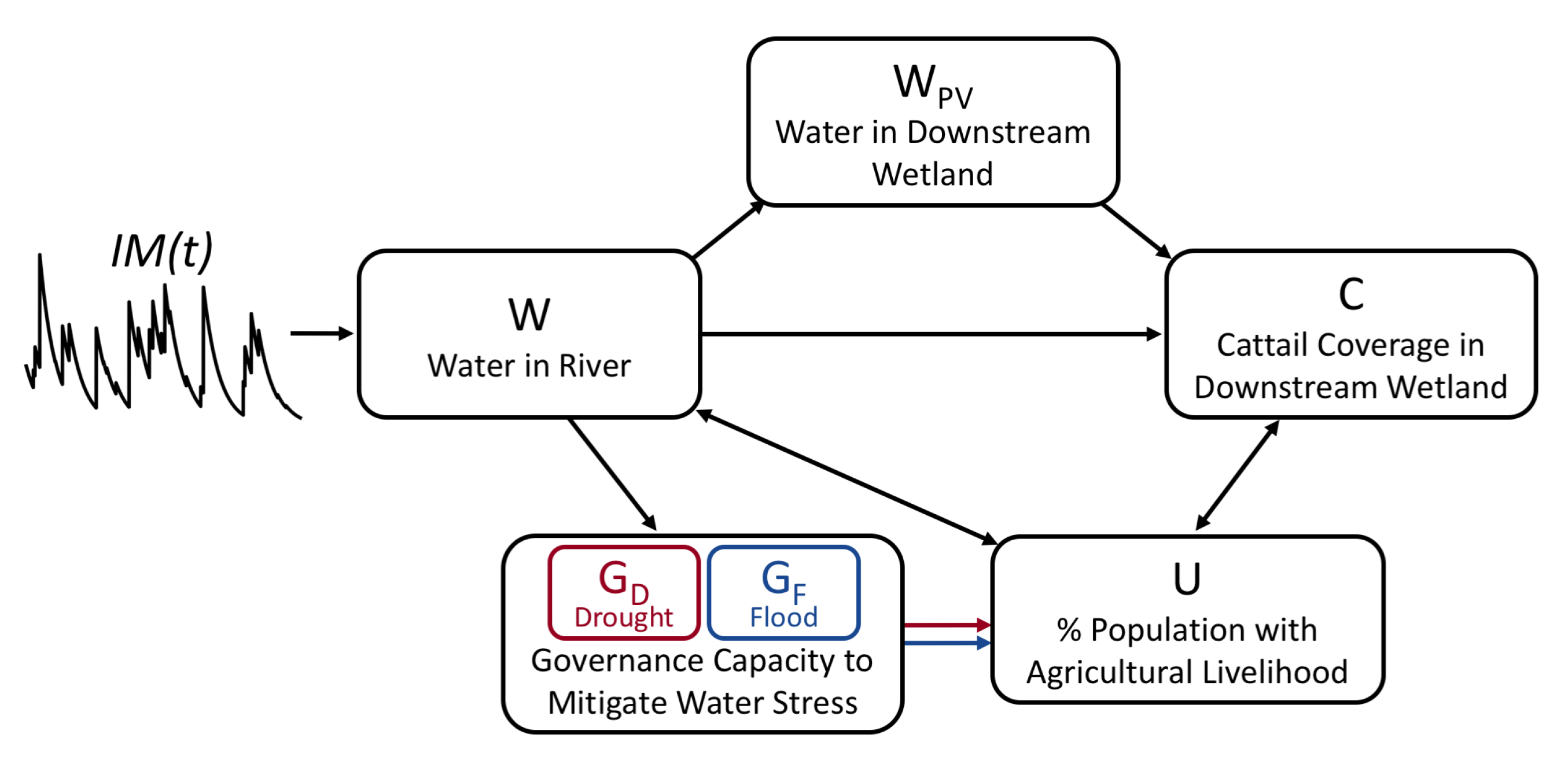
2.1. Model Structure

The model was developed with a goal of capturing the social and eco-hydrologic dynamics in a complex social-ecological system. The model focuses on a type of social-ecological system where human and environmental activities are strongly linked with the possibility for nonlinear dynamics. In this system, residents’ livelihoods come from either the agricultural sector or an alternative industry (e.g., tourism), local governance infrastructure reacts to extreme environmental conditions (e.g., flooding), all impacting a downstream wetland. Six dynamical variables were chosen accordingly, with three eco-hydrologic variables and three social variables, summarized in

Table 1. Dynamical variables and parameters of the model.

Symbol	Unit	Definition
Dynamical Variables
W	L${}^3$	Water in river
$W_{\mathit{PV}}$	L${}^3$	Water in downstream wetland
U	-	% of population participating in the agricultural sector
G	-	Governance capacity: the ability to mitigate adverse effects of drought
C	-	Cattail coverage as % of the wetland area
Parameters
$IM$	L${}^3$/T	Inflows of water, including the portion transferred/imported into the basin
$Ag$	1/NT	Per capita water allocation rate to farmers
$To$	1/T	Water allocation rate to alternative industry
q	1/T	Rate of water leaving the river and entering the wetland
$q^{\prime }$	1/T	Rate of water leaving the wetland
r	N/$	Population responsiveness to difference in profit
n	N	Population size in the system
${\pi }_T$	$/NT	Per capita income stream for people in alternative industry
${\pi }_A$	$/NT	Per capita income stream for people in the agricultural sector
p	$/(L${}^3$)${}^2$	Factor converting agricultural water allocation to profit
b	$/NT	Base per capita agricultural profit
c	L${}^3$/NT	Per capita farmer allocation threshold, below which drought occurs
f	L${}^3$	flood cutoff
D	1/T	Decay rate of governance capacity
$\beta$	-	% Damage by birds to agricultural products
$m_D$	N/L${}^3$	Rate of improvement of governance capacity dependent on severity of drought
$m_F$	1/TL${}^3$	Rate of improvement of governance capacity dependent on severity of flood
g	1/T	Natural growth rate of cattail
$g_A$	1/([M/L${}^3$]T)	Additional cattail growth rate induced by increased nutrient concentration due to agricultural activities
k	M/L${}^3$	Nutrient concentration in agricultural runoff
F	1/T	Rate of mechanical cattail removal

The symbols for unit/dimension are as follows: L for length; T for time; M for mass (e.g., mg of nutrients); N = number of people; $ for monetary unit.

and Figure 1 (see [11] for more details on dynamical variable selection). Water in the river (W) represents the available pool of water for industries and the environment. The amount of water ($W_{\mathit{PV}}$) and invasive cattail (C) in the downstream wetland indicate environmental health. The percent of the population with agricultural livelihoods (U) represents the persistence or collapse of the agricultural sector in the watershed. The water governance capacity indicates the ability of the institutional systems to provide assistance to farmers in times of drought ($G_D$) or flood ($G_F$). This model was built on a previous model [11] with the major modification being the inclusion of the negative impact of too much water (flooding) and the governance capacity to deal with flooding ($G_F$).

The dynamics of W and $W_{PV}$ reflect a simplified mass balance. Water enters the system and exits to the agricultural sector, alternative industry, and the wetland, $W_{PV}$. The growth of invasive cattail in the wetland, C, is increased by agricultural runoff (determined by W, U, and $W_{PV}$) and inhibited by management practices. Participation in the agricultural sector, U, is modeled using a replicator equation borrowed from evolutionary game theory [12]: people choose an agricultural livelihood when the payoff is better than the alternative industry. The payoff of agriculture depends on the state of the system: whether there is a flood or a drought (determined by W), whether there is the governance capacity to help when there is a flood or a drought ($G_F$ and $G_D$), and the severity of the degradation of the wetland (C). Both governance capacity variables, $G_F$ and $G_D$, operate on an assumption of institutional memory. When the system experiences an event (flood or drought), they gain experience and are thus better equipped to handle the next event that comes along. When an event does not occur for an extended period of time, the capacity drops. This dynamic was incorporated to explore how the frequency as well as magnitude of events can affect the system’s resilience. These dynamics are captured in Equations (1)–(6). (Further details can be found in Appendix A and Appendix B.)

$$\begin{array}{cc}\hfill \frac{dW}{dt}& =IM\left(t\right)-(Ag·n·U+To+q)·W\hfill \end{array}$$

(1)

$$\begin{array}{cc}\hfill \frac{d{W}_{PV}}{dt}& =q·W-q^{\prime }·W_{PV}\hfill \end{array}$$

(2)

$$\begin{array}{cc}\hfill \frac{dC}{dt}& =\left(g+\frac{Ag·n·U·W·k}{q^{\prime }·W_{PV}}·g_A\right)·C·(1-C)-F\hfill \end{array}$$

(3)

$$\begin{array}{cc}\hfill \frac{d{G}_D}{dt}& =I_{Ag·W<c}·m_D·(c-Ag·W)·(1-G_D)-D·G_D\hfill \end{array}$$

(4)

$$\begin{array}{cc}\hfill \frac{d{G}_F}{dt}& =I_{W>f}·m_F·(W-f)·(1-G_F)-D·G_F\hfill \end{array}$$

(5)

$$\begin{array}{cc}\hfill \frac{dU}{dt}& =r·U·(1-U)({\pi }_A-{\pi }_T)\hfill \end{array}$$

(6)

where,

$${\pi }_A=[p(1-G^{\prime })(Ag·W-c)(f-W)+b](1-\beta C)$$

$$G^{\prime }=\left\{\begin{array}{cc}{G}_D\hfill & \mathrm{if}Ag·W<c\hfill \\ G_F\hfill & \mathrm{if}W>f\hfill \\ 0\hfill & \mathrm{otw}.\hfill \end{array}\right.$$

2.2. Introducing Variable Water Availability

To investigate system resilience under environmental variability, we incorporated the stochasticity of the incoming water, $IM\left(t\right)$. This is a key modification: In the previous deterministic model [11], the incoming water was a constant parameter. For any one value of this parameter, there could be only one model outcome. In this work, incoming water is a stochastic dynamical variable. With the addition of stochasticity, we are able to explore how a single mean value can produce different model outcomes depending on the nature of the fluctuations. To model variations in incoming water, we considered a suite of marked Poisson $IM\left(t\right)$. A marked Poisson model of incoming water has been used to capture hydrological fluctuation [13,14,15] while keeping the simplicity of the original model. To map the model outcomes, parameters of the marked Poisson process were varied to create incoming water signals with an array of frequency and amplitude. For each set of parameters, a marked Poisson process was used to generate $IM\left(t\right)$ and the model was run until it reached equilibrium—i.e., when the system no longer exhibited directional changes. This was repeated for 500 realizations. The model outcome of interest is the persistence or collapse of the agricultural sector as defined by a collapse cutoff. When the participation in agriculture (U) was below a collapse cutoff of 2%, the sector was considered to have collapsed. The results, especially those associated with the flood-prone conditions, are quite robust against reasonable choices of the cutoff values (low values to define a collapse). For each parameter set, the percent of the 500 realizations where the agricultural sector collapsed was mapped. To explore the effect of drought-prone and flood-prone conditions, this process was repeated for a range of mean incoming water values, each resulting in a model outcome map (Figure 2). These resilience–amplitude–frequency maps help us understand how both changes in the mean water availability and changes in the occurrence and severity of extreme events can influence how regime shifts occur.

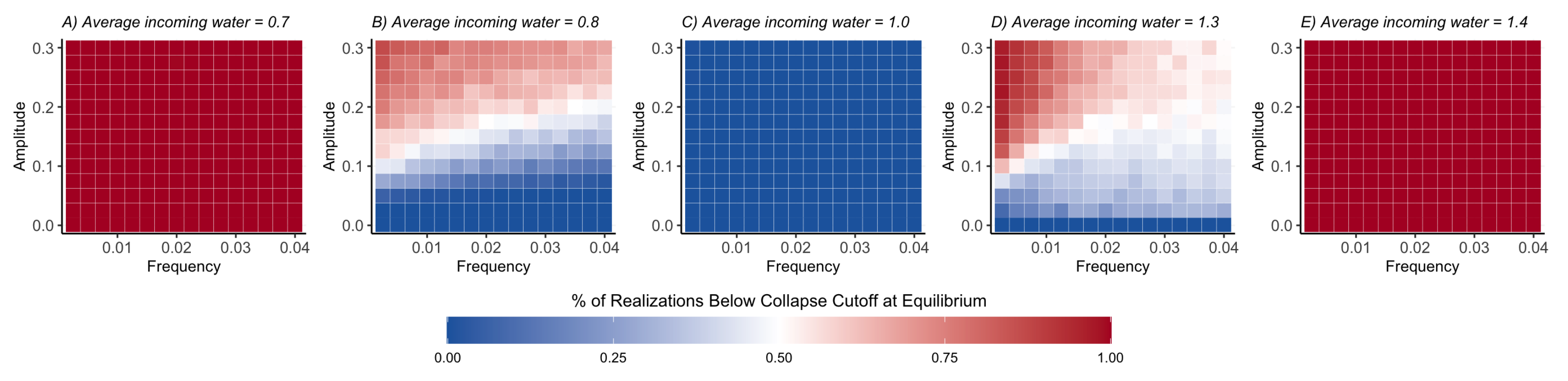
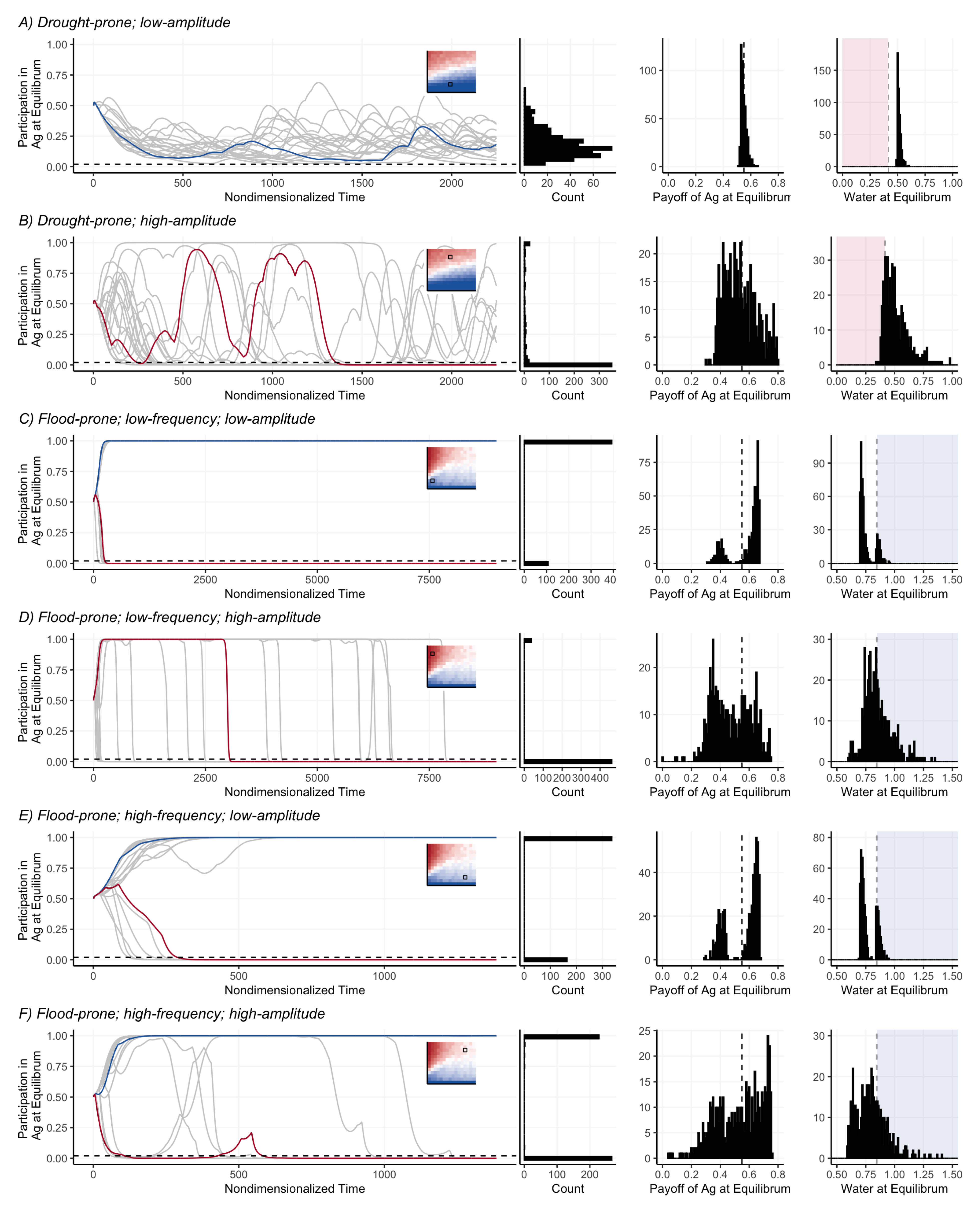
3. Results and Discussion

Figure 2 includes model results associated with a value of amplitude close to zero, representing the model outcome without fluctuation: These results represent “deterministic benchmarks” that highlight the effects of the environmental variation. In this deterministic case, the agricultural sector survives the mean incoming water in Figure 2B–D. Without taking environmental variation into account, the model overestimates the ability of the system to withstand changes in incoming water—Figure 2B,D allows us to explore system dynamics that would otherwise be overlooked in a deterministic model.

Under drought-prone conditions, the transition from agricultural sector survival to collapse is gradual and largely dependent on the amplitude of variation, with the system surviving low-amplitude variation at any frequency (Figure 2B). The histogram of W (Figure 3A, rightmost panel) is highly concentrated at a value near, but above, the drought cutoff. These values of W correspond to an agriculture payoff competitive with the payoff of alternative industry. When the payoff to agriculture fluctuates between being the more profitable option and the less profitable option, it drives fluctuations in U. The time series of U accordingly fluctuates near, but above, collapse.

Increasing the amplitude (comparing Figure 3B to Figure 3A) resulted in a more dispersed histogram of W, with some values falling below the drought cutoff. The histogram of U exhibits a dramatic shift: it is no longer concentrated around a mean; rather it becomes bimodal, with the primary peak at $U=0$. While the histogram of U in this case (Figure 3B, second panel from left) may appear similar to those in Figure 3C–F, it is important to note that a mixed strategy ($0<U<1$) is still possible, even with a peak at $U=0$; that is, there are some, although relatively few, realizations with U in the intermediate range. This is not the case with a flood-prone system.

When a drought occurs, the payoff of agriculture becomes less appealing than alternative employment, driving U towards 0. Due to the replicator dynamics of U, the more time U spends approaching 0, the harder it becomes to recover. The higher the amplitude of variation, the more likely it is that the system will encounter a drought. The more time the system spends in a drought, the more likely it is for the agricultural sector to collapse. This leads to the gradient from survival to collapse along the amplitude dimension seen in Figure 2B.

The frequency of variation affects how much time the system has to respond to fluctuations. High frequency oscillations move quickly with respect to other processes, meaning that if a drought occurs, the system may not have time to fully collapse before the drought ends and conditions become more favorable. Low frequency oscillations subject the system to water stress for a more extended period of time. A minor drought that lasts longer gives U more time to decline towards 0, eventually leading to a collapse of the agricultural sector. This means a lower amplitude of variation is needed to cause a system collapse when the frequency is low, which can be seen in Figure 2B.

Frequency plays a bigger role in the transition to collapse under flood-prone conditions (Figure 2D). At lower frequencies, the system experiences either near complete survival (the percentage of realizations below the collapse cutoff is near 0%) or near complete collapse (near 100% below collapse cutoff), with a very sharp transition between the two (compared to the transition under drought-prone conditions). At higher frequencies, the transition is much more gradual and moves between less extreme states. Additionally, from the time series and histograms of U in Figure 3C–F, we see that U demonstrates bimodal behavior under flood-prone conditions. Under any frequency and amplitude, participation in agriculture at equilibrium is concentrated near 0% and 100%.

With low-amplitude variation (Figure 3C,E), the histograms of W display a bimodal distribution—W can be concentrated above or below the flood cutoff. In other words, the system can move to either a flooding or non-flooding regime. When the system moves to a flooding regime, the payoff to agriculture is driven down, and vice versa. Unlike in the drought-prone case, the payoff to agriculture is not fluctuating around the payoff to alternative industry in either flooding or non-flooding regime. Instead, the payoff is fluctuating entirely below or entirely above the payoff to alternative industry. Fluctuations fully below the alternative payoff will not result in fluctuations of U, but will affect how fast U collapses. The time series in Figure 3C and E highlight the “legacy effect”: where the system ends up at equilibrium (full collapse or full survival of the agricultural sector), depends on which path was taken at the outset: towards a flooding regime or towards a non-flooding regime.

Higher amplitude variation blurs the lines between flooding and non-flooding regimes: the histograms of W in Figure 3D,F do not display the strong bimodality seen in cases with low-amplitude variation. Higher amplitude variation allows transition between the two system states of collapse and survival. The time series in Figure 3D shows that even if agriculture reaches near full participation, the system can still collapse later on. In Figure 3F, the system can not only collapse later on, but can recover as well. Just as in the water shortage case, lower frequency oscillations subject the system to a more extended period of time with near 0% participation, making it increasingly harder for the system to recover. Higher frequency oscillations allow for more movement between the two alternatives, resulting in less extreme collapse and survival conditions.

4. Conclusions

Changes in the frequency and amplitude of environmental events can have serious impacts on the sustainability of social-ecological systems. In this paper, we asked: How do the frequency and amplitude of water availability variation affect both the social-ecological regimes present and how the system transitions between them? How do these transitions differ under flood-prone and drought-prone conditions? A dynamical systems approach allowed us to explore the qualitative behavior of the system under different conditions, rather than predict the outcome of a particular system. Our analysis resulted in a more systematic framework to investigate the linkages between sustainability of social-ecological systems and environmental variability, e.g., the resilience–amplitude–frequency maps. These maps allowed us to examine system dynamics that would be missed using a deterministic model.

In both flood- and drought- prone systems, resilience was overestimated when variation was not considered. We found that survival or collapse of the agricultural sector is largely determined by the magnitude of the events. Under both flood- and drought-prone conditions, the system survives frequent events better than infrequent, but prolonged, unfavorable conditions. Agricultural sector collapse due to water shortage happens more gradually, with the possibility for a mix of livelihoods. Collapse of the agricultural sector due to water surplus, however, happens more suddenly, and without the possibility of a mix of livelihoods—once conditions become severe enough, the system transitions from fully agricultural to full abandonment.

The frequency of flooding events was found to be more impactful than the frequency of drought events. The agricultural sector could still bounce back after collapse caused by more frequent flooding, whereas less frequent, but longer flooding episodes will lead to a more permanent collapse of the agricultural sector. Low-amplitude variation does not facilitate much transition between the two system outcomes, whereas higher amplitude, higher frequency variation allows the system to move back and forth. High amplitude, low frequency variation allows the system to move from survival to collapse, but it is more difficult to move back once flooding is established.

Incorporating stochastic environmental variation into a dynamical model of a social-ecological system allowed us to directly link the frequencies and severity of environmental events (water surplus and shortage) to system-level outcomes (livelihood choices) in a systematic and quantitative way. This direct link can be difficult to achieve with more highly-parameterized models. Stylized dynamical systems models such as this offer a different perspective on complex problems, with potential to be adapted to similarly interconnected social-ecological systems. Insights and lessons from this approach may be applied to a range of future research, including model development with the goal of predicting social-ecological outcomes. This lays groundwork for future research in systems with significant current or predicted environmental variability due to climate change.

References

1. Aghakouchak, A.; Chiang, F.; Huning, L.S.; Love, C.A.; Mallakpour, I.; Mazdiyasni, O.; Moftakhari, H.; Papalexiou, S.M.; Ragno, E.; Sadegh, M. Climate Extremes and Compound Hazards in a Warming World. Annu. Rev. Earth Planet. Sci. 2020, 48, 519–548. [Google Scholar] [CrossRef] [Green Version]
2. Guttal, V.; Jayaprakash, C. Impact of noise on bistable ecological systems. Ecol. Model. 2007, 201, 420–428. [Google Scholar] [CrossRef]
3. Borgogno, F.; D’Odorico, P.; Laio, F.; Ridolfi, L. Effect of rainfall interannual variability on the stability and resilience of dryland plant ecosystems. Water Resour. Res. 2007, 43. [Google Scholar] [CrossRef]
4. Xu, L.; Patterson, D.; Staver, A.C.; Levin, S.A.; Wang, J. Unifying deterministic and stochastic ecological dynamics via a landscape-flux approach. Proc. Natl. Acad. Sci. USA 2021, 118, e2103779118. [Google Scholar] [CrossRef] [PubMed]
5. Virapongse, A.; Brooks, S.; Metcalf, E.C.; Zedalis, M.; Gosz, J.; Kliskey, A.; Alessa, L. A social-ecological systems approach for environmental management. J. Environ. Manag. 2016, 178, 83–91. [Google Scholar] [CrossRef] [PubMed] [Green Version]
6. Biggs, R.; Schlüter, M.; Biggs, D.; Bohensky, E.L.; Burnsilver, S.; Cundill, G.; Dakos, V.; Daw, T.M.; Evans, L.S.; Kotschy, K.; et al. Toward principles for enhancing the resilience of ecosystem services. Annu. Rev. Environ. Resour. 2012, 37, 421–448. [Google Scholar] [CrossRef] [Green Version]
7. Linstädter, A.; Kuhn, A.; Naumann, C.; Rasch, S.; Sandhage-Hofmann, A.; Amelung, W.; Jordaan, J.; Du Preez, C.C.; Bollig, M. Assessing the resilience of a real-world social-ecological system: Lessons from a multidisciplinary evaluation of a South African pastoral system. Ecol. Soc. 2016, 21. [Google Scholar] [CrossRef] [Green Version]
8. Nemec, K.T.; Chan, J.; Hoffman, C.; Spanbauer, T.L.; Hamm, J.A.; Allen, C.R.; Hefley, T.; Pan, D.; Shrestha, P. Assessing resilience in stressed watersheds. Ecol. Soc. 2014, 19. [Google Scholar] [CrossRef] [Green Version]
9. Lamichhane, P.; Miller, K.K.; Hadjikakou, M.; Bryan, B.A. Resilience of smallholder cropping to climatic variability. Sci. Total. Environ. 2020, 719, 137464. [Google Scholar] [CrossRef] [PubMed]
10. Liu, D. Evaluating the dynamic resilience process of a regional water resource system through the nexus approach and resilience routing analysis. J. Hydrol. 2019, 578, 124028. [Google Scholar] [CrossRef]
11. Vazquez, K.; Muneepeerakul, R. Modeling resilience and sustainability of water-subsidized systems: An example from northwest Costa Rica. Sustainability 2021, 13, 2013. [Google Scholar] [CrossRef]
12. Nowak, M.A. Evolutionary Dynamics: Exploring the Equations of Life; Harvard University Press: Chicago, IL, USA, 2006. [Google Scholar]
13. Botter, G.; Porporato, A.; Rodriguez-Iturbe, I.; Rinaldo, A. Basin-scale soil moisture dynamics and the probabilistic characterization of carrier hydrologic flows: Slow, leaching-prone components of the hydrologic response. Water Resour. Res. 2007, 43. [Google Scholar] [CrossRef]
14. Porporato, A.; Daly, E.; Rodriguez-Iturbe, I. Soil water balance and ecosystem response to climate change. Am. Nat. 2004, 164, 625–632. [Google Scholar] [CrossRef] [PubMed]
15. Rodriguez-Iturbe, I.; Porporato, A.; Rldolfi, L.; Isham, V.; Cox, D.R. Probabilistic modelling of water balance at a point: The role of climate, soil and vegetation. Proc. R. Soc. A Math. Phys. Eng. Sci. 1999, 455, 3789–3805. [Google Scholar] [CrossRef]
16. Guzmán Arias, I.; Calvo Alvarado, J.C. Water resources of the Upper Tempisque River Watershed, Costa Rica ( Technical note). Tecnol. Marcha 2012, 25, 63–70. [Google Scholar]
17. Guzmán-Arias, I.; Calvo-Alvarado, J. Planning and development of Costa Rica water resources: Current status and perspectives. Tecnol. Marcha 2013, 26, 52–63. [Google Scholar] [CrossRef]
18. Osland, M.J.; González, E.; Richardson, C.J. Restoring diversity after cattail expansion: Disturbance, resilience, and seasonality in a tropical dry wetland. Ecol. Appl. 2011, 21, 715–728. [Google Scholar] [CrossRef] [PubMed] [Green Version]
19. Waylen, P.; Sadí Laporte, M. Flooding and the El Niño-Southern Oscillation phenomenon along the Pacific coast of Costa Rica. Hydrol. Process. 1999, 13, 2623–2638. [Google Scholar] [CrossRef]
Figure 1. A conceptual diagram of the model. Directed links represent causal effects from one dynamical variable to another. Dynamical variables G D and G F are distinct, but interact with the model in essentially the same way depending on if the system is experiencing drought or flood. I M ( t ) is the variable incoming water, modeled using a marked Poisson process.
Sustainability 14 01948 g001
Figure 2. Resilience–amplitude–frequency maps under different hydrological conditions, ranging from drought-prone to flood-prone. The color represents the fraction of realizations where the agricultural system collapsed at equilibrium. In (A,E), with too low or too high a mean value of I M ( t ) , the agricultural sector cannot support itself at any frequency or amplitude. Between these extremes (C), the system survives at all frequencies and intensities. The system transitions between these states of full collapse and full survival with different behavior depending on whether collapse is driven by a shortage of water (B) or a surplus of water (D).
Sustainability 14 01948 g002
Figure 3. Sample time series of U, and histograms of U, payoff to agriculture, and W values at equilibrium from 500 realizations under different hydrological conditions. The dashed line in the histograms of payoff to agriculture represents payoff to alternative industry—when payoff to agriculture is above this line, it is the more appealing livelihood option. In (A,B), the dashed line and change in color in the histograms of W represents the drought cutoff; in (CF), they represent the flood cutoff.
Sustainability 14 01948 g003