Optical Performance Comparison of Different Shapes of Cavity Receiver in the Fixed Line-Focus Solar Concentrating System

Abstract

To optimize the fixed-focus solar concentrating system (FLSCS) and linear cavity receiver of better optical performance, the effects of receiver parameters (geometric shape, receiver position f, receiver internal surface absorptivity α_ab, and end reflection plane reflectivity ρ_r) on the relative optical efficiency loss η_re-opt,loss, the maximum value of the local concentration ratio X_max, and the non-uniformity factor σ_non were studied in the present study. The results showed that the increases of sun declination angle δ in the range of 0–8° have a weak effect on the η_re-opt,loss. The η_re-opt,loss are 2.25%, 2.72%, 12.69% and 2.62%, 3.26%, 12.85%, respectively, when the solar hour angle ω is 0°, 30°, 60° as δ = 0° and 8° for linear rectangular cavity receiver. The X_max mainly depends on the energy flux distribution of first intercepted sunlight on the cavity absorber inner wall. Increasing the distance between the cavity absorber inner wall and the focal line Δf can affect the X_max. The smaller the Δf, the greater the X_max, and vice versa. The changing trend of σ_non is basically consistent with that of the X_max. When the f is 600, 625, 650, 675, 700 mm and the ω = 0°, the σ_non are 0.832, 0.828, 0.801, 0.747, and 0.671, respectively, for linear rectangular cavity receiver. This work could establish the foundation for further research on the optical to thermal energy conversion in the FLSCS.

1. Introduction

The technology of the concentrating solar collectors is promising for the solar heating system in residential housing [1,2]. The schematic of a concentrated solar heating system used to charge a storage tank of heat transfer fluid (HTF) is shown in Figure 1. Solar energy is harnessed in a fixed line-focus solar concentrating system (FLSCS) at a higher relative temperature compared to the ambient. It is utilized to heat the HTF in the cavity receiver. Note that the FLSCS can provide a relatively high optical efficiency for a whole year running based on the lens element’s simple periodic slip adjustment [3,4]. The cavity receiver is fixedly installed in the system, which causes its structural parameters to have a significant impact on the system’s optical performance during the sun-tracking process of the solar concentrator.

In the literature, diverse works on cavity receivers have been performed by many researchers to improve the performance of solar concentrating systems. Patil et al. [5] reported a 5 kW solar cavity receiver containing a reticulated porous ceramic structure. The results showed that the system achieved a peak efficiency of 0.69 at 1133 °C air outlet temperature. Liang et al. [6] presented a cavity receiver consisting of a centre tube and two inclined fins for the parabolic trough solar collector (PTC). It was found that the experimental collector efficiency was in the range of 34.18–48.57%. Liang et al. [7] also studied the effects of the movable cover on reducing heat loss and overheating protection of a cavity receiver for PTC. They concluded that the heat loss reduction rate varied from 6.36% to 13.55% when turning off the movable cover was applied. Ebrahimpour et al. [8] investigated the influence of radiation and convection modes on the behavior of air for linear Fresnel reflector (LFR) with trapezoidal cavity receiver. Temperature difference augments about 180% when adiabatic wall angle enhances as temperature ratio is 0.8. Alipourtarzanagh et al. [9] analyzed the mechanism of heat losses from a cylindrical solar cavity receiver equipped with an air curtain. It was found that increasing the air curtain speed can reduce heat loss by up to 60% when the air curtain discharge angle is 30°. Fang et al. [10] described the influence of surface optical and radiative properties on the thermal performance of a solar cavity receiver. The results indicated that the receiver efficiency is enhanced by about 12.6% as the solar absorptivity rises from 0.8 to 1.0. Li et al. [11] proposed a major arc-shaped linear cavity receiver with a lunate channel based on parabolic trough solar collectors’ black cavity effect principle. The results show that it has a comparable or even better performance compared with evacuated tube collectors. Abbasi-Shavazi et al. [12] examined experimentally the heat loss from a model solar cavity receiver. The results show that the concept of stagnation and convection zone development in cavities are consistent with increasing cavity inclination angle.

In addition, many researchers have analyzed the influence of cavity receiver parameters on the system’s optical performance. Lin et al. [13] proposed and studied a linear Fresnel lens collector with four types of cavity receivers using east–west horizontal tracking mode. The analysis confirms that the Fresnel lens solar collector with triangular cavity receiver boasts best performance in terms of both optical and thermal characteristics. Sedighi et al. [14] proposed an indirectly irradiated cavity receiver. According to the result, a cylindrical cavity with an inverted conical base provides the highest optical efficiency, around 92%, compared to other cylindrical cavities with different base shapes. Sumit et al. [15] studied the performance of a tapered helical coil solar receiver with a nanostructured carbon florets coating. The efficiency increases from 48.4% to 68% for a closed cavity receiver at a flow rate of 20 L/min on the application of thermal coating. Abuseada et al. [16] surveyed a cavity receiver’s energy-efficient variable aperture mechanism. The result indicated that the aperture blades captured 54% of intercepted surplus power. Slootweg et al. [17] presented a complex geometry solar tower molten salt cavity receiver and investigated its optical and thermal performance. It was found that optical efficiencies of the cavity receiver reached efficiencies over 93%. Soltani et al. [18] studied a helically baffled cylindrical cavity receiver in a parabolic dish collector. The results show that the performance can enhance up to 65% by selecting effective parameters. Aslfattahi et al. [19] evaluated the solar dish collector for three cavity receivers: cubical, hemispherical, and cylindrical shapes. According to the analysis, the hemispherical cavity receiver led to maximum thermal efficiency with the nanofluid used. Wang et al. [20,21] investigated the effects of receiver parameters on the optical performance of a Fresnel lens solar system. The analysis shows that average optical efficiencies using cavity receiver with the bottom reflective cone of spherical, cylindrical, and conical are 72.23%, 68.37%, and 76.40%, respectively. Lee et al. [22] assessed the effect of aspect ratio and head-on wind speed on the force and natural convective heat loss and area-averaged convective heat flux from a cylindrical solar cavity receiver. The numerical analysis indicates that the overall efficiency of the solar cavity receiver increases with the aspect ratio. Tu et al. [23] studied the effects of radiative surface properties inside a solar cavity receiver. They found that both the radiative and the convective heat loss of the present cavity receiver decrease with increasing thermal emissivity and improves the receiver’s efficiency.

The literature shows that the study has been conducted extensively on cavity receivers for the concentrating solar collectors. However, there is no research on the comparative analysis of different shapes of linear cavity receivers used in fixed-focus solar concentrating systems in the published literature. Linear cavity receivers of various shapes provide different sunlight interception capabilities and form different energy flux distributions due to their design. Therefore, this work aims to investigate optical performance comparison of different shapes of cavity receivers in the FLSCS, which has not been reported earlier in the literature. The investigation of the optical performance comparison of different shapes of cavity receivers helps in understanding (a) the efficacy of the various shapes of cavity receiver design and (b) the optical behaviour of the receiver internal surface absorptivity and end reflection plane reflectivity on the receiver losses.

In this study, to optimize the FLSCS and linear cavity receiver of better optical performance, the present study concentrates on the effects of receiver parameters (geometric shape, receiver position f, receiver internal surface absorptivity α_ab, and end reflection plane reflectivity ρ_r) on the optical efficiency of system and flux uniformity of linear cavity receiver. This work could provide a reference for the design and optimization of the optical matching between the fixed line-focus solar concentrator and linear cavity receiver and established the foundation for further research on the optical to thermal energy conversion in the FLSCS.

2. Physical Model and Numerical Method

2.1. Physical Model

The FLSCS is shown schematically in Figure 1. The parameters include the lens element length L, lens element width B of linear Fresnel lens and receiver position f, sun declination angle δ, solar hour angle ω, sunlight incidence angle θ and latitude angle φ. The linear Fresnel lens concentrates sunlight into the fixed linear cavity receiver through the polar tracking system. The polar axis of FLSCS is aligned parallel with that of the earth. The lens element slides on the lens frame according to the change of δ to ensure that the focal line does not exceed the end of the fixed linear cavity receiver. The incident sunlight is completely intercepted by the opening plane of the fixed linear cavity receiver under ideal conditions. The horizontal angle of the polar-axis depends on the φ. For daily tracking, linear Fresnel lens rotates around the polar-axis from east to west every day at the earth rotation angular velocity with the help of a driving motor. For seasonal tracking, the linear Fresnel lens manually adjusts at δ with the use of the lens frame. The working fluid flows in from the lower side of the cavity and flows out from the higher side, thereby taking away the heat. Heat transfer oil is used as the heat transfer working medium. The model and methodology can be extrapolated in other countries by modifying the design parameters and operating conditions.

According to the previous work of our team [3,4], the θ in FLSCS shown in Figure 1, is determined by the following formula:

$$\cos \theta =\sin \delta \sin (\phi -S)+\cos \delta \cos (\phi -S)\cos \omega$$

(1)

The S is the horizontal angle of the polar axis, and the S = φ. In addition, the ω = 0° under ideal tracking conditions. Applying them for Formula (1), we have:

$$\cos \theta =\cos \delta$$

(2)

Moreover, the δ can be expressed as [24,25],

$$\delta =23.45°\times \sin [\frac{360}{365}(284+N)]$$

(3)

The N is the day number of the year with N = 1 on 1 January.

2.2. Numerical Simulation Model

To estimate the optical performance of linear cavity receiver in the FLSCS, commercial software TracePro^® using the Monte Carlo ray tracing method was applied. Figure 2a displays the FLSCS system using one of the modelled receivers, linear triangular cavity receiver (LTCR), through the ray-tracing analysis. The incident sunlight is concentrated by the linear Fresnel lens, then intercepted and absorbed by the LTCR, and part of the sunlight escapes after being reflected. Figure 2b shows the energy flux distribution in the LTCR. The energy flux is mainly distributed at the bottom of the LTCR, and the energy flux density shows non-uniform characteristics.

The receivers used in this study are LTCR, linear arc-shaped cavity receiver (LACR), and linear rectangular cavity receiver (LRCR). Moreover, three shapes of the linear cavity receiver are composed of coated copper tubes through which heat transfer fluid flows, as shown in Figure 3. All cavity receivers’ opening size and internal surface area are the same, as shown in

Table 1. Parameters of FLSCS using linear cavity receiver for comparison.

Component	Parameter	Symbol	Value
Linear Fresnel lens	Lens element width	B	400 mm
	Lens element length	L	1500 mm
	Focal length	f0	650 mm
	Thickness	t	2 mm
	Prism size	p	0.1 mm
LTCR	Opening width	Btr	80 mm
	Opening length	Ltr	1500 mm
	Apex angle	αtr	60°
LACR	Opening width	Bar	80 mm
	Opening length	Lar	1500 mm
	Diameter	Dar	84.43 mm
LRCR	Opening width	Bre	80 mm
	Opening length	Lre	1500 mm
	Height	Hre	40 mm

.

The optical performance comparison of different shapes of linear cavity receivers in the FLSCS is carried out under ideal conditions. Therefore, engineering errors are not considered, including the slope, specular, and contour errors of a linear Fresnel lens, the installation error of the linear cavity receiver, the system’s tracking error, etc. [26,27]. The half angular width of the sun is set to 0.27° during simulation to close to reality [28,29].

2.3. Optical Work Validation

The proposed method carried out in this research has been validated against the experimental work in our previous works [3,4], see Figure 4. After designing an optical model and setting up the TracePro^® software, the results of both works were compared, and a good agreement was achieved. According to the experimental and simulated results, the maximum flux density on the Lambert board is 18,137 W/m² and 19,052 W/m², when the direct solar irradiance I_d is 796 W/m² at 2:50 pm 29 July 2020. The main facula relative error between the filling area S₀ under the experimental curves and the S_0′ under the simulated curves is 3.24%. The relative error between the filling area S₁ under the experimental curves and the S_1′ under the simulated curves is 15.35%.

2.4. Optical Analysis

Since the photothermal conversion takes place on the internal wall of the linear cavity receiver, the optical efficiency of the FLSCS (η_opt) can be described by Formula (4) [30,31]:

$${\eta }_{opt}=\frac{Q_{absorber}}{B\cdot L\cdot I_d\cdot \cos \theta }=\frac{A_{absorber}\cdot G_{mean}}{B\cdot L\cdot I_d\cdot \cos \theta }=\frac{A_{absorber}}{B\cdot L\cdot \cos \theta \cdot X_{mean}}$$

(4)

where Q_absorber (W) is the sunlight energy absorbed by the internal wall of the linear cavity receiver, A_absorber (m²) is the total area of the internal surface, G_mean (W/m²) is the average flux density on the absorber, and X_mean is the mean value of the local energy flux concentration ratio. To facilitate comparison and avoid being affected by the cosine effect of the θ, the relative optical efficiency loss (η_re-opt,loss) is used to estimate the effects of receiver parameters on the optical efficiency of the FLSCS. η_re-opt,loss of the system can be calculated by:

$${\eta }_{re-opt,loss}=\frac{Q_{absorber,ref}-Q_{absorber,\delta ,\omega }}{Q_{absorber,ref}}$$

(5)

where Q_{absorber,δ,ω} (W) is the sunlight energy absorbed by the internal wall of the linear cavity receiver when the sun declination angle and solar hour angle is δ and ω, respectively. Q_absorber,ref (W) is the sunlight energy absorbed by the internal wall of the liner cavity receiver when the sun declination angle and solar hour angle are 0°, receiver internal surface absorptivity and end reflection plane reflectivity are 1.00 and receiver position is 650 mm. The mean value X_mean and maximum value X_max of the local concentration ratio of the energy flux are simply obtained by applying Formulas (5) and (6), respectively [32,33]:

$$X_{mean}=\frac{G_{mean}}{I_d}$$

(6)

$$X_{max}=\frac{G_{max}}{I_d}$$

(7)

where G_max (W/m²) is the maximum energy flux density, respectively. For comparison, the flux uniformity of the receiver internal surface is defined by a non-uniformity factor (σ_non) as indicated below [34,35],

$${\sigma }_{\mathrm{non}}=\frac{X_{max}-X_{mean}}{X_{max}}$$

(8)

3. Results and Discussion

To investigate the optical performance of different shapes of linear cavity receivers in the FLSCS, we studied the optical efficiency of the solar system and the energy flux distribution in linear cavity receivers under different receiver parameters. Three various shapes of linear cavity receiver—LTCR, LACR, and LRCR—were studied (see Figure 3 and Table 1). The results were compared, which were obtained through simulation realized by the use of TracePro^® on different the f, θ, α_ab, and ρ_r. Cases differ in the η_re-opt,loss, X_max, and σ_non, allowing us to elucidate sensitivity analysis of the effective parameters in a linear cavity receiver. Essentially, the linear cavity receivers have the same area of internal wall and same size of the opening, but different shapes.

3.1. Effect of the Sunlight Incident Angle θ

To study the induced propagation and collection process of sunlight changes by the effect of the θ, we compare the optical performance index of the system when the δ is 0°, 8°, 16°, and 23.45° respectively, simulated under the f = 650 mm, α_ab = 0.85 and ρ_r = 0.85. In sun tracking, the change of the ω will also affect the propagation and collection of sunlight inside the cavity absorber. To monitor the optical performance index changes of the system during the sun tracking, we simulated the case of different ω and different δ.

Figure 5a shows the effect of the θ on the optical performance of the FLSCS using LTCR. The η_re-opt,loss is basically unchanged for ω of 0–30° and linearly increases for ω of 30–60°, when the δ = 0°. The η_re-opt,loss are 2.25%, 2.72%, and 12.69%, respectively, when the ω is 0°, 30°, 60°. A similar change in the η_re-opt,loss can be seen in Figure 5a, when the δ = 8°. Noted that the η_re-opt,loss are 2.62%, 3.26%, and 12.85%, respectively, when the ω is 0°, 30°, and 60°. It means that the increases of δ in the range of 0–8° have a weak effect on the η_re-opt,loss. However, as shown in Figure 5a, when the δ is 16° and 23.45°, the η_re-opt,loss increases as ω raises in the range of 0–60°, and the rate of increase becomes ever larger. When the δ is 16° and 23.45° and the ω is 0°, 30°, and 60°, the η_re-opt,loss are 2.94%, 4.69%, 23.1% and 4.68%, 14.43%, 41.73%, respectively. The maximum η_re-opt,loss of the latter is basically twice that of the former. It is mainly due to the upward movement of the focus line as the ω increases. Figure 6 shows the upward movement distance of the focal line with the θ. It can be seen that the focal line moves slowly upward for δ of 0–8° and rises sharply for δ of 8–23.45°.

To clearly observe the influence of the δ and ω on the propagation of sunlight, we analyze the propagation of sunlight within twice-intercepted by the cavity absorber through the simple diagram in Figure 7. The upward movement distance for δ = 8° is 10.7 mm, and the analysis is carried out with reference to Figure 7d–i. It reveals that the sunlight did not escape during the two interception processes of the cavity absorber for ω of 0–30°. Still, part of the first reflected sunlight escapes from the cavity absorber after ω = 30°, when δ is in the range of 0–8°. The upward movement distance for δ = 16° is 46.7 mm, and the analysis is carried out with reference to Figure 7a–c. It is inferred that part of the first reflected sunlight escapes from the cavity absorber for ω of 30–60° and even part of the incident sunlight fails to be intercepted by the cavity absorber and escapes directly as ω = 60°. The number of escaped first reflected sunlight increases with the increasing of ω and δ for δ of 16–23.45°. Therefore, in addition to the cosine loss caused by the δ, the existence of the above-mentioned escape sunlight exacerbates the increase in the η_re-opt,loss.

Moreover, as shown in Figure 5a, the X_max is increasing for ω of 0–60°, but the growth rate of X_max decreases for δ of 0–23.45°. The X_max mainly depends on the energy flux distribution of first intercepted sunlight on the cavity absorber inner wall. The symmetry plane of the linear Fresnel lens and the cavity receiver inner wall form an intersection line, and Δf represents the distance between the intersection line and the focal line. The energy flux distribution of the focus facula shows that the energy flux density in the main facula is much higher than that in the side facula [3,4]. The energy flux density of the focus facula is negatively related to the distance between the focal plane and the focal line. Therefore, Δf is used to describe the change process of the X_max intuitively. The smaller the Δf, the greater the energy flux density value on the intersection line, the greater the X_max, and vice versa. It can be seen in Figure 7a–i that when the δ is a fixed value, the Δf decreases with the increase of ω, increasing the X_max. With the increasing of δ, the focal line moves upward, and the Δf increases, finally leading to a decrease in the growth trend of Δf for ω of 0–60°, leading to a decline in the growth trend of the X_max. In addition, the X_max decreases with the increase of δ, when the ω is a constant value. For example, when the δ is 0°, 8°, 16° and 23.45° and the ω = 60°, the X_max are 6.461, 5.950, 4.428, and 2.773, respectively. This means that the δ has a greater influence than the ω on the X_max. In other words, the X_max can be reduced by moving the focal line upward. Furthermore, as shown in Figure 5a, the σ_non is increasing for ω of 0–60°. However, it can be seen in Figure 7a–i that the distribution area of the twice-intercepted sunlight does not monotonously increase or decrease with the change of ω. This means that the X_max is far greater than the X_mean, thus the σ_non mainly depends on the X_max. Note that the growth rate of σ_non increases for δ of 0–23.45°, while the X_max is the opposite. In addition, the σ_non decreases with the increase of δ, when the ω is a constant value. For example, when the δ is 0°, 8°, 16°, and 23.45° and the ω = 60°, the σ_non are 0.737, 0.715, 0.662, and 0.591, respectively. It indicates that the rate of escaped sunlight increases for δ of 0–23.45°, resulting in a sharp drop in the X_mean. It is consistent with the change of η_re-opt,loss. Analysis showed that the influence of δ on optical performance is extremely greater than that of ω.

As in the case of the LTCR, Figure 5b shows the effect of θ on the optical performance of the FLSCS using LACR. As shown in Figure 5b, the η_re-opt,loss decrease slowly for ω of 0–15° and decreases significantly for ω of 15–60°, when the δ = 0°. The η_re-opt,loss are 14.99%, 14.72%, and 2.61%, respectively, when the ω is 0°, 15°, and 60°. Referring to Figure 8g–i, the first intercepted sunlight escapes completely after being reflected as ω = 0°. After that, part of the first reflected sunlight is intercepted for the second time by the cavity absorber and the number of second intercepted sunlight also increases with the ω. A similar change in the η_re-opt,loss can be seen in Figure 5b, when the δ = 8°. Noted that the η_re-opt,loss is 15.12%, 14.33%, and 3.89%, respectively, when the ω is 0°, 15°, and 60°. This means that the increase of δ in the range of 0–8° has a weak effect on the η_re-opt,loss.

However, the η_re-opt,loss decreases for ω of 0–45° and increases for ω of 45–60° when the δ = 16°, as shown in Figure 5b. When the ω is 0°, 45°, and 60°, the η_re-opt,loss is 12.20%, 9.28%, and 18.03%, respectively. Referring to Figure 8a–c, part of the first reflected sunlight escapes after being reflected as ω = 0°. After that increases with the ω, the number of escaped first reflected sunlight decreases, but part of the incident sunlight is blocked by the cavity absorber, increasing optical loss. It is worth noting that the η_re-opt,loss increases for ω of 0–60° and the growth rate of η_re-opt,loss increases with ω, when the δ = 23.45°, as shown in Figure 5b. The η_re-opt,loss is 10.19%, 17.48%, and 40.53%, respectively, when the ω = 0°, 30°, 60°. Referring to Figure 8a–i, it can be inferred that the upward movement distance of the focal line is 97.2 mm as δ = 23.45°, causing the incident sunlight not to be completely intercepted by the cavity absorber and escape. With the increasing of ω, the number of escaped incident sunlight increases. This means that the η_re-opt,loss mainly depends on the first intercepted sunlight.

Moreover, as shown in Figure 5b, the X_max increases for ω of 0–45° but decreases for ω of 45–60°. Referring to Figure 8a–i, it can be seen that the Δf decreases during the tracking of ω, increasing the X_max of the energy flux distribution of the first intercepted sunlight. The secondary intercepted sunlight is reflected again to the distribution area of the first intercepted sunlight, resulting in the X_max being further increased for ω of 0–45°. However, the distribution area of the third intercepted sunlight gradually deviates from that of the first intercepted sunlight for ω of 45–60°, which can cause the X_max to decrease. Even though the focal line continues to approach the cavity absorber inner wall during the tracking of ω and the X_max increases, it is not enough to compensate for the decrease in the X_max caused by the deviation of the secondary reflected sunlight, which ultimately leads to a decrease in the X_max. The X_max mainly depends on the energy flux distribution of first intercepted sunlight, but the energy flux distribution of the subsequently intercepted sunlight can also affect the X_max.

Furthermore, as shown in Figure 5b, the σ_non increases for ω of 0–45° and decreases for ω of 45–60° when δ = 0° and 8°, which is similar to the change in the X_max. However, it can be seen in Figure 8d–i that the distribution area of the twice-intercepted sunlight increased for ω of 0–60°. This means that the X_max is far greater than the X_mean, thus the σ_non mainly depends on the X_max. Noted that the σ_non increases for ω of 0–60° when δ = 16° and 23.45°, as shown in Figure 5b, which is different from the previous two cases. The growth rate of σ_non increases for δ of 16–23.45°. It can be seen in Figure 8c that part of the incident sunlight failed to be intercepted by the cavity absorber for the first time as ω = 60°, resulting in a decrease in the X_mean. The X_max and σ_non decrease and increase respectively for ω of 45–60°, which means that the incident sunlight failed to be intercepted by the cavity absorber has a greater impact on the X_mean than the X_max. As the δ increases, the number of incident sunlight that fails to be intercepted by the cavity absorber increases, making the effects mentioned above more apparent.

Figure 5c shows the effect of the θ on the optical performance of the LFR using LRCR. As shown in Figure 5c, when the δ = 0°, the η_re-opt,loss decreases slowly for ω of 0–15°, then decreases sharply for ω of 15–45°, and finally decreases slowly for ω of 45–60°. The η_re-opt,loss are 15.19%, 2.80%, and 2.47%, respectively, when the ω is 0°, 45°, and 60°. A similar change in the η_re-opt,loss can be seen in Figure 5c, when the δ = 8°. Note that the η_re-opt,loss is 15.42%, 3.66%, and 2.94%, respectively, when the ω is 0°, 45°, and 60°. This means that the increases of δ in the range of 0–8° have a weak effect on the η_re-opt,loss. However, as shown in Figure 5c, when the δ = 16°, the η_re-opt,loss decreases approximately linearly for ω of 0–45° and then increases for ω of 45–60°. The η_re-opt,loss are 14.09%, 5.23%, and 11.10%, respectively, when the ω is 0°, 45°, and 60°. The upward movement distance for δ = 16° is 46.7 mm. The analysis is carried out with reference to Figure 9a–c. It is inferred that the number of escaped first reflected sunlight decreases for ω of 0–45°. Part of the incident sunlight fails to be intercepted and escapes for ω of 45–60°, and the η_re-opt,loss rises sharply. In other words, the increased energy of second intercepted sunlight is much smaller than that of escaped incident sunlight.

As shown in Figure 5c, when the δ = 23.45°, the η_re-opt,loss increases for ω of 0–60°, and the growth rate of η_re-opt,loss becomes ever larger. When the ω is 0°, 30°, and 60°, the η_re-opt,loss are 12.86%, 16.72%, and 37.75%, respectively. This is mainly due to the upward movement of the focus line as the δ increases. The upward movement distance for δ = 23.45° is 97.2 mm. It is more than twice that in Figure 5c as the δ = 16°. Thus, the η_re-opt,loss mainly depends on the first intercepted sunlight. Moreover, as shown in Figure 5c, the X_max is decreasing for ω of 0–45° and increasing for ω of 45–60°. The X_max mainly depends on the energy flux distribution of first intercepted sunlight. It can be seen in Figure 9a–i that when the δ is a fixed value, with increasing ω, Δf have an increase, followed by a decrease, resulting in a similar change in the X_max. With the increasing of δ, the focal line moves upward and the Δf increases, leading to a decrease in X_max with the rise of δ when the ω is a constant value. For example, when the δ is 0°, 8° 16°, and 23.45° and the ω = 60°, the X_max are 7.007, 6.144, 6.056, and 3.986 respectively. Furthermore, as shown in Figure 5c, the σ_non is decreasing for ω of 0–45° and increasing for ω of 45–60°. It is consistent with the changing trend of the X_max. It can be seen in Figure 9a–i that the distribution area of the twice-intercepted sunlight does not monotonously increase or decrease with the change of ω. This means that the X_max is far greater than the X_mean, thus the σ_non mainly depends on the X_max. In addition, the σ_non decreases with the increase of δ for ω of 0–45°, when the ω is a constant value. However, the σ_non variation of ω = 60° is not monotonous for δ of 0–23.45°, because part of the incident sunlight fails to be intercepted and escapes.

3.2. Effect of the Receiver Position f

To investigate the effect of the f on the optical performance more detail, four cases of f = 600, 625, 675, and 700 mm are selected for comparative analysis during the downward and upward shift of the linear Fresnel lens. To avoid the influence of the upward movement of the focal line caused by the change of δ, the situation of δ = 0° is selected for analysis and simulated under the α_ab = 0.85 and ρ_r = 0.85, as shown in Figure 10. Figure 10a shows the effect of the f on the optical performance of the FLSCS using LTCR. As shown in Figure 10a, the η_re-opt,loss is basically unchanged for ω of 0–30° and increases for ω of 30–60° when the f = 600 mm and 625 mm. However, the difference from the change in Figure 5a of δ = 0° is that the growth rate of η_re-opt,loss increases for ω of 30–60°. When the f is 600 mm, 625 mm and the ω is 30°, 45°, and 60°, the η_re-opt,loss are 2.25%, 5.81%, 24.16%, and 2.25%, 6.65%, 14.92%, respectively. It means that the η_re-opt,loss decreases as f decreases for ω of 0–45°, but the η_re-opt,loss increases as f decreases when ω = 60°. The downward shift of the linear Fresnel lens can be referenced in Figure 7j–o. It reveals that the sunlight is completely intercepted by the cavity absorber twice for ω of 0–45°, and more of the secondary reflected sunlight is intercepted by the cavity absorber again, resulting in a decrease in the η_re-opt,loss. However, part of the incident sunlight may be blocked by the cavity absorber before entering when the ω = 60°, and the optical blocking loss becomes more serious as f decreases. As shown in Figure 10a, the η_re-opt,loss increases for ω of 0–60° when the f = 675 mm and 700 mm. However, the difference from the change in Figure 5a of f = 650 mm is that the η_re-opt,loss increases for ω of 0–30°. When the f is 675 mm, 700 mm and the ω is 0°, 30°, the η_re-opt,loss are 2.25%, 2.91% and 2.25%, 3.83% respectively. It means that the η_re-opt,loss remains substantially unchanged with the f of 600–700 mm as δ = 0° and ω = 0°, but the η_re-opt,loss increases for f of 650–700 mm as δ = 0° and ω = 30°. The upward shift of the linear Fresnel lens can be referenced to Figure 7a–f. It reveals that when the ω = 0°, the sunlight is completely intercepted by the cavity absorber twice, and when the ω = 30°, part of the first reflected sunlight escapes from the cavity absorber, becoming more obvious as f increases.

Moreover, different from the change of the X_max in Figure 5a of f = 650 mm, the X_max of f = 600 mm increases first and then decreases with the increase of ω, and the situation change occurs as the ω = 30°. Referring to Figure 7m–o, it can be seen that the focal line first approaches the cavity absorber inner wall and then moves away from it during the tracking of ω. Combined with the changing trend of X_max in Figure 10a as the f = 600 mm, it can be seen that the X_max reaches its maximum value when the focal line falls on the cavity absorber inner wall, and the corresponding ω is in the range of 15° to 30°. The changing trend of X_max as f = 625, 675, and 700 mm is similar to that of f = 650 mm, the X_max increase for ω of 0–60°. Referring to Figure 7a–f,j–l, it can be seen that the Δf decreases during the tracking of ω. With the increasing of ω, part of the first reflected sunlight escapes from the cavity absorber. The number of second reflected sunlight reflected to the distribution area of the first intercepted sunlight decreases. This would originally cause the X_max to decrease. Still, the actual X_max increases with the increase of ω, which indicates that the X_max depends on the energy flux distribution of first intercepted sunlight. Furthermore, as shown in Figure 10a, the σ_non is increasing for ω of 0–60°. Note that the variation of η_re-opt,loss, X_max, and σ_non with the ω and f in Figure 10a of f = 625 mm, 675 mm and 700 mm are similar to those in Figure 5a of δ = 16° and 23.45°, and thus detailed analysis is omitted herein. However, the changing trend of σ_non in Figure 10a as the f = 600 mm is inconsistent with that of the X_max for ω of 30–60°. It shows that the decrease rate of X_mean is much greater than that of X_max; that is, the influence of optical blocking loss on the X_mean is greater than the X_max as f = 600 mm. In addition, except for the σ_non of the ω = 45° and 60° as f = 600 mm, the σ_non decreases with the increase of f when the ω is a constant value. For example, when the f is 600 mm, 625 mm, 675 mm, and 700 mm as the ω = 0°, the σ_non is 0.527, 0.501, 0.413, and 0.346, respectively. Referring to Figure 7a–o, it can be seen that the distribution area of the incident sunlight intercepted by the cavity absorber for the first time increases for f of 600–700 mm when the ω is a constant value, resulting in a drop in the σ_non.

As in the case of the LTCR, Figure 10b shows the effect of f on the optical performance of the FLSCS using LACR. As shown in Figure 10b, when the f = 600 mm and 625 mm, the η_re-opt,loss is basically unchanged for ω of 0–15°, then decreases for ω of 15–45° and finally increased for ω of 45–60°. However, the difference from the change in Figure 5b of δ = 0° is that the of η_re-opt,loss increases for ω of 45–60°. When the f = 600 mm and 625 mm and the ω = 45° and 60°, the η_re-opt,loss are 6.04%, 13.18% and 3.37%, 3.55% respectively. It means that the η_re-opt,loss increases as f decreases for ω of 45–60°. The downward shift of the linear Fresnel lens can be referenced in Figure 8l,o. It reveals that with the decreasing of f, part of the incident sunlight may be blocked by the cavity absorber before entering for ω of 45–60°, and the optical blocking loss becomes more severe as f decreases. Figure 10b of the f = 675 mm shows that the η_re-opt,loss decreases for ω of 0–60°. It is similar to the change of η_re-opt,loss in Figure 5b of δ = 0°. Nevertheless, the η_re-opt,loss decreased for ω of 0–45° and increased for ω of 45–60° in Figure 10b as f = 700 mm. When the f = 675 mm and 700 mm and the ω = 45° and 60°, the η_re-opt,loss are 7.26%, 6.29% and 8.33%, 16.65%, respectively. Referring to Figure 8a–f, it can be seen that with the increase of ω, the number of escaped first intercepted sunlight gradually decreases, thus the η_re-opt,loss decreases. However, with the increase of f, the spatial distribution area of the light after passing the focal line increases. Part of the incident sunlight failed to be intercepted by the cavity absorber for the first time as ω = 60°, increasing the η_re-opt,loss. Note that the η_re-opt,loss decreases as f increases for ω of 0–30°. The distribution area of first intercepted sunlight increases as f increases, increasing the number of second intercepted sunlight, and thus the η_re-opt,loss decreases.

Moreover, the changing trend of X_max as f = 600, 625, 675, and 700 mm in Figure 10b is similar to that of f = 650 mm in Figure 5b as δ = 0°, the X_max increase for ω of 0–45° and decreases for ω of 45–60°. Thus, detailed analysis is omitted herein. The X_max should generally increase as f decreases when the ω is fixed. However, when the f = 600, 625, 675, and 700 mm and the ω = 45°, 60°, the X_max are 7.477, 7.626, 6.740, 5.912 and 5.832, 6.949, 6.509, 5.699, respectively. Referring to Figure 8m–o, it can be seen that when f = 600 mm, the trajectory of the focal line intersects with the LACR, causing the focal line to approach and then move away from the cavity absorber inner wall during the tracking of ω, thus the X_max decrease as the ω = 45°, 60° for the f = 600 mm and 625 mm. Furthermore, as shown in Figure 10b, when the f = 600 mm, the σ_non is unchanged for ω of 0–15°, then decreases for ω of 15–60°. It is inconsistent with the change of the X_max. Referring to Figure 8m–o, it can be seen that the distribution area of the twice-intercepted sunlight increased for ω of 0–60°. In addition, the η_re-opt,loss decreases for ω of 0–45° and increase for ω of 45–60°. Thus, the X_mean has a greater impact on the σ_non than that of the X_max for ω of 0–45°, and the situation is reversed for ω of 45–60°. As shown in Figure 10b, when the f = 625 mm, the σ_non increase for ω of 0–30°, then decrease for ω of 30–60°. It is consistent with the change of the X_max for ω of 0–30°. This is because the η_re-opt,loss is almost unchanged for ω of 0–30°, thus the X_mean basically unchanged. However, the η_re-opt,loss drops sharply for ω of 30–45°, while the X_max rises sharply. It means that the X_mean has a greater impact on the σ_non than the X_max for ω of 30–45°. Noted that the X_mean almost unchanged for ω of 45–60° due to the stable η_re-opt,loss. Therefore, the change of σ_non depends on that of X_max. As shown in Figure 10b, when the f = 675 mm, the σ_non increase for ω of 0–45°, then decrease for ω of 45–60°. It is consistent with the change of the X_max for ω of 0–60°, and the η_re-opt,loss decrease for ω of 0–60°. It means that the X_max has a greater impact on the σ_non than the X_mean for ω of 0–60°. A similar situation can be seen in Figure 10b as the f = 700 mm for ω of 0–45°. However, the σ_non and η_re-opt,loss increase for ω of 45–60° during the X_max decrease. It means that the X_mean has a greater impact on the σ_non than the X_max for ω of 45–60°.

Figure 10c shows the effect of the f on the optical performance of the LFR using LRCR. As shown in Figure 10c, when the f = 600 mm and 625 mm, the η_re-opt,loss decreases slowly for ω of 0–15°, then drops sharply for ω of 15–45°, and finally increases for ω of 45–60°. However, the difference from the change in Figure 5c of f = 650 mm as δ = 0° is that the η_re-opt,loss increases for ω of 45–60°. When the f is 600 mm, 625 mm and the ω is 0°, 45°, and 60°, the η_re-opt,loss are 15%, 2.8%, 16.72% and 15%, 2.26%, 5.48%, respectively. It means that the change of f has a weak influence on the η_re-opt,loss for ω of 0–45°. The downward shift of the linear Fresnel lens can be referenced in Figure 9j–o. It reveals that in tracking the ω, the distribution area of first intercepted sunlight is concentrated on the bottom, then on the bottom and one side, and finally on one side of it. The distribution area of the first intercepted sunlight is concentrated on the bottom, and one side increases the number of the reflection of sunlight and reduces the number of escaped secondary reflected sunlight, which is similar to the role of an LTCR. The sharp increase in the η_re-opt,loss of f = 600 mm as the ω = 60° is due to part of the incident sunlight being blocked by the cavity absorber before entering, and the optical blocking loss becomes more serious as f decreases. As shown in Figure 10c, when the f = 675 mm and 700 mm, except for the η_re-opt,loss of f = 700 mm as the ω = 60°, the η_re-opt,loss decreases with the increasing of ω. It is similar to the change of the η_re-opt,loss in Figure 5c of f = 650 mm as δ = 0°. When the f is 675 mm, 700 mm and the ω is 0°, 30°, 60°, the η_re-opt,loss are 15%, 6.64%, 3.17% and 14.43%, 8.15%, 9.74, respectively. The upward shift of the linear Fresnel lens can be referenced in Figure 9a–f. It reveals that the number of second intercepted sunlight increases with the increase of f for ω of 0–15°, but the number of incident sunlight which fails to be intercepted and escapes increases with the increase of f for ω of 15–60°. Moreover, the change of the X_max in Figure 10c is similar to that in Figure 5c of f = 650 mm as δ = 0°, the X_max decreases for ω of 0–45° and then decreases for ω of 45–60°. It can be seen in Figure 9a–i that when the ω is a fixed value, Δf increases with the increasing of f, resulting in a similar change in the X_max. For example, when the f = 600, 625, 675 and 700 mm and the ω is 60°, the X_max are 8.341, 8.686, 5.514 and 4.395, respectively. Furthermore, as shown in Figure 10c, the σ_non decreases for ω of 0–45° and then decreases for ω of 45–60°. The changing trend of σ_non is consistent with the X_max for ω of 0–60°. In addition, the σ_non decreases with the increase of f, when the ω is a constant value. For example, when the f is 600, 625, 675 and 700 mm as the ω = 0°, the σ_non are 0.832, 0.828, 0.747 and 0.671 respectively. Referring to Figure 9a–o, it can be seen that the distribution area of twice-intercepted sunlight increases for f of 600–700 mm when the ω is a constant value, resulting in a drop in the σ_non.

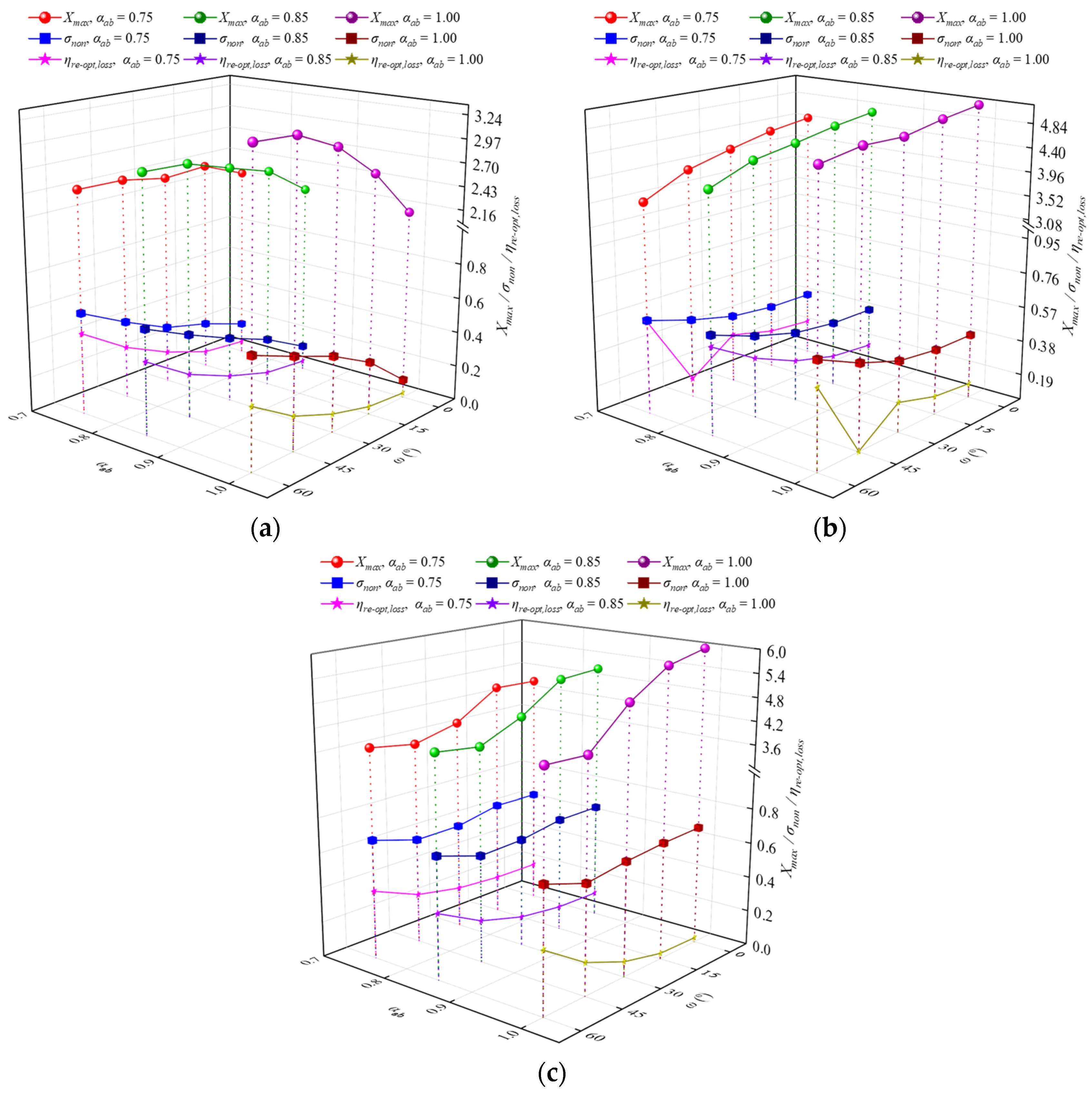
3.3. Effect of Receiver Internal Surface Absorptivity α_ab

After the specific case study, the parametric study was conducted to quantify the effects of α_ab on the optical performance of the system. The existence of δ causes the sunlight to obliquely enter the linear Fresnel lens and then move the focal line upwards, which leads to a decrease in the number of rays intercepted by the cavity absorber. Therefore, the α_ab has a great influence on the η_re-opt,loss. In addition, the reflection number of sunlight inside the cavity absorber is also greatly affected by the α_ab, which ultimately affects the σ_non, especially when the δ = 23.45°. In this section, for the receiver internal surfaces, three kinds of α_ab (0.75, 0.85, and 1.00) were considered, and the ω varying from 0° to 60° at the particular α_ab was numerically analyzed under the f = 650 mm (except for LACR) and ρ_r = 0.85. Figure 11a shows the effect of the α_ab on the optical performance of the FLSCS using LTCR.As shown in Figure 11a, the η_re-opt,loss increases with the decrease of α_ab, but its increasing trend gradually decreases with the increase of ω. For example, when the ω = 0° and 60°, the α_ab is 1.00, 0.85, and 0.75, the η_re-opt,loss is 2.47%, 4.68%, 6.32% and 35.56%, 41.73%, 46.53%, respectively. Referring to Figure 7a–c, as the ω increases, the distribution area of first intercepted sunlight gradually moves from two sides to one side, resulting in a gradual decrease in the number of secondary intercepted sunlight. Thus, the absorbed sunlight energy is increasingly dependent on the first interception, and the ratio of η_re-opt,loss is close to the ratio of α_ab when the ω = 60°. In other words, the cavity structure can be optimized to increase the number of incident sunlight reflections on the inner wall, thereby reducing the requirement for high α_ab. Moreover, as shown in Figure 11a, the X_max increases with the decrease of α_ab as the ω = 0°, while the X_max decreases with the decrease of α_ab for ω of 15–60°. In addition, the decreasing trend of X_max with the α_ab becomes more obvious for ω of 15–60°. This is because the incident sunlight is symmetrically distributed on both bottom sides of the cavity absorber when the ω = 0°. With the decreasing of α_ab, the number of the reflection of the sunlight on both bottom sides increases to form energy accumulation, increasing X_max. Referring to Figure 7a–c, as the ω increases, the distribution area of first intercepted sunlight gradually shifts to one side, part of the second reflected sunlight escapes, and the energy-concentration effect decreases. The X_max mainly depends on the energy flux distribution of the first intercepted sunlight. The greater the α_ab, the greater the X_max. The Δf decreases with the increase of ω, thus the energy flux density of first intercepted sunlight increases, resulting in a more noticeable difference in X_max with different α_ab. As shown in Figure 11a, the variation of σ_non is similar to that of the X_max. The σ_non increases with the decrease of α_ab as the ω = 0°, and the situation is the opposite for ω of 15–60°. It further shows that the X_max is far greater than the X_mean, and the σ_non mainly depends on the X_max. However, unlike the change of X_max, the decreasing trend of σ_non with the α_ab becomes gentle as ω increases in the range of 15–60°. This is because as the ω increases, the energy absorbed of first intercepted sunlight accounts for an increasing proportion of the total absorbed energy. In other words, the energy flux distribution mainly depends on the distribution of first intercepted sunlight. Therefore, the influence of α_ab on the σ_non is weakened.

As in the case of the LTCR, Figure 11b shows the effect of α_ab on the optical performance of the FLSCS using LACR. To avoid being affected by the occluded and escaped incident sunlight, the case of f = 675 mm is selected. As shown in Figure 11b, the η_re-opt,loss increases with the decrease of α_ab, but its increasing trend gradually decreases with the increase of ω. For example, when the ω = 0° and 60°, the α_ab is 1.00, 0.85, and 0.75, the η_re-opt,loss is 12.75%, 19.11%, 23.71% and 48.27%, 52.44%, 55.61%, respectively. Since the upward movement distance of focal line is 97.2 mm as δ = 23.45° and the f = 675 mm, referring to Figure 8a–c, as the ω increases, the distribution area of first intercepted sunlight gradually moves from the bottom to one side, resulting in a gradual increase in the number of secondary intercepted sunlight. Therefore, as the number of the reflection of sunlight in the cavity absorber increases, the effect of α_ab on the absorption of sunlight energy decreases gradually. Moreover, as shown in Figure 11b, the X_max decreases with the decrease of α_ab for ω of 0–60°. In addition, the decreasing trend of X_max with the α_ab is basically stable before ω = 45° but becomes obvious as ω increases in the range of 45–60°. Referring to Figure 8a–c, it can be inferred that the energy flux distribution mainly depends on the first intercepted sunlight, and with the increase of ω, there is an increase in the amount of escaped sunlight. Therefore, the influence of α_ab on the X_max is intensified, and the amount of escaped sunlight increases sharply for ω of 45–60°. When the ω = 60°, the α_ab is 1.00, 0.85 and 0.75, the X_max is 4.782, 4.034, 3.567, respectively, which is close to the ratio between the different α_ab. As shown in Figure 11b, the variation of σ_non is similar to that of the X_max. The σ_non decreases with the decrease of α_ab. Before ω = 45°, the variation of the σ_non with the α_ab can basically be ignored, but it becomes obvious as ω increases in the range of 45–60°. This is because the energy flux distribution mainly depends on the distribution of first intercepted sunlight, especially for ω of 0–45°. Therefore, the influence of α_ab on the σ_non is weakened. However, the amount of escaped sunlight increases sharply for ω of 45–60°, the distribution of second or more intercepted sunlight has an increased influence on the energy flux distribution. When the ω = 0° and 60°, the α_ab is 1.00, 0.85, and 0.75, the σ_non is 0.4065, 0.404, 0.4016 and 0.6205, 0.5864, 0.5636, respectively.

As in the case of the LTCR, Figure 11c shows the effect of α_ab on the optical performance of the FLSCS using LRCR as f = 650 mm. As shown in Figure 11c, the η_re-opt,loss increases with the decrease of α_ab, but its increasing trend gradually decreases with the increase of ω. For example, when the ω = 0° and 60°, the α_ab is 1.00, 0.85, and 0.75, the η_re-opt,loss is 2.47%, 12.86%, 20.99% and 36.08%, 37.75%, 39.06%, respectively. Referring to Figure 9a–c, as the ω increases, the distribution area of first intercepted sunlight gradually moves from the bottom to one side, resulting in a gradual increase in the number of secondary intercepted sunlight. Therefore, as the number of the reflection of sunlight in the cavity absorber increases, the effect of α_ab on the absorption of sunlight energy decreases gradually. Moreover, as shown in Figure 11c, the X_max decreases with the decrease of α_ab for ω of 0–60°. In addition, the decreasing trend of X_max with the α_ab decrease for ω of 0–60°. Referring to Figure 9a–c, it can be inferred that the energy flux distribution mainly depends on the first intercepted sunlight as ω = 0°, and with the increase of ω, the amount of secondary intercepted sunlight increases. Especially as ω = 60°, part of the incident sunlight fails to be intercepted and escapes. The influence of the secondary intercepted sunlight on the energy flux distribution gradually increases. Therefore, the influence of α_ab on the X_max decreases as the ω increases. When the ω = 60°, the α_ab is 1.00, 0.85 and 0.75, the X_max is 4.221, 3.986, 3.751, respectively. As shown in Figure 11c, the variation of σ_non is similar to that of the X_max. The σ_non decreases with the decrease of α_ab. It further shows that the X_max is far greater than the X_mean, and the σ_non mainly depends on the X_max. Noted that the decrease rate of σ_non presents continuous fluctuations for ω of 0–60°. However, the increase rate of the η_re-opt,loss and the decrease rate of the X_max is decreased for ω of 0–60°. In other words, the α_ab can affect the change rate of σ_non, but not the changing trend. When the ω = 0° and 60°, the α_ab is 1.00, 0.85, and 0.75, the σ_non is 0.682, 0.6663, 0.6558 and 0.7039, 0.6945, 0.6822, respectively.

3.4. Effect of End Reflection Plane Reflectivity ρ_r

The increase of the δ causes the light to enter the cavity absorber obliquely. The end loss can be effectively reduced by sliding the mirror element, and the sunlight reflected by the cavity absorber inner wall tends to propagate to one end. By setting the end reflection plane, the sunlight incident on the end can be reflected again so that it has a chance to be intercepted again by the cavity absorber to reduce the optical loss further. The end reflection plane itself has a role in the amount of sunlight reflected and lost. Thus, the effect of the end reflection plane in reducing the optical loss and its influence on the energy flux distribution is explained by studying end reflection planes with different ρ_r. In this section, for the end reflection planes, three kinds of ρ_r (0.75, 0.85 and 1.00) were considered, and the ω varying from 0° to 60° at the particular ρ_r was numerically analyzed. The f, α_ab and δ are 650 mm, 0.85, and 23.45°, respectively.

Figure 12a shows the effect of the ρ_r on the optical performance of the FLSCS using LTCR. It can be seen from Figure 12a that the η_re-opt,loss increases slightly as the ρ_r decreases when the ω is fixed. The average η_re-opt,loss for ρ_r = 1.00, 0.85, and 0.75 are 18.49%, 18.56%, and 18.60%, respectively, for ω of 0–60°. However, the average η_re-opt,loss is reduced by 0.46%, 0.39%, and 0.35%, respectively, compared to 18.95% if the end reflection plane is not installed. It can be inferred that the number of incident sunlight on the end reflection plane can be ignored compared to intercepted sunlight. The results prove that sliding the lens element can effectively solve the problem of end loss. In addition, as shown in Figure 12a, the X_max decreases with the decrease of ρ_r for ω of 0–60°. It is because part of the incident sunlight on the end reflection plane is reflected on the cavity absorber inner wall again, which causes the X_max to increase. However, the sunlight mentioned above energy decreases as the ρ_r decreases, decreasing the X_max. The average X_max for ρ_r = 1.00, 0.85, and 0.75 are 2.629, 2.586, and 2.565, respectively, for ω of 0–60°. The average X_max is increased by 3.91%, 2.21%, and 1.38%, respectively, compared to 2.531 if the end reflection plane is not installed. As shown in Figure 12a, the variation of σ_non with ρ_r is similar to that of the X_max. The σ_non decreases with the decrease of the ρ_r for ω of 0–60°. It is because the η_re-opt,loss of different ρ_r is almost constant for ω of 0–60°, resulting in a similar X_mean; thus, the σ_non depends on the X_max. The average σ_non for ρ_r = 1.00, 0.85, and 0.75 are 0.385, 0.372, and 0.366, respectively, for ω of 0–60°. The average σ_non is increased by 7.84%, 4.20%, and 2.52%, respectively, compared to 0.357 if the end reflection plane is not installed. This indicates that the optical loss can be slightly reduced by setting the end reflection plane. Still, compared with the cost of the end reflection plane and the increased non-uniformity of the energy flux distribution, the cost performance of setting the end reflection plane is low.

Figure 12b shows the effect of ρ_r on the optical performance of the FLSCS using LACR. It can be seen from Figure 12b that the η_re-opt,loss increases slightly as the ρ_r decreases when the ω is fixed. The average η_re-opt,loss at ρ_r of 1.00, 0.85, and 0.75 are 31.43%, 31.55%, and 31.64%, respectively for ω of 0–60°. It can be inferred that the number of sunlight incidents on the end reflection plane is negligible compared to the amount of intercepted sunlight by the cavity absorber. In other words, the end reflection plane can be replaced by insulating cotton, which reduces the cost of the system and reduces heat loss. In addition, as shown in Figure 12b, the X_max decreases with the decrease of ρ_r. The changing trend of X_max as f = 675 mm using LACR is similar to that of f = 650 mm using LTCR, and thus detailed analysis is omitted herein. The average X_max at ρ_r of 1.00, 0.85, and 0.75 are 4.755, 4.456 and 4.262, respectively for ω of 0–60°. As shown in Figure 12b, the variation of σ_non with ρ_r is similar to that of the X_max. The σ_non decreases with the decrease of the ρ_r for ω of 0–60°. It is because the η_re-opt,loss of different ρ_r is almost constant, resulting in a similar X_mean, and the σ_non depends on the X_max. The average σ_non at ρ_r of 1.00, 0.85, and 0.75 are 0.498, 0.465, and 0.441, respectively, for ω of 0–60°. This indicates that the effect of setting the end reflection plane on the optical efficiency of the system is negligible, and it will increase the hot spot effect on the cavity receiver inner wall.

Figure 12c shows the effect of ρ_r on the optical performance of the FLSCS using LRCR. It can be seen from Figure 12c that the η_re-opt,loss increases slightly as the ρ_r decreases when the ω is fixed. The average η_re-opt,loss at ρ_r of 1.00, 0.85, and 0.75 are 20.78%, 20.94%, and 21.04%, respectively for ω of 0–60°. It can be inferred that the number of sunlight incidents on the end reflection plane is negligible compared to the amount of intercepted sunlight by the cavity absorber. In addition, as shown in Figure 12c, the X_max decreases with the decrease of ρ_r. The average X_max at ρ_r of 1.00, 0.85, and 0.75 are 4.798, 4.459, and 4.244, respectively, for ω of 0–60°. The average X_max difference of different ρ_r is obvious, but the difference of average η_re-opt,loss of that is small. As shown in Figure 12c, the variation of σ_non with ρ_r is similar to that of the X_max. The σ_non decreases with the decrease of the ρ_r for ω of 0–60°. It is because the η_re-opt,loss of different ρ_r is almost constant, resulting in a similar X_mean, and the σ_non depends on the X_max. The average σ_non at ρ_r of 1.00, 0.85, and 0.75 are 0.676, 0.652, and 0.635, respectively, for ω of 0–60°. Therefore, introducing the end reflection plane will aggravate the non-uniformity of the energy flux distribution without significantly increasing the optical efficiency.

4. Conclusions

Optical performance comparison of different cavity receiver shapes in the FLSCS has been investigated. The analysis was conducted by studying the effects of sunlight incident angle θ, receiver position f, receiver internal surface absorptivity α_ab, and end reflection plane reflectivity ρ_r on the optical efficiency of system and flux uniformity of linear cavity receiver. The main results are summarized as follows:

(1)

The increases of δ in the range of 0–8° have a weak effect on the η_re-opt,loss. The η_re-opt,loss are 2.25%, 2.72%, 12.69% and 2.62%, 3.26%, 12.85%, respectively when the ω is 0°, 30°, 60° for δ = 0° and 8° for LTCR. The increase of ω can affect the number of secondary intercepted sunlight. The η_re-opt,loss are 14.99%, 14.72%, and 2.61%, respectively when the ω is 0°, 15°, 60° when the δ = 0° for LACR.

(2)

The increase of f can affect the number of first intercepted sunlight. When the f is 600, 625, 650, 675, 700 mm and the ω = 60°, the η_re-opt,loss are 16.72%, 5.48%, 2.47%, 3.17%, 14.43%, respectively, for LRCR. The increase of α_ab can affect the reflection number of sunlight. When the ω = 0° and 60°, the α_ab is 1.00, 0.85, and 0.75, the η_re-opt,loss is 2.47%, 12.86%, 20.99% and 36.08%, 37.75%, 39.06%, respectively for LRCR. The increase of ρ_r has little effect on the η_re-opt,loss. When the ω = 0° and 60°, the α_ab is 1.00, 0.85, and 0.75, the η_re-opt,loss is 12.75%, 19.11%, 23.71% and 48.27%, 52.44%, 55.61%, respectively, for LACR.

(3)

The X_max mainly depends on the energy flux distribution of first intercepted sunlight on the cavity absorber inner wall. The increase of δ can affect the Δf. The smaller the Δf, the greater the X_max, and vice versa. When the δ is 0°, 8°, 16°, and 23.45° and the ω = 60°, the X_max are 6.461, 5.950, 4.428, and 2.773, respectively, for LTCR. The increase of ω can affect the X_max due to the Δf change with the increase of ω. The X_max are 5.896, 7.140, and 6.969, respectively, when the ω is 0°, 45°, and 60° when the δ = 0° for LACR.

(4)

The increase of f can affect the X_max significantly. When the f is 600, 625, 650, 675, and 700 mm and the ω = 60°, the X_max are 5.832, 6.949, 6.969, 6.509, and 5.699, respectively, for LRCR. The increase of α_ab can affect the X_max significantly as the reflection number of sunlight is small. When the ω = 0°, the α_ab is 1.00, 0.85, and 0.75, the X_max is 5.999, 5.108, 4.511, respectively for LRCR. The increase of ρ_r has little effect on the X_max. For LACR, the average X_max at ρ_r of 1.00, 0.85, and 0.75 are 4.755, 4.456, and 4.262, respectively, for ω of 0–60°.

(5)

The changing trend of σ_non is basically consistent with that of the X_max. The increase of δ can affect the σ_non due to the Δf change with the increase of δ. When the δ is 0°, 8°, 16°, and 23.45° and the ω = 60°, the σ_non are 0.737, 0.715, 0.662, and 0.591, respectively, for LTCR. The increase of ω can affect the σ_non due to the Δf change with the increase of ω. The σ_non are 0.494, 0.536, and 0.510, respectively, when the ω is 0°, 45°, and 60° when the δ = 0° for LACR. The increase of f can affect the σ_non significantly. When the f is 600, 625, 650, 675, and 700 mm and the ω = 0°, the σ_non are 0.832, 0.828, 0.801, 0.747, and 0.671 respectively for LRCR.

(6)

The increase of α_ab and ρ_r affect the σ_non but not obviously. When the ω = 0° and 60°, the α_ab is 1.00, 0.85, and 0.75, the σ_non is 0.682, 0.6663, 0.6558 and 0.7039, 0.6945, 0.6822, respectively for LRCR. For LACR, the average σ_non at ρ_r of 1.00, 0.85, 0.75 are 0.498, 0.465, 0.441, respectively, for ω of 0–60°.

Finally, through comparison with cavity receiver such as LFR and PTC, it is found that LTCR is suitable for FLSCS because of its better optical performance. Since the FLSCS is installed obliquely north–south, the I_d increases significantly for the Tropic of Cancer and its north when the δ is +23.45° (the summer solstice of the Chinese calendar). When the δ is between 8° and 23.45°, the focal line moves up obviously with the increase of δ, which leads to the decrease of the system’s optical efficiency and becomes more obvious with the increasing of the δ. To obtain the maximum annual total solar radiation for the solar system, these factors need to be considered in the future to match the optical performance of the FLSCS with the annual variation of I_d.