Research on Sustainable Development of the Regional Construction Industry Based on Entropy Theory

Abstract

Human beings are now facing the increasingly urgent problem of global ecological environment pollution. To verify the scientific nature of environmental governance by governments of various countries, researchers need to provide a scientific basis and practical support for governments to adjust and formulate new policies and regulatory measures at any time through data analysis. This paper applies visual literature, aggregate analysis, engineering data programming, advanced mathematical science algorithms, and innovation entropy theory, and through this study obtains sustainable impact data from eight Chinese provinces in the 21st century, including environmental, economic, and social impacts. The results show that China’s sustainable data should grow from 2021 to about 2044. After 2045, it will be stable, and there will be negative growth in a short period. The overall life cycle assessment (LCA) and social impact assessment (SIA) continue to remain in the positive range. There will be no negative growth in aggregate data and zero or negative emissions before 2108. The final research data are accurately presented in the form of annual emissions, which provide a scientific and theoretical basis for the government to formulate medium- and long-term ecological regulations and plans.

1. Introduction

The Intergovernmental Panel on Climate Change (IPCC) Special Report on Emergency Scenarios predicted an increase of 45% in the global emissions of greenhouse gases from 2000 to the 2030 year (carbon dioxide-eq (CO₂-eq)), with over USD 20 trillion investment in energy infrastructure. It also predicted that fossil fuels might maintain their dominance [1]. By 2050, the CO₂-eq emissions will be steadily reduced to 445 ppm, even to zero by 2070, and then less than zero (harmful emissions) [2]. The Integrated Assessment Model for the Global Climate Economy has shown that an additional 430~740 Gt CO₂ will be removed globally by 2100 [3]. There is a large consumption of energy and fossil materials in the construction industry, which plays a vital role in causing global emissions of greenhouse gas [4]. As a result, countries worldwide have established many measures, including decarburization, low carbon, carbon neutrality, carbon capture, storage, etc. [5].

As the world’s largest emitter (about 28% of all world emissions [6]), and with emissions in the construction industry being responsible for 31.9% of the total [7], at the 75th Session of the United Nations General Assembly in 2019, China announced that it will reach its peak by 2030 and reach carbon neutrality by 2060 [8]. Duan et al. [9] have developed a multi-model study of China, showing that achieving the target would require reductions in carbon emissions and energy consumption of more than 90% and 39% in 2050 and a reduction in fossil fuels by more than 73%, as well as a fall in demand for coal to near zero (compared with 2009).

The United States is the second-largest emitter globally, accounting for 15% of the global total, with emissions in the construction industry responsible for 36% of the total. It aims to cut greenhouse gas emissions by 80% by 2050 (compared with 2005) through the following three steps: transition to a low-carbon energy system (for example, wind energy, water energy, etc.), carbon sequestration through a forest, soil and removal technology, and a reduction in the production of fossil fuels [10]. By assessing the emissions reduction potential of the United States construction industry in 2050 through an electrification and high renewable energy permeability combination technique, Jared et al. have predicted a 72–78% reduction, slightly below this goal [11].

There are different standards of administrative division in various countries, including provinces, states, commonwealths, regions, etc. It shows significant differences in economic growth, technological progress, population density, industrial structure, and resource endowment in different regions, which cause significant differences in sustainable impacts. Sustainable development (SD) provides a perfect solution to modern urban ecology, social aspirations, and economic issues [12,13]. By analyzing the complex interactions of different systems, sustainability provides robustness for a sustainable society with technological advances, to address urban development [14].

In the 12th Five-Year Plan, the 13th Five-Year Plan, and the 14th Five-Year Plan, the State Council of the People’s Republic of China proposed different economic targets and cut emissions to determine the provincial quota allocation standard. The quota is directly associated with per capita GDP (per capita gross domestic product), per capita income and family wealth, etc. [15], which has been the responsibility and principle for determining fair, familiar, but the differentiated capacity to cope with climate change [16].

An analysis of the research papers shows that reaching the carbon emissions targets in the construction industry in different countries and regions plays a crucial role in the solutions for global ecological pollution and serves as a basis for realizing the climate targets of The Paris Agreement by the middle of this century (2050) [17].

The main objectives of this paper are as follows:

• The study analyzes the local primary data released by the government from 2000 to 2020 through the established statistical regression mathematical model and to determine the validity of discrete data through the Fourier sine transform, deleting the invalid data, establishing a vector matrix, and making the least-square regular fitting for valid data. The paper also aims to determine the final effective curve as a mean entropy model.
• To establish the GDP mathematical analysis model according to the overall goal set by the state (Section 4.6), to analyze the practical value of sustainability in eight provinces from 2020 to 2100 (IPCC provides that a Three Pillars study will be made) [18].
• To determine the rationality and validity of overall national targets based on data from objective 2 and to provide a scientific basis for similar government policies in the global construction industry.
• To analyze the potential of each province’s sustainable control and emission reduction and evaluate the changes in growth rate through an innovative model.

This study is innovative in the following respects:

• Exploring and scientifically demonstrating the accuracy and feasibility of China’s carbon emission targets for 2030 and 2060 through a 100-year practical assessment of the sustainability of the construction industry in the top eight economic provinces.
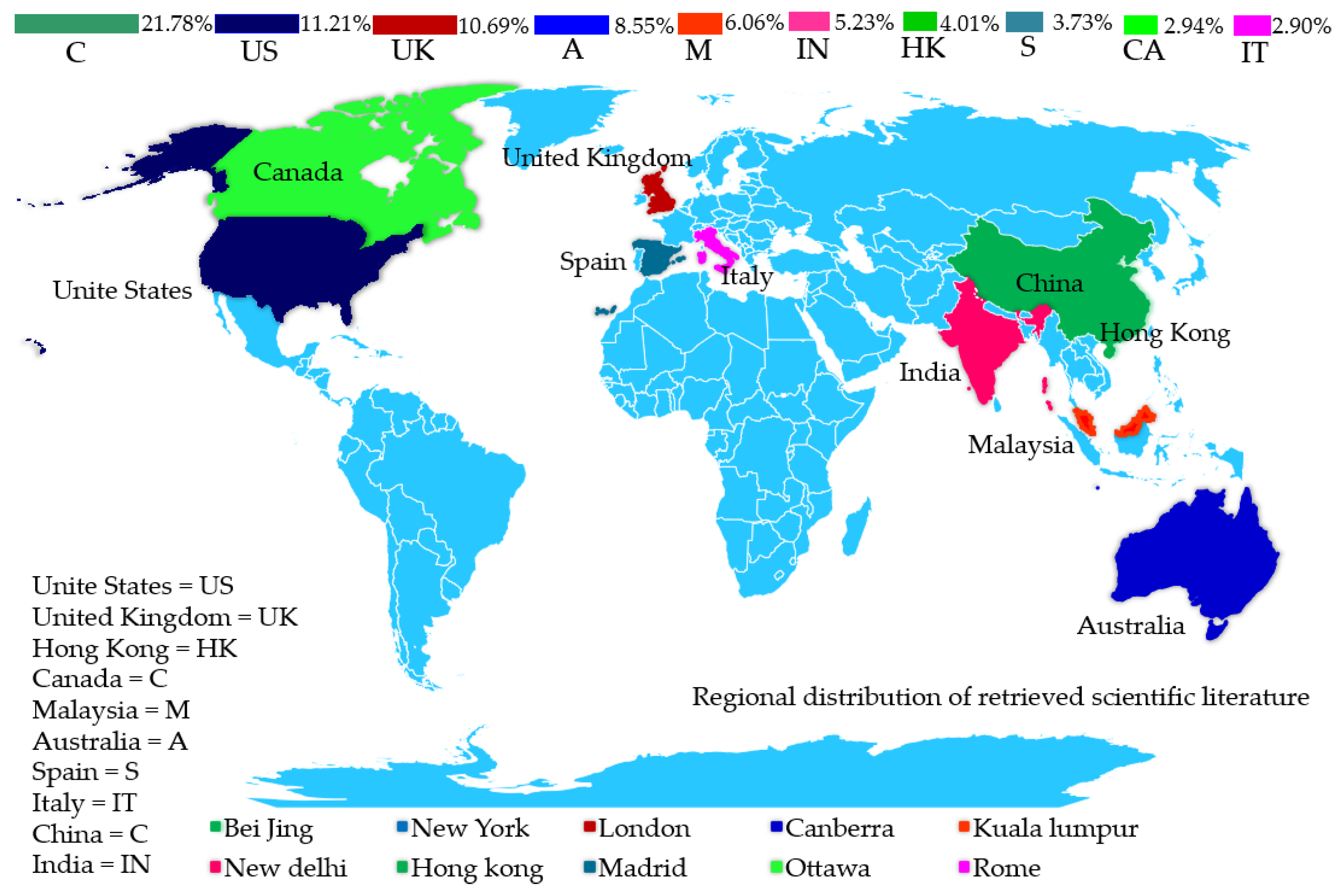
• Searching the relevant literature with no similar literature in this field (see Section 2 for details).
• Developing a scientific algorithm and theoretical model for global construction industry development assessment through interdisciplinary fusion research, from the given data to computing future impact data and checking official statistics’ scientific accuracy and feasibility.
• Establishing an entropy weight model to improve the determination of the influence and importance of impact assessment data.

2. Literature Review

To determine the latest research on related subjects, Cite Space software was used to develop a visual bibliometrics coupling analysis [19]. The discussion was made from six dimensions by searching 33,179 articles in total, carrying out cluster analysis based on keywords, and selecting the top ten countries with publications listed below (Figure 1). $Q$ > 0.49 in cluster coupling analysis indicates a significantly accurate clustering structure, and $S$ > 0.76 shows that the cluster data analysis was made reasonably, with accurate results and high reliability (

Table 1. Cluster metrology analysis parameters.

Keyword	Negative Emissions Articles
	China	United States	United Kingdom	Australia	Malaysia	Scope
Number	2604	1340	1278	1023	725	⁄
Time span	1995–2022	1993–2022	1993–2022	1995–2022	1997–2021	⁄
Number of nodes	846	790	795	693	519	⁄
Number of connections	3372	3470	3445	2774	2004	⁄
Large co-citation	805	752	739	646	481	⁄
Modularity: $Q$	0.557,1	0.548,3	0.553,7	0.564,5	0.613,7	0.3 < $Q$
Silhouette: $S$	0.756,7	0.789,1	0.789,9	0.793,1	0.816,1	0.5 < $S$ < 1
Harmonic mean: $Q$, $S$	0.641,7	0.647	0.651	0.659,6	0.700,6	$Q$,$S$ = 0.5
Keyword	Negative Emissions Articles
	India	Hong Kong	Spain	Canada	Italy	Scope
Number	626	480	446	352	347	⁄
Time span	1995–2021	2000–2022	2004–2021	1996–2021	1997–2021	⁄
Number of nodes	571	614	496	584	515	⁄
Number of connections	2132	2579	2042	2242	2042	⁄
Large co-citation	518	552	460	534	480	⁄
Modularity: $Q$	0.610,1	0.583,1	0.590,2	0.636	0.636,3	$0.3< \mathrm{Q}$
Silhouette: $S$	0.827,6	0.812	0.826,1	0.840,5	0.839,9	$0.5 < \mathrm{S}$< 1
Harmonic mean: $Q$, $S$	0.702,4	0.678,8	0.688,5	0.724,1	0.724	$\mathrm{Q}$,$S$ = 0.5

).

Keywords for the literature search included “construction industry”, “SD”, and “article (selecting “article” in the literature restricts the retrieval content and has a more paradigmatic format. The article constructs the core system of scientific research [8])”, with 11,958 papers being searched.

To further improve the quality of visual clustering analysis, the research scope was extended by selecting the top 10 countries for cluster coupling analysis (Table 1). The cluster module $Q$> 0.5 showed a significant clustering structure, and the clustering average contour $S$> 0.75 indicated accurate clustering results, while a $Q$ and $S$ of about 0.5 shows that the structure was robust.

The top three in the target evaluation of research modules in ten countries are 21.78% (China), >11.21% (United States), and >10.69% (United Kingdom). The literature contribution in this field shows a quadratic parabola path in the mass and is estimated to increase continuously in the future. The interpolation approximation fitting analysis was made on the track of published literature in each country to develop a 3D (three-dimensional) curve diagram of a thin plate spline to represent the research focuses of the literature (Figure 1). In the past 30 years, the United States, China, and Hong Kong have shown negative values in the middle stage and then stepped into a growth stage, while Canada and the United Kingdom have presented positive values in the middle stage and then started to decrease. Spain and Australia have been in the stage of reduction and continue to decrease, while Italy, India, and Malaysia have been in the stable development stage. Malaysia is showing a short-term decrease in short duration.

The top 10 most-cited keywords in clustering have been selected to show the main research directions and scopes of ten countries in this field. China places importance on green buildings and carbon emissions. At the same time, the United States emphasizes carbon emissions from building materials and related fields, and Britain stresses building structures and clean energy. Australia emphasizes building materials and building information management. The ten countries have in common that the research is specific and specialized. SD is only seen in India and Canada, ranking seventh and tenth, respectively. Furthermore, there has been no literature on the construction industry’s impact on society for a long time (Figure 2).

Through the above literature survey and research, it can be found that there is a significant gap in the contribution of countries around the world to sustainable development. At the same time, sustainable development research in the construction industry is gradually declining. Although the research scope is expanding, there are areas for improvement in the validity and practicality of the research field. In particular, there are gaps and defects in the in-depth analysis and comprehensive research of SIA in the construction industry, as well as the scientific speculation and assessment of future sustainable development. This field needs to be supplemented and improved.

3. Methodology

Bridge LCC and LCA are commonly used research methods to reduce material consumption and cost. Evaluation and analysis are carried out by quantifying the two and the delineated system boundary [20]. Using materials in the construction industry promotes the excessive consumption of global natural resources (fossil energy) and causes environmental problems such as global warming and resource shortages. The consumption of raw materials accounts for 40% of the total energy and produces 50% of carbon emissions [21]. Thus, research on sustainability in the construction industry refers to an effective solution to service programs, from planning and design to analyzing the system’s removal upon service expiration (birth to death). As defined in the Rio Declaration on Environment and Development, assessing SD in the construction industry covers three fundamental pillars: environmental, economic, and social impacts [22].

The theoretic framework and system for this paper were established according to ISO14040(2006), The Paris Agreement (IPC2015,2017), and the 24th Conference of the Parties to the United (UNFCCC, COP24), which was held in Kartowitz, Poland, in 2018 (Figure 3) [23,24,25].

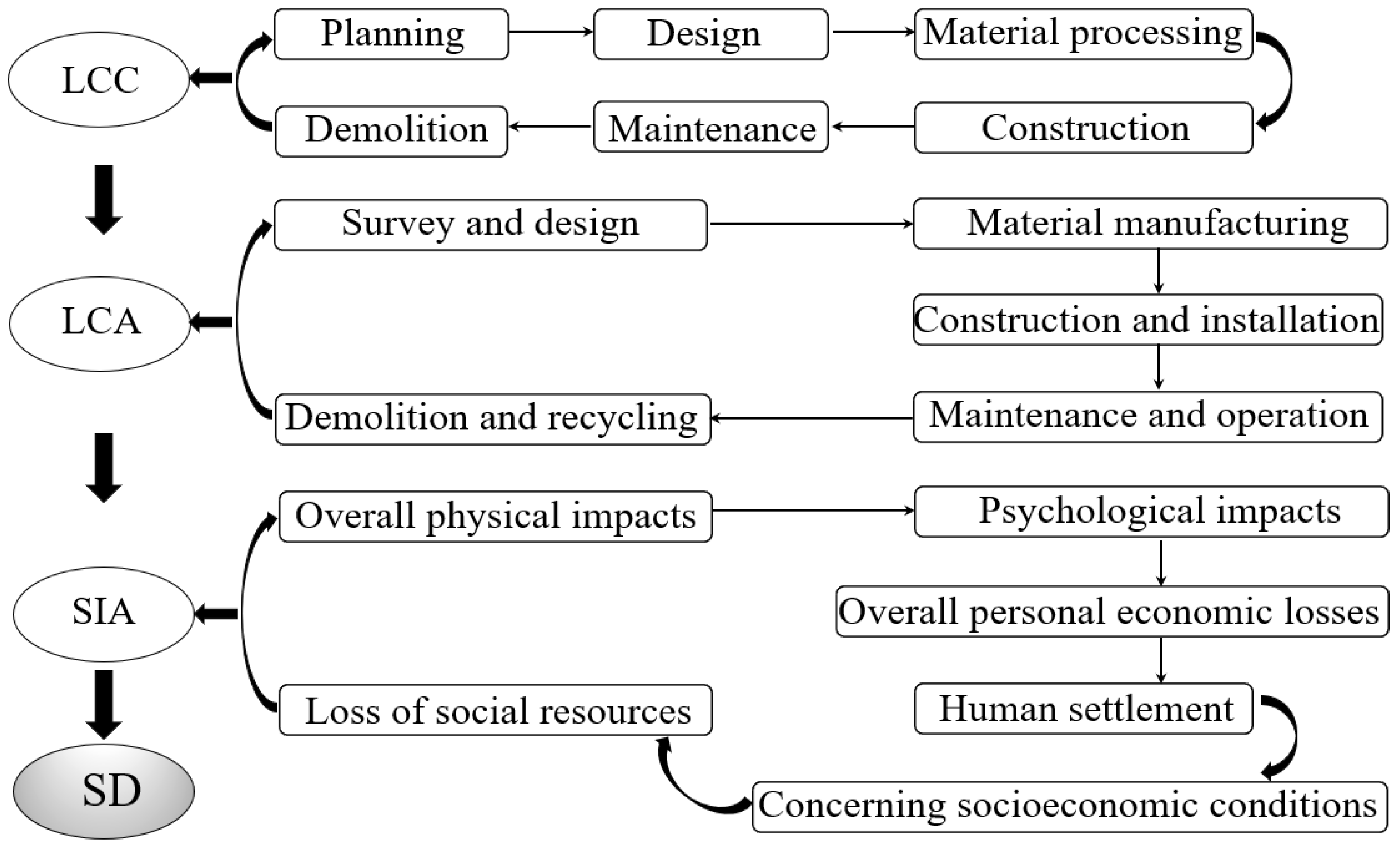
3.1. Models of LCA, LCC, and SIA

ISO14040 (2006) defined LCA as the “Collection and Assessment of Input, Output and Potential Environmental Impact over the Whole Life Cycle of Product System.” Zhou et al. [22] studied the sustainability of six bridges in different regions of China and established a complete assessment model as a reference. Since bridge construction significantly influenced the regional construction industry, five stages of bridge construction were studied (Figure 3). OpenLCA 1.10.1 analysis software was chosen for the life cycle assessment, with Ecoinvent, Bedec, China Statistical Yearbook, and many published papers as the database [26].

The LCA framework was defined with ten key influences: human toxicity, ozone layer depletion (ODP), abiotic depletion, eutrophication, acidification, freshwater aquatic ecotax, global warming (GWP100a), marine aquatic ecotoxicity, photochemical oxidation, and terrestrial ecotoxicity, by the ISO standard. The midpoint method was used for stage analysis in LCA, while the endpoint method was used for comprehensive analysis [27]. It is essential to select the assessment units correctly in LCA research; thus, Kg was used as the assessment unit since the bridge structure comprised sections of multiple material combinations [28].

Bridges are designed for a 100-year lifespan in China. The comprehensive LCC evaluation is highly complicated, with low accuracy, and no comprehensive and accurate computing model has yet been found [29,30,31]. It is not plausible that the structural service life parameters were ignored in the maintenance stage for a long-span cable-stayed bridge. Otherwise, it reduces the robustness of the study. Specifications for Highway Cable-stayed Bridge JTG/T3365-01, General code for design of highway bridges and culverts JTGD60-2015, and Highway Engineering Budgetary Estimate Quota JTG3831-2018 have specified the service life cycle of the members, which shall be calculated as per the standard data in the specifications [28].

$$C_{\mathrm{Total}} =(C_{\mathrm{Design}}+C_{\mathrm{Material}}+C_{\mathrm{Construction}}+C_{\mathrm{Maintenance}}+C_{\mathrm{Demolition}})\times (1\pm r{)}^{-1}$$

(1)

where $C_{\mathrm{Total}}$ is the total cost of the bridge (USD is the United States dollars). $C_{\mathrm{Design}}$ is the cost of planning and design (USD). $C_{\mathrm{Material}}$ is the cost of raw material (USD).$C_{\mathrm{Construction}}$ is the cost of construction (USD). $C_{\mathrm{Maintenance}}$ is the cost of maintenance (USD).$C_{\mathrm{Demolition}}$ is the cost of removal and cleaning (USD)$,\mathrm{and}r$ is the discount rate (%).

SIA uses OpenLCA 1.10.3 as analysis software and the Product Social Impact Life Cycle Assessment (PSILCA). LCA analysis data may be correlated, improving the research’s systematic Ness and consistency. There are 54 qualitative and quantitative indexes from 18 categories. In the PSILCA database, 18 have been used for social impact assessment in the research [32].

3.2. Theory Model of Scientific Algorithm

Lagrange polynomial is a standard formula for polynomial interpolation calculation in theoretical analysis and numerical applications to solve multidimensional, variable numerical problems [33]. The multidimensional polynomial function ($R^2$, SSE) was built from the data acquired. Moreover, SD data were fitted to obtain estimated data by approximating multidimensional functions with high precision by polynomial interpolation.

The variables $x$ and $y$ are transformed into [34]:

$$L_k\left(x_m,y_n\right)=\psi \left(f\left(x_{m-1},y_{n-1}\right)\right)+{{\displaystyle \int }}_a^x{{\displaystyle \int }}_a^{y}k\left(x_{m-1},y_{n-1};s,t;f\left(s,t\right)\right)dsdt+{\displaystyle \sum }_{\mu =0}^{y_{\mu }}{\displaystyle \sum }_{v=0}^{y_v}{x}_{\mu v}\left(x,y\right)\frac{{\partial }^{y}f\left(x,y\right)}{\partial x^{\mu }\partial y^v},\left(x_{m-1},y_{n-1}\right)\in D$$

(2)

where $L_k\left(x_m,y_n\right)$ is the $k^{th}$ function in two dimensions after transformation, $\mu$ are 0,1,$\cdots ,y_{\mu }$. $v$ are 0,1,$\cdots$,$y_v$. $y_{\mu }$ > 0 & $y_v$ > 0. $x_{\mu v}\left(x,y\right)$, $\psi \left(f\left(x_{m-1},y_{n-1}\right)\right)$, $k\left(x,y;s,t;f\left(s,t\right)\right)$ is the continuous function in each interval.

Set the interpolated values into a group matrix:

$${\displaystyle \sum }_{i=1}^{i=+\infty }{L}_k^i\left(x_m,y_n\right)=\left[\begin{array}{cccc}{L}_1\left(x_1,y_1\right)& L_1\left(x_1,y_2\right)& \cdots \cdots & L_1\left(x_1,y_n\right)\\ L_2\left(x_2,y_1\right)& L_2\left(x_2,y_2\right)& \cdots \cdots & L_2\left(x_1,y_n\right)\\ ⋮& ⋮& ⋮& ⋮\\ ⋮& ⋮& ⋮& ⋮\\ L_k\left(x_m,y_1\right)& L_k\left(x_m,y_2\right)& \cdots \cdots & L_k\left(x_m,y_n\right)\end{array}\right]$$

(3)

$\mathrm{where}{{\displaystyle \sum }}_{i=1}^{i=+\infty }{L}_k^i\left(x_m,y_n\right)$ are $k^{th}$ group of influence numerical matrix, and $k,m,n$ refer to effective influence variables.

Equation (3) refers to a numerical solution for a multidimensional, discrete interpolation matrix, which provides the original analysis data with fast convergence speed, high accuracy, and stability after double or multiple integral transformations. It solves discrete data error estimation and convergence analysis [35].

4. Results and Discussion

The accurate selection of research cases is the actual evaluation and verification of the method established in this paper. The ultimate goal of this study is to obtain robust data through optimal causal inference and quantitative regression analysis. Its core problem is to choose the best-case framework for solving research questions [36]. The bridges in the top eight provinces in China’s GDP were used as case studies (the research selection criteria are the four criteria listed in

Table 2. Relevant data from eight provinces (2019; tonnes; SCE, standard coal energy).

Province	Population (Ten Thousands)	GDP (100 million USD)	Consumption of Energy (10,000 t of SCE)	Gross Output Value of Construction Enterprises (100 million USD)
Guang Dong	12,601.251	16,059.99	31,122.99	2411.79
Jiang Su	8474.802	14,893.93	32,525.97	4799.92
Shan Dong	10,152.745	10,603.48	40,810.54	2167.31
Zhe Jiang	6456.759	9368.68	22,392.77	1874.04
He Nan	9936.552	7974.40	22,300.00	1841.70
Si Chuan	8367.487	7046.674	16,382.20	2550.86
Fu Jian	4154.009	6365.93	13,718.31	1908.80
Hu Bei	5775.256	6058.19	15,019.74	2461.99
China’s total	141,177.872	147,314.80	487,000.00	36,023.86
Ratio	46.69%	53.20%	39.89%	55.56%

, and the data ranking of the eight provinces ranks among the top eight in China), and the data are shown in Table 2. Furthermore, the data cited in this research were all from the China Statistical Yearbook, released by the National Bureau of Statistics of China on their official website, with recognition, accuracy, and decision making representing the latest industry authority in China [37].

Analyses of the fitting curve of data in the eight provinces in 2019 (goodness of fit $R^2$= 1) have shown that the top eight provinces in GDP have developed consistently with China. Studying the 100-year sustainable impacts in the regions plays a vital role in the deep analysis of national macro impacts and explicitly reflects the conditions and climate characteristics of the energy fields [38].

Analysis has been made on the data of population, reg GDP, consumption of energy, and the gross output value of construction enterprises closely associated with SD in eight provinces from 2010 to 2020 to improve the comprehensiveness of the research [22], as shown in Figure 4 and Figure 5.

The linear fitting analysis of the influencing factors shows that economic structure change, energy intensity efficiency, and total construction output value reflect the flexible changes in mechanisms in China’s short- and long-term development. This shows the significance of dynamic correlation analysis on data in SD analysis in China when building an integrated assessment model of the characteristic features of the gross domestic product. Figure 5a–h show the goodness of fit of variables 0.9988 > $R^2$ > 0.6431 and a mean value of 0.9575, which fully demonstrates the accuracy of the fitting.

The computational procedure by Wolfram Mathematics has been compiled herein to make a comparative analysis of reg GDP (Figure 5i), which shows that the changes in five provinces are in good agreement with the national trend, presenting low speed. The other three provinces show faster growth, and their curves invert the national linearity.

Bridges are one of the main connectors in infrastructure networks, showing the most significant impact on the road traffic function. The environmental, economic, and social diversity and complexity ratings are the benchmarks to measure the SD of the construction industry [39]. Eight cable-stayed bridges were selected in the case (

Table 3. The main data of the eight-bridges design technical standards.

Provinces		Guang Dong	Jiang Su	Shan Dong	Zhe Jiang
Design name		Zhanjiang Hai Wan Bridge (ZWGB)	Xia Jia, He Bridge (XJHB)	Lou Lan Bridge (LLB)	Rui ’An Bridge (RAB)
Bridge type	Main bridge	60 + 120 + 480 + 120 + 60 m (Double pylon)	68.358m (Single pylon)	20 + 232 + 32 + 20 m (Single pylon)	240 + 170 + 60 m (Single pylon)
	Approach bridge	9×50 + 9×50; 8×50 + 8×50m	4×20 + 3×20m	/	33×30 + 5×50 m; 8×30 + 20×50 m
Bridge deck width		28.5; 25.5 m	30 m	7 m	36.8 m (Main beam);33 m
Stay Cable		Φj 15.24 high-strength steel wires; ultimate tensile strength of 1860 Mpa.	163Ø7 parallel steel wires, ultimate tensile strength of 1670 Mpa.	OVM200 grade steel stranded cable, the standard strength is 1860 Mpa	Adopt the diameter Ø7 polyethylene parallel steel wire rope
Bridge structure	Main bridge	The main bridge is a pre-stressed concrete box girder with a beam height of 3 m. The thickness of the top plate and the inner web of the section is 0.25 m, and the thickness of the bottom plate is 0.22 m.	Pre-stressed concrete box girder: The cross-bridge of the box girder adopts a single-box double-chamber section, and the beam height is 2.0 m. The thickness of the top plate of the box girder is 25 cm; the thickness of the bottom plate is 20 cm; the thickness of the side web is 60 cm.	The main beam is 1.0 m high, the side web is 80 cm thick, the middle web is 30 cm thick, the top plate is 20 cm thick, and the bottom plate is 20 cm thick.	The main beam section is 3.2 m high; the top plate is 0.28 m thick, the bottom plate is 0.4 m thick, and the web is 0.4 m thick.
	Approach bridge	The beam is a continuous box girder with a beam height of 2.6 m, a top plate width of 12.74 m, and a bottom plate width of 5.56 m; the top plate is 25 cm thick; the bottom plate is 25 cm thick, and the web thickness is 40 cm.	20 m concrete simple beam; Each hole has 28 pre-stressed concrete hollow slab beams with a beam height of 0.9 m.	/	30 m box girder is 1.8 m high; the top plate thickness is 0.25 m, the bottom plate thickness is 0.2 m; web thickness is 0.6 m; 50 m box girder is 2.8 m high, the top plate thickness is 0.25 m, the bottom plate thickness is 0.5 m, web thickness is 0.75–0.50 m.
Substructure		Abutment; Pier column; Solid pier; Pier column	Abutment; Pier column; Solid pier; Pier column	Solid pier; Abutment; Pile foundation	Solid pier; Abutment; Pile foundation
Construction period		30/07/2003–30/12/2006	10/07/2017–29/06/2019	21/05/2011–11/06/2012	30/06/2003–13/01/2009
Estimated cost		0.174 billion USD	5.617 million USD	/	/
Bridge function		Cross-sea highway bridge	Cross-river highway bridge	Highway bridge	Highway bridge across the Yangtze River
Provinces		He Nan	Si Chuan	Fu Jian	Hu Bei
Design name		Xiantao Han River Highway Bridge(XTHB)	Peng Xi, He Bridge(PXHB)	Lu Yang Sea-crossing Bridge (LSCB)	E-Huang Yangtze River Bridge (EHYB)
Bridge type	Main bridge	2 × 50 + 50 + 82 + 180 + 2 × 50 m (Single pylon)	158 + 316 + 158 m (Double pylon)	80 + 103 + 380 + 103 + 80 m (Double pylon)	55 + 200 + 480 + 200 + 55 m (Double pylon)
	Approach bridge	14×30 m;18×30 m	8×40 m; 40 m	80 + 140 + 140 + 80 m; 44×80 m; 290×70 m; 88×35 m	300 + 1380 m
Bridge deck width		23 m/1472 m	24.5 m/1001 m	28 m/28136 m	24.5 m/2670 m
Stay Cable		Use diameter φj15.24PE galvanized steel strand	Ø7 Galvanized high-strength steel wire, standard strength 1670 Mpa.	The stay cable is cold cast anchored parallel steel wire lashing cable, the maximum specification is 211-φ7.	The stay cable adoptsΦ7 low-relaxation high-strength parallel galvanized steel wire, the standard strength of the steel wire is 1670 Mpa
Bridge structure	Main bridge	The roof thickness of the main beam is 0.30 m, and the beam height is 1.9 m	The beam height is 3.0 m, the roof thickness is 0.25m and the web thickness is 0.25–0.35 m.	The main girder is a single-box three-chamber box girder with a girder height of 3.8 m, a bridge deck width of 28.0 m, and a precast standard section length of 3.0 m.	The beam height is 2.4–4.9 m, and the bridge deck is 32 cm thick. The standard spacing of beams is 8 m.
	Approach bridge	30 m simply supported T-beam, 10 beams are arranged in the full width of the bridge and the beam distance is 2.30 m	Pre-stressed concrete main beam.	The main girder is a single-box single-chamber box girder; the girder height ranges from 8.0 to 4.0 m, the standard section length is 4.0~5.0 m, and the top section beam weight is 170 t.	The deputy main bridge is 300 m long, and the approach bridge is 1380 m long.
Substructure		Solid pier; Abutment; Pile foundation	Solid pier; Abutment; Pile foundation	Solid pier; Abutment; Pile foundation	Solid pier; Abutment; Pile foundation
Construction period		30/06/2003–13/01/2010	20/03/2004–26/05/2008	01/07/2002–30/06/2005	01/07/2002–30/06/2006
Estimated cost		0.435 billion USD	/	/	1.032 billion USD
Bridge function		Highway bridge across the Yangtze River	Cross-river highway bridge	Cross-sea highway bridge	Highway bridge across the Yangtze River

).

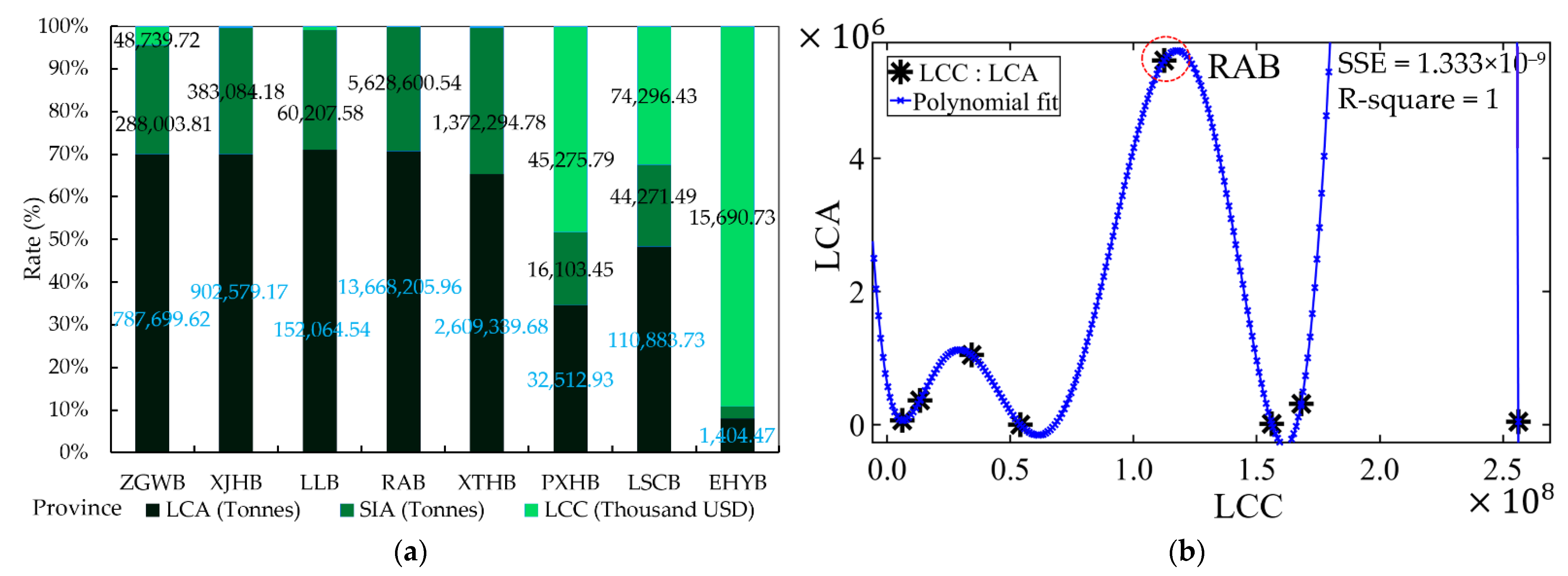
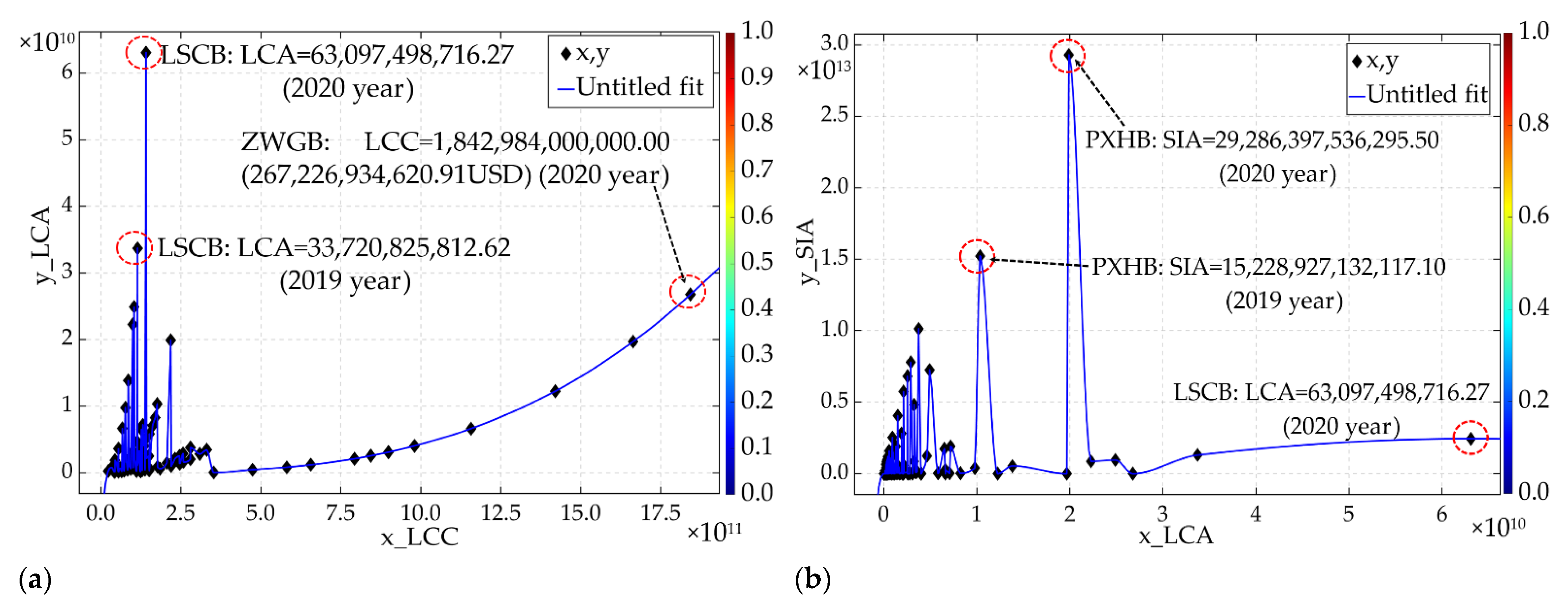
4.1. Analysis of LCC

The cases in this research are all Class I Expressway bridges in China. The survey and design cost shall be implemented by the document ((2002) No. 10) issued by the Ministry of Construction of China in 2001. In 2015, the National Development and Reform Commission of China ((2015) No. 299) announced that it was to fully lift the moratorium on engineering surveying and design fees and apply the market-modulated price [40]. However, the original document No. 10 still applies herein.

A road construction survey fee = the base price of engineering survey × physical workload × additional adjustment coefficient. XJHB, LLB, and PXHB are expressway bridges, of which the base price is 9787.29 USD/central line-km, and the additional adjustment coefficient is 2–3. ZJWB, RAB, XTHB, LSCB, and EHYB are Class I road bridges, of which the base price is 15,369.67 USD/central line-km, and the additional adjustment coefficient is the same as that of an Expressway [41] (

Table 4. The total cost of the project in the construction stage (USD).

Number	Name	Calculation Method	ZGWB	XJHB	LLB	RAB
1	Labor Costs	Quota × working days	234,732.35	55,869.94	36,450.74	258,875.16
2	Direct Costs	Labor + Material + Mechanical	4,849,841.56	354,264.47	129,557.64	3,177,976.78
3	Equipment Purchase Costs	1.899%×1	92,098.49	6727.48	2460.30	60,349.78
4	Measures Costs	4.381%×1	10,283.62	2447.66	1596.91	11,341.32
5	Enterprise management fees	4.143%×2	200,928.94	14,677.18	5367.57	131,663.58
6	Regulation fees	30.65%×1	71,945.47	17,124.14	11,172.15	79,345.24
7	Profits	7.42%×5	14,908.93	1089.05	398.27	9769.44
8	Taxes	10%×(2+…+7)	524,000.70	39,633.00	15,055.28	347,044.61
9	Special expenses	Standard+1.5%×(2+…+7)	217,341.42	39,006.96	58,309.40	188,143.67
10	Compensation fees for land use and demolition	0.063,81×(2+…+9)	381,669.89	30,307.83	14,288.18	255,599.53
11	Other costs of engineering construction	3.14%×2	152,285.02	11,123.90	4068.11	99,788.47
12	Preparation cost	3%×2	145,495.25	10,627.93	3886.73	95,339.30
13	Loan interest during construction period	6.1%×(2+…+12)	406,308.76	32,148.81	15,015.79	271,838.06
14	The basic cost of the project	(1+…+13)	7,067,108.04	559,178.41	261,176.34	4,728,199.78
Number	Name	Calculation method	XTHB	PXHB	LSCB	EHYB
1	Labor Costs	Quota × working days	100,472.64	231,917.81	159,123.81	162,438.89
2	Direct Costs	Labor + Material + Mechanical	970,347.71	4,493,336.02	7,453,183.18	1,523,020.37
3	Equipment Purchase Costs	1.899%×1	18,426.90	85,328.45	141,535.95	28,922.16
4	Measures Costs	4.381%×1	4401.71	10,160.32	6971.21	7116.45
5	Enterprise management fees	4.143%×2	40,201.51	186,158.91	308,785.38	63,098.73
6	Regulation fees	30.65%×1	30,794.86	71,082.81	48,771.45	49,787.52
7	Profits	7.42%×5	2982.95	13,812.99	22,911.88	4681.93
8	Taxes	10% × (2+…+7)	106,715.56	485,987.95	798,215.90	167,662.72
9	Special expenses	Standard+1.5%×(2+…+7)	50,075.58	211,069.32	333,816.57	83,489.63
10	Compensation fees for land use and demolition	0.06381×(2+…+9)	78,100.04	354,588.13	581,576.56	123,011.61
11	Other costs of engineering construction	3.14%×2	30,468.92	141,090.75	234,029.95	47,822.84
12	Preparation cost	3%×2	29,110.43	134,800.08	223,595.49	45,690.61
13	Loan interest during construction period	6.1% × (2+…+12)	83,059.20	377,432.36	619,357.00	130,802.58
14	The basic cost of the project	(1+…+13)	1,444,685.38	6,564,848.10	10,772,750.52	2,275,107.14

Notes: The analysis and calculation of 8 bridge costs prioritized to the main bridges (cable-stayed bridges). Their engineering quantities are calculated, as the cable-stayed and approach bridges are connected.

and

Table 5. The total cost of the project in every stages.

Stage	Unit	ZWGB	XJHB	LLB	RAB	XTHB	PXHB	LSCB	EHYB
Survey	USD	3873.16	8655.88	8014.70	21,671.23	23,607.81	46,048.11	34,397.32	45,647.92
Design	Million USD	1.00	0.17	0.14	0.98	0.32	1.18	1.97	0.45
Material and construction	Million USD	48.74	3.86	1.80	32.61	9.96	45.28	74.30	15.69
Maintenance	USD	14,621.49	4135.31	11,488.10	65,448.69	106,946.80	95,341.25	138,511.17	21,827.83
Total	Million USD	49.80	4.04	1.96	33.68	10.41	46.60	76.44	16.20

).

As specified in 2002-10, the design fee for construction is as follows. The engineering design = (base price of engineering design × specialty adjustment coefficient × adjustment coefficient of engineering complexity × additional adjustment coefficient + other’s design fees) × (1 ± floating range value) (Table 5).

The bridges are implemented LCC following the newly released budget of construction projects JTG3820-2018, JTG/T3830, 3831, 3832, and 3833, which are the recommended standards for the design estimates and construction drawing budgets of newly built, rebuilt, and extended projects, issued by the Ministry of Transport of China in 2019 [42].

Table 4 shows the total cost (cost of raw material and construction) of the bridges in the construction stage.

Road maintenance is a challenge for governments and researchers since the lines are affected by environmental complexity, discreteness of performance index, non-linearity of the life cycle, and dynamics of optimal maintenance [43]. Decisions on road deterioration and maintenance determine the costs. Therefore, this paper directly applied the maintenance costs, as calculated by the Ministry of Transport of the People’s Republic of China, to analyze the maintenance costs of eight bridges, rather than a system dynamics maintenance modelling analysis, to obtain data that are more accurate.

Figure 5j shows the analyzed maintenance costs in China, and the mean value has been used to analyze the optimal maintenance costs, 1160.45 USD/kilometer (Table 5).

The above costs refer to the periodic regular maintenance costs; the eight bridges have been operating for 19 years (as of 2021). Since the bridge modules are all within the design life, the replacement costs for members are not considered.

All the bridges are in the operation and maintenance stage now, for which the $C_{\mathrm{Demolition}}$ are all 0. The total cost $C_{\mathrm{Total}}$ is Table 5.

4.2. Analysis of LCA and SIA

The rapid and sustained growth in China’s building energy consumption (accounting for 5% of global energy CO₂ emissions) may make the construction industry a significant source of global emissions. The Chinese government has promised to obtain CO₂ emissions to peak by 2030. However, it is estimated that the energy consumption of buildings in China may peak around 2040, as analyzed. To achieve the 2030 goals, more aggressive and effective policies are needed [44].

The bridge LCA analysis is based on the ISO14040 and 14,044 standardized templates and data exchange to obtain research results; the related linking data are as follows: number of processes = 9924 ~ 10,028; number of process links = 92,750 ~ 93,762.

Results: the LCA data from eight bridges show that the emission of marine aquatic ecotoxicity accounts for more than 99.5% of the total. Human toxicity is responsible for more than 0.09% of the total, and global warming (GWP100) makes up more than 0.02% of the total. The proportion of climate change in the total SIA emissions of each bridge is ZGWB = 48.08%, XJHB = 44.91%, LLB = 45.69%, RAB = 51.83%, XTHB = 41.02%, LSCB = 63.64%, and EHYB = 55.45%. The top three fossil fuel depletion rankings are 85.02% (PXHB), 13.38% (LSCB), and 15.71% (EHYB) (Figure 6a).

Figure 6b shows the fitting analysis of the LCC, LCA, and SIA linear interpolation of eight bridges. $SSE$ = 0, $R$-square (regression-square) = 1 in goodness of fit, indicating the model’s accuracy. The mean and normalized analysis on the sustainable impacts of eight bridges shows no correlation as independent sample spaces. Moreover, it shows that it is more effective to establish a robust model for each bridge to study the sustainable impacts of the construction industry in each province.

4.3. Sustainability Analysis by Province

The urban population in China reached 793 million in 2016, with a projected urbanization rate of 77.5% by 2050. A large number of people have gathered in developed provincial capital cities. Cities face challenges such as population and climate change, environmental pollution, and lack of resources. They must change their development models to achieve balanced economic, social, and environmental development [45]. Studying regional sustainable development is of great significance to China.

4.4. Establishment of the Algorithm Formula of the Provincial Model

4.4.1. The Algorithm Formula of ZWGB

The least square method is established based on the LCC, LCA, and SIA data from Section 4.2; the theoretical research model algorithms are (2) and (3).

4.4.2. The Algorithm Formula of XJHB, LLB, RAB, XTHB, PXHB, LSCB and EHYB

The ZWGB mathematical model can obtain the Eqs for XJHB, LLB, RAB, XTHB, PXHB, LSCB, and EHYB. Equations (4)–(11) refer to the sustainability model of the eight bridges used to analyze the sustainable impacts of the construction industry in each province from 2010 to 2019, according to the obtained mathematical model, and the gross construction output value in the province where the bridge is located.

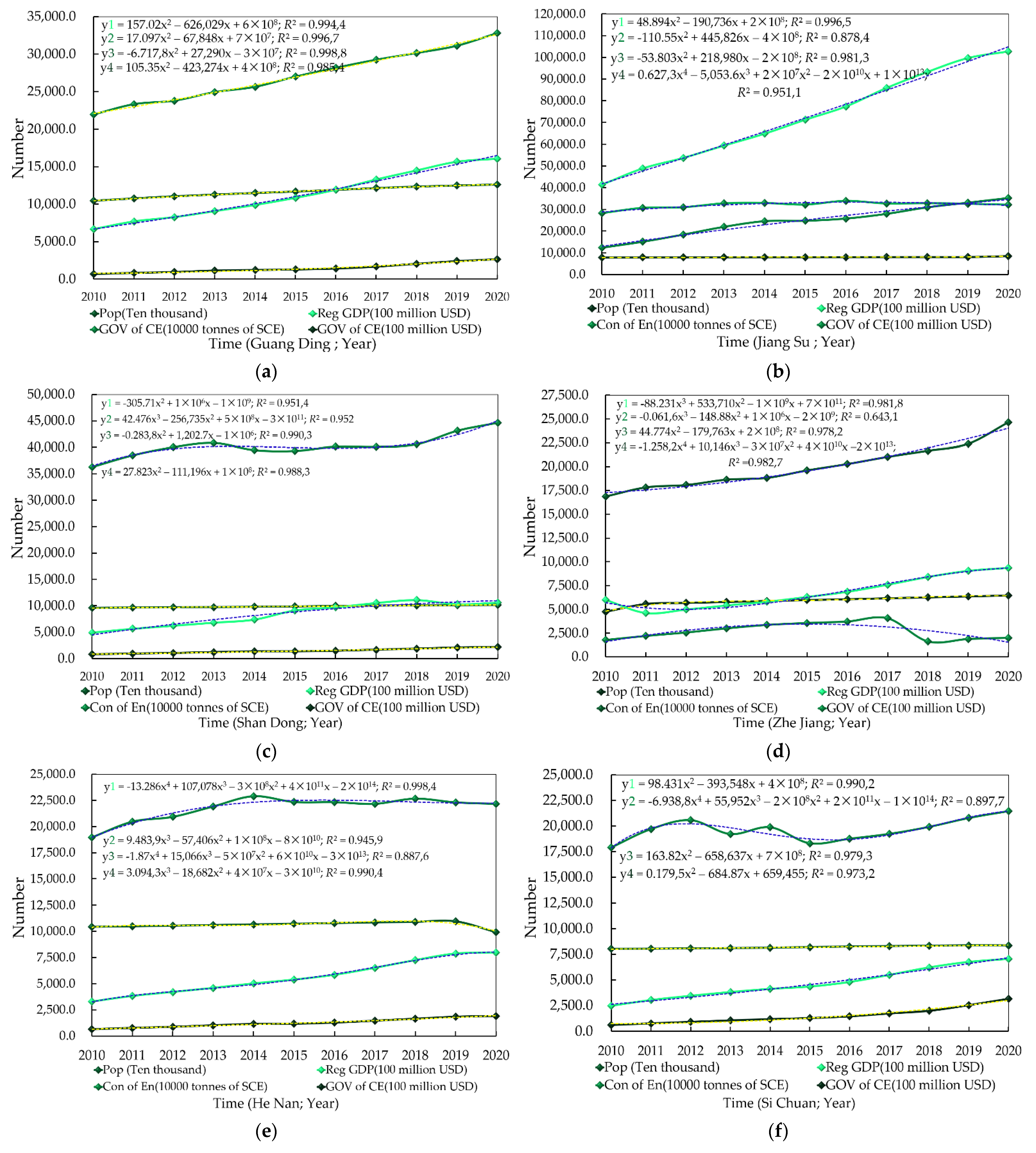
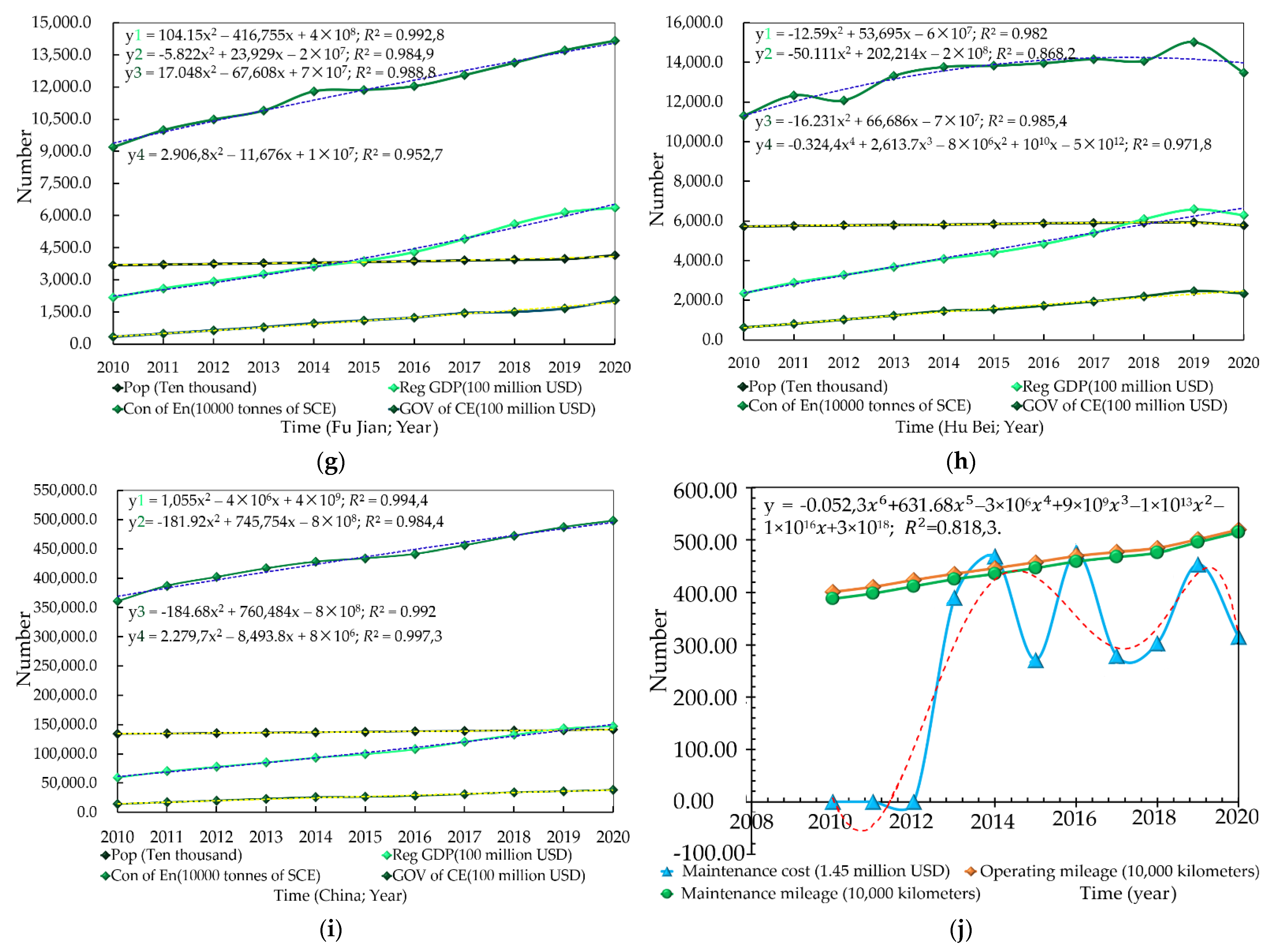
4.5. Analysis of the Construction Industry (2010~2020)

The model procedure and mathematical programming language algorithm array have been developed by the gross construction output value of the provinces obtained from Figure 5a and Equation (4) to analyze the interval sustainability by applying MATLAB [46].

4.5.1. Scientific Algorithm Model of ZWGB

The ZWGB-LCC and LCA calculation procedures are shown in Equations (2) and (3).

Other data were obtained using the same scientific algorithm.

4.5.2. Scientific Algorithm Model of XJHB, LLB, RAB, XTHB, PXHB, LSCB and EHYB

The XJHB, LLB, RAB, XTHB, PXHB, LSCB and EHYB data are obtained by using the same respective scientific algorithm, as shown in

Table 6. Sustainable impact data for the period 2010–2020.

Name	Unit (LCC: USD)	2010	2011	2012	2013	2014	2015
ZWGB	LCC (100 trillion)	6875.88	8415.92	9518.13	11,494.09	12,238.16	13,027.77
	LCA (Million t)	455.33	835.24	1208.49	2128.74	2569.68	3100.06
	SIA (100 t)	7759.14	14,232.97	20,593.44	36,275.01	43,788.89	52,826.99
XJHB	LCC (100 trillion)	1798.82	2192.75	2671.36	3188.60	3565.90	3593.87
	LCA (Million t)	180.95	327.79	592.75	1008.10	1410.02	1443.46
	SIA (Million t)	4775.69	8651.50	15,644.43	26,606.94	37,214.87	38,097.47
LLB	LCC (100 trillion)	796.77	942.73	1044.51	1208.22	1350.42	1360.32
	LCA (Million t)	125.39	207.71	282.53	437.32	610.65	624.18
	SIA (Million t)	4555.49	7546.44	10,264.93	15,888.45	22,186.04	22,677.44
RAB	LCC (100 trillion)	1770.54	2199.86	2560.07	2995.46	3359.71	3558.43
	LCA (Million t)	311.35	597.81	942.73	1510.98	2132.65	2534.29
	SIA (Million t)	837,902.23	1,608,830.25	2,537,091.09	4,066,355.16	5,739,392.57	6,820,289.57
XTHB	LCC (100 trillion)	638.08	765.49	871.30	1015.44	1147.20	1166.88
	LCA (Million t)	270.49	467.39	689.54	1092.02	1575.15	1657.70
	SIA (Million t)	72,538.32	125,342.43	184,916.69	292,849.78	422,412.80	444,551.34
PXHB	LCC (100 trillion)	609.11	769.34	912.42	1055.20	1181.51	1282.87
	LCA (Million t)	138.60	280.52	469.19	727.13	1022.10	1309.52
	SIA (Million t)	203,989.55	412,869.14	690,557.88	1,070,205.49	1,504,344.50	1,927,369.94
LSCB	LCC (100 trillion)	333.16	487.35	641.55	791.94	969.92	1102.82
	LCA (Million t)	257.64	823.31	1898.22	3593.38	6634.27	9778.27
	SIA (Million t)	10,026.31	32,040.12	73,872.36	139,843.51	258,186.95	380,543.53
EHYB	LCC (100 trillion)	629.92	810.02	1020.87	1227.47	1458.61	1535.77
	LCA (Million t)	137.38	292.57	586.36	1020.02	1712.56	1999.27
	SIA (Million t)	441.67	940.63	1885.19	3279.45	5506.06	6427.86
Name	Unit	2016	2017	2018	2019	2020	Total
ZWGB	LCC (100 t)	14,216.94	16,778.07	20,588.82	24,117.93	26,722.69	163,846.48
	LCA (t)	4029.20	6623.55	12,241.26	19,678.63	26,769.49	79,600.00
	SIA (100 t)	686.60	1128.69	2085.99	3353.36	4561.69	13,600.00
XJHB	LCC (100 trillion)	3739.73	4053.64	4488.33	4799.93	5111.37	39,149.16
	LCA (Million t)	1626.47	2071.43	2811.92	3439.20	14.67	14,900.00
	SIA (Million t)	42,927.44	54,671.42	74,215.26	90,771.21	0.025,96	394,000.00
LLB	LCC (100 trillion)	1462.64	1664.25	1870.21	2069.00	2167.31	15,949.66
	LCA (Million t)	775.91	1143.07	1622.23	2196.53	2524.78	10,600.00
	SIA (Million t)	28,190.39	41,529.98	58,938.78	79,804.17	91,730.08	383,000.00
RAB	LCC (100 trillion)	3719.74	4059.79	1621.50	1874.04	1999.57	29,724.36
	LCA (Million t)	2895.13	3764.74	239.04	369.31	448.74	15,700.00
	SIA (Million t)	7791,383.06	10,131,678.32	643,300.61	993,890.86	1,207,658.66	42,400,000.00
XTHB	LCC (100 trillion)	1277.13	1462.52	1647.24	1841.70	1902.73	13,731.21
	LCA (Million t)	2173.81	3265.48	4666.66	6523.41	7193.95	29,600.00
	SIA (Million t)	582,958.11	875,714.32	1,251,471.15	1,749,401.95	1,929,223.38	7,930,000.00
PXHB	LCC (100 trillion)	1456.37	1739.42	1994.03	2550.86	3171.09	16,674.64
	LCA (Million t)	1918.24	3272.87	4935.50	10,347.04	19,898.16	44,300.00
	SIA (Million t)	2,823,300.36	4,817,061.09	7,264,148.23	15,228,927.13	29,286,397.54	65,200,000.00
LSCB	LCC (100 trillion)	1237.03	1449.05	1503.16	1662.53	2047.03	12,223.24
	LCA (Million t)	13,829.58	22,284.98	24,888.92	33,720.83	63,097.50	181,000.00
	SIA (Million t)	538,211.08	867,275.20	968,614.39	1,312,332.01	2,455,606.32	7,040,000.00
EHYB	LCC (100 trillion)	1720.01	1941.69	2194.36	2461.99	2339.68	17,399.63
	LCA (Million t)	2809.50	4042.98	5837.23	824,597.23	707,633.22	33,800.00
	SIA (Million t)	9032.84	12,998.69	18,767.47	26,511.95	22,751.37	109,000.00

.

The research shows that the LCA emission of the eight provinces from 2010 to 2020 is:

${{\displaystyle \sum }}_{2010}^{2020}{\mathrm{LCA}}_{\mathrm{ZWGB}}$ = 79.64 billion t; ${{\displaystyle \sum }}_{2010}^{2020}{\mathrm{LCA}}_{\mathrm{XJHB}}$ = 14.93 billion t; ${{\displaystyle \sum }}_{2010}^{2020}{\mathrm{LCA}}_{\mathrm{LLB}}$ = 10.55 billion t; ${{\displaystyle \sum }}_{2010}^{2020}{\mathrm{LCA}}_{\mathrm{RAB}}$ = 15.75 billion t; ${{\displaystyle \sum }}_{2010}^{2020}{\mathrm{LCA}}_{\mathrm{XTHB}}$ = 29.58 billion t; ${{\displaystyle \sum }}_{2010}^{2020}{\mathrm{LCA}}_{\mathrm{PXHB}}$ = 44.32 billion t; ${{\displaystyle \sum }}_{2010}^{2020}{\mathrm{LCA}}_{\mathrm{LSCB}}$ = 180.81 billion t; and ${{\displaystyle \sum }}_{2010}^{2020}{\mathrm{LCA}}_{\mathrm{EHYB}}$ = 79.61 billion t, respectively.

The SIA emission relates to: ${{\displaystyle \sum }}_{2010}^{2020}{\mathrm{SIA}}_{\mathrm{ZWGB}}$ = 0.14 billion t; ${{\displaystyle \sum }}_{2010}^{2020}{\mathrm{SIA}}_{\mathrm{XJHB}}$ = 39.36 billion t; ${{\displaystyle \sum }}_{2010}^{2020}{\mathrm{SIA}}_{\mathrm{LLB}}$ = 38.33 billion t; ${{\displaystyle \sum }}_{2010}^{2020}{\mathrm{SIA}}_{\mathrm{RAB}}$ = 4237.78 billion t; ${{\displaystyle \sum }}_{2010}^{2020}{\mathrm{SIA}}_{\mathrm{XTHB}}$ = 793.14 billion t; ${{\displaystyle \sum }}_{2010}^{2020}{\mathrm{SIA}}_{\mathrm{PXHB}}$ = 6522.917 billion t; ${{\displaystyle \sum }}_{2010}^{2020}{\mathrm{SIA}}_{\mathrm{LSCB}}$ = 703.66 billion t; and ${{\displaystyle \sum }}_{2010}^{2020}{\mathrm{SIA}}_{\mathrm{EHYB}}$ = 10.86 billion t, respectively.

Fujian Province has shown the highest LCA emissions in 10 years, followed by Guangdong Province and Hubei Province (similar) and then Sichuan Province, about 24.51% of Fujian Province. However, Sichuan Province presented the highest SIA emissions, followed by Zhejiang Province and Fujian Province. The research suggests that the top three provinces in LCC do not show the highest value of LCA and SIA, disproving the many researchers’ claims that manufacturing, infrastructure, and economic growth are essential factors that cause environmental pollution.

It can be concluded that the rapid development of the economy, urbanization, and the improvement of modern industrial systems and SD are mutually restrictive and associated. They do not contradict the promotion of globalization, and it is not rapid economic development that causes environmental and social degradation.

Figure 7a compares sustainable impact data from eight provinces (from 2010 to 2020). The top three LCA emissions in 11 years are as follows: ${\mathrm{LCA}}_{2020}$ = 1270.24 billion t, ${\mathrm{LCA}}_{2019}$ = 845.21 billion t, ${\mathrm{LCA}}_{2018}$ = 572.43 billion t, and the top three years for SIA emissions are ${\mathrm{SIA}}_{2020}$ = 349,934.13 billion t, ${\mathrm{SIA}}_{2019}$ = 194,816.73 billion t, and ${\mathrm{SIA}}_{2017}$ = 168,009.40 billion t. Figure 7b refers to the biharmonic spline interpolation analysis of the mean value of sustainable data in 11 years, which shows that, after fitting, the influence of SD is increasing year by year; there were two sudden changes in 2018–2019–2020, with the growth rate exceeding 15.96%.

4.6. Establishing A Sustainable Forecast Model (2021~2108)

The Chinese government has proposed three Centennial Goals:

• Building a moderately prosperous society in all respects (GDP per capita of USD 10,503.2) 100 years after the founding of the Communist Party (1921–2021).
• They are building China into a great, modern, socialist country (GDP per capita of USD 52,700) 100 years after founding the People’s Republic of China (1949–2050).
• Turning China into a highly developed socialist country (GDP per capita of USD 85,000) after 100 years of reform and opening (1978–2078) [47,48], on which the GDP of China in 2021–2108 is analyzed. The eight provinces’ GDP and gross construction output value (2021–2108) are analyzed based on the Chinese GDP data obtained and Equation (3).

The GDP of eight provinces is estimated by analyzing an algorithm model program from 2021 to 2108 (Figure 8a), i.e., the total GDP in 88 years is 5162.99 trillion USD, in which the ranks are as follows: ${{\displaystyle \sum }}_{2021}^{2108}{\mathrm{GDP}}_{\mathrm{XJHB}}$ = 1445.11 trillion USD; ${{\displaystyle \sum }}_{2021}^{2108}{\mathrm{GDP}}_{\mathrm{ZWGB}}$ = 886.60 trillion USD; ${{\displaystyle \sum }}_{2021}^{2108}{\mathrm{GDP}}_{\mathrm{RAB}}$ = 843.52 trillion USD; ${{\displaystyle \sum }}_{2021}^{2108}{\mathrm{GDP}}_{\mathrm{XTHB}}$ = 581.00 trillion USD; ${{\displaystyle \sum }}_{2021}^{2108}{\mathrm{GDP}}_{\mathrm{PXHB}}$ = 414.45 trillion USD; ${{\displaystyle \sum }}_{2021}^{2108}{\mathrm{GDP}}_{\mathrm{LLB}}$ = 413.30 trillion USD; ${{\displaystyle \sum }}_{2021}^{2108}{\mathrm{GDP}}_{\mathrm{EHYB}}$ = 325.61 trillion USD; and ${{\displaystyle \sum }}_{2021}^{2108}{\mathrm{GDP}}_{\mathrm{LSCB}}$ = 253.40 trillion USD.

The gross construction output (CO) value of the eight provinces is 1377.34 trillion USD in total, accounting for 26.68% of the total GDP (Figure 8b).${{\displaystyle \sum }}_{2021}^{2108}{\mathrm{CO}}_{\mathrm{RAB}}$ = 394.65 trillion USD, ${{\displaystyle \sum }}_{2021}^{2108}{\mathrm{CO}}_{\mathrm{ZWGB}}$ = 304.58 trillion USD; ${{\displaystyle \sum }}_{2021}^{2108}{\mathrm{CO}}_{\mathrm{XTHB}}$ = 181.91 trillion USD; ${{\displaystyle \sum }}_{2021}^{2108}{\mathrm{CO}}_{\mathrm{XJHB}}$ = 155.69 trillion USD; ${{\displaystyle \sum }}_{2021}^{2108}{\mathrm{CO}}_{\mathrm{LSCB}}$ = 123.81 trillion USD; ${{\displaystyle \sum }}_{2021}^{2108}{\mathrm{CO}}_{\mathrm{EHYB}}$ = 114.82 trillion USD; ${{\displaystyle \sum }}_{2021}^{2108}{\mathrm{CO}}_{\mathrm{LLB}}$ = 52.16 trillion USD; and ${{\displaystyle \sum }}_{2021}^{2108}{\mathrm{CO}}_{\mathrm{PXHB}}$ = 49.73 trillion USD.

Figure 8c shows that the gross construction output value of the eight provinces is in rapid growth in the early stages of 2049, in which LSCB increases at the highest speed from 0.05% to 0.47%, and PXHB grows at a slowing pace from 0.10% to 0.11%. From 2039 to 2098, the growth rates are all down, and XJHB and PXHB tend to be stable, with only a 0.01% growth rate and a regular stage after 2098.

Figure 8d shows that the highest percentage for gross construction output value in total GDP is at 4.68–7.92% every year, followed by ZWGB (2.16–6.25%), showing that the two provinces have a higher annual investment in the construction industry. PXHB data range from 0.80% to 0.98%. In 2045, the proportion of provincial investment shows steady-state growth.

A mathematical, theoretical model Eq was established based on the data from Figure 8 to analyze the LCA and SIA values, with the sustainability analysis Eq from 2010 to 2021 being established first.

After establishing the mathematical theoretical model, the LCA values of eight provinces were analyzed by interpolation fitting for the interval 2021–2108 (Figure 9a) and values of LCA emissions of ${{\displaystyle \sum }}_{2021}^{2108}{\mathrm{LCA}}_{\mathrm{ZWGB}}$ = 788.76 billion t; ${{\displaystyle \sum }}_{2021}^{2108}{\mathrm{LCA}}_{\mathrm{XJHB}}$ = 302.19 billion t; ${{\displaystyle \sum }}_{2021}^{2108}{\mathrm{LCA}}_{\mathrm{LLB}}$ = 13.68 billion t; ${{\displaystyle \sum }}_{2021}^{2108}{\mathrm{LCA}}_{\mathrm{RAB}}$ = 95.10 billion t; ${{\displaystyle \sum }}_{2021}^{2108}{\mathrm{LCA}}_{\mathrm{XTHB}}$ = 187.79 billion t; ${{\displaystyle \sum }}_{2021}^{2108}{\mathrm{LCA}}_{\mathrm{PXHB}}$ = 52.58 billion t; ${{\displaystyle \sum }}_{2021}^{2108}{\mathrm{LCA}}_{\mathrm{LSCB}}$ = 866.72 billion t; and ${{\displaystyle \sum }}_{2021}^{2108}{\mathrm{LCA}}_{\mathrm{EHYB}}$ = 96.76 billion t.

The results show that the growth rates of LCA in eight provinces are mainly concentrated from 2021 to 2045 (Figure 9a), with an average value of over 22.05%; the lowest is ${{\displaystyle \sum }}_{2021}^{2045}{\mathrm{LCA}}_{\mathrm{RAB}}$ = 10.33%, and the highest is ${{\displaystyle \sum }}_{2021}^{2045}{\mathrm{LCA}}_{\mathrm{EHYB}}$ = 43.60%. The average growth rate from 2046 to 2108 could be about 2.11%, keeping it at the low growth stage, which shows that the environmental pollution emissions of each province have been reduced to the lowest growth.

From Figure 9b, the SIA emission values are: ${{\displaystyle \sum }}_{2021}^{2108}{\mathrm{SIA}}_{\mathrm{ZWGB}}$ = 134.41 billion t; ${{\displaystyle \sum }}_{2021}^{2108}{\mathrm{SIA}}_{\mathrm{XJHB}}$ = 208.17 billion t; ${{\displaystyle \sum }}_{2021}^{2108}{\mathrm{SIA}}_{\mathrm{LLB}}$ = 496.99 billion t; ${{\displaystyle \sum }}_{2021}^{2108}{\mathrm{SIA}}_{\mathrm{RAB}}$ = 255.91 billion t; ${{\displaystyle \sum }}_{2021}^{2108}{\mathrm{SIA}}_{\mathrm{XTHB}}$ = 50.36 billion t; ${{\displaystyle \sum }}_{2021}^{2108}{\mathrm{SIA}}_{\mathrm{PXHB}}$ = 77.39 billion t; ${{\displaystyle \sum }}_{2021}^{2108}{\mathrm{SIA}}_{\mathrm{LSCB}}$ = 337.28 billion t; and ${{\displaystyle \sum }}_{2021}^{2108}{\mathrm{SIA}}_{\mathrm{EHYB}}$ = 311.10 billion t.

4.7. Analysis the Mean Entropy Method

It is of great significance to compare the sustainable impacts of eight provinces. There are differences in geographical position, economic condition, humanistic culture, and regional government policies among the different provinces in China, showing different influences on SD [49]. A new research model (the mean entropy method) has been built to evaluate the influence of each province on the country by an analytical hierarchy process of influence factors and entropy weight method.

$$a_k={\displaystyle \sum }_n^m{\mathrm{Date}}_{\mathrm{LCA}}/\left(m-n\right), b_l=[\left(c_i-a_k\right)-\underset{1-n}{\min }{c}_m^i]/(\underset{1-n}{\max }{c}_m^j-\underset{1-n}{\min }{c}_m^i)$$

(4)

where $a_k$ is LCA average data per year for eight provinces, $n$ is nth province, $m$ is $M$^th province, $c_i$ is LCA value per year (100 million t), $\underset{1-n}{\min }{c}_m^i$ is the minimum LCA data in the same year (100 million t), and $\underset{1-n}{\max }{c}_m^j$ is the maximum LCA data in the same year (100 million t).

According to the established model formula (12), the data change laws of the eight provinces were calculated and analyzed. Figure 10a shows that the influence of the LCA mean entropy weight of the eight provinces falls into six periods, including from 2021 to 2026: ZWGB > XTHB > RAB > LSCB > XJHB > EHYB> PXHB > LLB, from 2026 to 2028: ZWGB > XTHB > LSCB > RAB > XJHB > EHYB > PXHB > LLB, from 2028 to 2034: ZWGB > LSCB > XTHB > RAB > XJHB > EHYB > PXHB > LLB, from 2034 to 2038: ZWGB > LSCB > XTHB > XJHB > RAB> EHYB > PXHB > LLB, from 2038 to 2044: ZWGB > LSCB > XJHB > XTHB > RAB > EHYB > PXHB > LLB, and from 2044 to 2108: LSCB > ZWGB > XJHB > XTHB > RAB > EHYB > PXHB > LLB.

Figure 10b presents that there are four periods for the average entropy weight of SIA of eight provinces, including RAB > ZWGB > XJHB > XTHB > EHYB > LSCB > PXHB > LLB from 2021 to 2028, RAB > LSCB > XJHB > EHYB > ZWGB > XTHB > LLB > PXHB from 2028 to 2038, LSCB > RAB > EHYB > LLB > ZWGB > XJHB > XTHB > PXHB from 2038 to 2042, and LLB > LSCB > EHYB > RAB > XJHB > ZWGB > PXHB > XTHB from 2042 to 2108.

Figure 10 refers to the LCA and SIA in eight provinces, showing a quadratic parabolic growth and monotonic linear increase with time.

5. Conclusions

China is the largest carbon emitter in the world at present. Therefore, the Chinese government has proposed and developed a series of national policies to control environmental pollution. They have also proposed reaching a carbon emission peak in 2030 and realizing zero carbon emissions by around 2060. This work will be a daunting task, especially the assessment and research on regional carbon emissions that are of great significance. The national macro goals can be realized only by ensuring that each province and region achieves the predetermined carbon emission targets.

The theoretical framework of advanced mathematical modeling and scientific algorithms is applied herein to analyze the sustainability of the construction industry in the top eight provinces of China. They were studied throughout the 21st century (2021–2108) to obtain accurate data for the three pillars of sustainability every year, including environmental, economic, and social impacts. The results show that LCA and SIA data from the eight provinces have increased, and there should be a slowed growth from 2021 to 2044. Moreover, there should be a step in the sound stage after 2045, with negative growth at a particular time. However, the overall LCA and SIA are still kept in the range of the positive interval, with no negative increase in the integrated data or decrease in total data. The result shows that the sustainability data for eight provinces will not show a zero range or harmless emissions in 2060.

The total LCC from 2021 to 2108 = 35,607,593.065 billion CNY; the average growth rate is 2.66%. The total LCA from 2021 to 2108 = 240,357.686 billion t; the average growth rate is 6.50%. The average growth rate from 2021 to 2060 is 12.53%, which is in a high growth stage. The average growth rate from 2061 to 2108 is 1.47%. The analysis data show that the environmental impact has been effectively controlled. The total SIA from 2021 to 2108 = 187,160.566 billion t; the average growth rate is 7.38%. The average growth rate from 2021 to 2060 is 14.38%, which is in a rapid growth stage. The average growth rate from 2061 to 2108 is 1.54%, and the data show that social influence has also been effectively controlled. However, LCA and SIA have yet to achieve zero or harmless emissions and are still in the low-speed growth emission stage.

The continuous growth of LCA data in the three pillars of SD will lead to excessive depletion of natural resources and severe environmental degradation. The core influencing factors of LCA are marine aquatic ecotoxicity, human toxicity, and global warming. These three are causing polar glaciers to melt and human viruses to wreak havoc and are the direct cause of global warming. The increase in SIA data will lead to the loss of community life wellbeing, increases in poverty and hunger, and the loss of peace and justice. The government needs to increase the massive investment in LCC to improve the first two. Finally, a closed-loop vicious cycle of SA→LCA↔SIA↔LCC was formed, which is also the final value embodiment of this research.

The theoretical model used in this research can be applied to evaluate the sustainability data for the construction industry in any country or region. The data obtained may provide a sufficient scientific basis for the countries and regions. Moreover, governments should develop relevant laws, regulations, rules, and short-term, medium-term, and long-term planning. The research data analysis shows that the GDP of Jiangsu, Zhejiang, and Guangdong has long ranked among the top three in China. In contrast, the LCA of Fujian Province ranks first in LCA emissions and only ranks seventh in GDP. SIA’s emission rankings are in Shandong, Fujian, and Hubei provinces. The research data disprove the conclusion of many researchers that advanced economic development is the critical factor in sustainable impact. Through the research data analysis, the authors strongly prove the urbanization process. The improvement of the modern industrial system and sustainable development are mutually restrictive and interrelated. The modern sustainable development system does not contradict the promotion of globalization.

Several problems found in the research will be further analyzed and studied. The rapid development of the economy, urbanization, and the improvement of modern industrial systems and SD are mutually restrictive and associated and will not be the cause of environmental and social degradation. The regions that rank relatively low in GDP may show relatively high values of LCA, SIA, and their influencing factors.

In the future, the authors will carry out discrete impact index analysis and optimization coupling design in this field. The research focuses on how to reduce the emissions of LCA and SIA in the construction industry and the extended application of interdisciplinary theoretical models, and it realizes the coupling design of zero-emission and harmless emission entropy weight method from the material, management, and policy aspects.

References

1. Bernstein, L.; Bosch, P.; Canziani, O.; Chen, Z.; Christ, R.; Davidson, O.; Hare, W.; Huq, S.; Karoly, D.; Kattsov, V.; et al. AR4 Climate Change 2007: Synthesis Report—IPCC. 2008. Available online: https://www.ipcc.ch/report/ar4/syr/ (accessed on 22 September 2022).
2. Edenhofer, O.; Pichs-Madruga, R.; Sokona, Y.; Agrawala, S.; Bashmakov, l.A.; Blanco, G.; Broome, J.; Bruckner, T.; Brunner, S.; Bustamante, M.; et al. AR5 Climate Change 2014: Mitigation of Climate Change—IPCC, 2015. 2015. Available online: https://www.ipcc.ch/report/ar5/wg3/ (accessed on 18 September 2022).
3. Peters, G.P.; Geden, O. Catalysing a political shift from low to negative carbon. Nat. Clim. Chang. 2017, 7, 619–621. [Google Scholar] [CrossRef]
4. Sandberg, N.H.; Brattebø, H. Analysis of energy and carbon flows in the future Norwegian dwelling stock. Build. Res. Inf. 2012, 40, 123–139. [Google Scholar] [CrossRef]
5. Scott, V.; Haszeldine, R.S.; Tett, S.F.B.; Oschlies, A. Fossil fuels in a trillion tonne world. Nat. Clim. Chang. 2015, 5, 419–423. [Google Scholar] [CrossRef] [Green Version]
6. Cui, X.; Zhao, T.; Wang, J. Allocation of carbon emission quotas in China’s provincial power sector based on entropy method and ZSG-DEA. J. Clean. Prod. 2021, 284, 124683. [Google Scholar] [CrossRef]
7. Zhou, Z.W.; Alcalá, J.; Yepes, V. Research on the optimized environment of large bridges based on multi-constraint coupling. Environ. Impact Assess. Rev. 2022, 97, 106914. [Google Scholar] [CrossRef]
8. People’s Daily. China’s Commitment to Reduce Emissions Inspires Global Climate Action. China Government Network 1. 2021. Available online: http://www.gov.cn/xinwen/2020-10/12/content_5550452.htm (accessed on 12 September 2022).
9. Duan, H.; Zhou, S.; Jiang, K.; Bertram, C.; Harmsen, M.; Kriegler, E.; van Vuuren, D.P.; Wang, S.; Fujimori, S.; Tavoni, M.; et al. Assessing China’s efforts to pursue the 1.5 °C warming limit. Science 2021, 372, 378–385. [Google Scholar] [CrossRef] [PubMed]
10. Verma, S.; Paul, A.R.; Haque, N. Selected Environmental Impact Indicators Assessment of Wind Energy in India Using a Life Cycle Assessment. Energies 2022, 15, 3944. [Google Scholar] [CrossRef]
11. Langevin, J.; Harris, C.B.; Reyna, J.L. Assessing the Potential to Reduce U.S. Building CO2 Emissions 80% by 2050. Joule 2019, 3, 2403–2424. [Google Scholar] [CrossRef] [Green Version]
12. Molina-Moreno, F.; García-Segura, T.; Martí, J.V.; Yepes, V. Optimization of buttressed earth-retaining walls using hybrid harmony search algorithms. Eng. Struct. 2017, 134, 205–216. [Google Scholar] [CrossRef]
13. Zamarrón-Mieza, I.; Yepes, V.; Moreno-Jiménez, J.M. A systematic review of application of multi-criteria decision analysis for aging-dam management. J. Clean. Prod. 2017, 147, 217–230. [Google Scholar] [CrossRef]
14. Golley, J.; Meng, X. Income inequality and carbon dioxide emissions: The case of Chinese urban households. Energy Econ. 2012, 34, 1864–1872. [Google Scholar] [CrossRef]
15. Zhou, P.; Zhang, L.; Zhou, D.; Xia, W. Modeling economic performance of interprovincial CO2 emission reduction quota trading in China. Appl. Energy 2013, 112, 1518–1528. [Google Scholar] [CrossRef]
16. Pan, X.; Teng, F.; Wang, G. Sharing emission space at an equitable basis: Allocation scheme based on the equal cumulative emission per capita principle. Appl. Energy. 2014, 113, 1810–1818. [Google Scholar] [CrossRef]
17. Tong, D.; Zhang, Q.; Zheng, Y.; Caldeira, K.; Shearer, C.; Hong, C.; Qin, Y.; Davis, S.J. Committed emissions from existing energy infrastructure jeopardize 1.5 °C climate target. Nature 2019, 572, 373–377. [Google Scholar] [CrossRef]
18. IPCC. Summary for Policymakers. In Climate Change 2014, Mitigation of Climate Change. Contribution of Working Group III to the Fifth Assessment Report of the Intergovernmental Panel on Climate Change; Cambridge University Press: Cambridge, UK, 2014. [Google Scholar] [CrossRef] [Green Version]
19. Li, Q.; Long, R.; Chen, H.; Chen, F.; Wang, J. Visualized analysis of global green buildings: Development, barriers and future directions. J. Clean. Prod. 2019, 245, 118775. [Google Scholar] [CrossRef]
20. Milani, C.J.; Yepes, V.; Kripka, M. Proposal of Sustainability Indicators for the Design of Small-Span Bridges. Int. J. Environ. Res. Public Health 2020, 17, 4488. [Google Scholar] [CrossRef] [PubMed]
21. Landi, D.; Marconi, M.; Bocci, E.; Germani, M. Comparative life cycle assessment of standard, cellulose-reinforced and end of life tires fiber-reinforced hot mix asphalt mixtures. J. Clean. Prod. 2020, 248, 119295. [Google Scholar] [CrossRef]
22. Zhou, Z.; Alcalá, J.; Yepes, V. Environmental, Economic and Social Impact Assessment: Study of Bridges in China’s Five Major Economic Regions. Int. J. Environ. Res. Public Health 2020, 18, 122. [Google Scholar] [CrossRef]
23. Zafar, M.W.; Shahbaz, M.; Sinha, A.; Sengupta, T.; Qin, Q. How renewable energy consumption contribute to environmental quality? The role of education in OECD countries. J. Clean. Prod. 2020, 268, 122149. [Google Scholar] [CrossRef]
24. Ebhota, W.S.; Tabakov, P.Y. Development of domestic technology for sustainable renewable energy in a zero-carbon emission-driven economy. Int. J. Environ. Sci. Technol. 2021, 18, 1253–1268. [Google Scholar] [CrossRef]
25. Zhou, L.; Wang, X.; Ye, A. Shake table test on transverse steel damper seismic system for long span cable-stayed bridges. Eng. Struct. 2018, 179, 106–119. [Google Scholar] [CrossRef]
26. Zhou, Z.W.; Alcalá, J.; Yepes, V. Regional sustainable development impact through sustainable bridge optimization. Structures 2022, 41, 1061–1076. [Google Scholar] [CrossRef]
27. Navarro, I.J.; Yepes, V.; Martí, J.V. Social life cycle assessment of concrete bridge decks exposed to aggressive environments. Environ. Impact Assess. Rev. 2018, 72, 50–63. [Google Scholar] [CrossRef]
28. Navarro, I.J.; Yepes, V.; Martí, J.V.; González-Vidosa, F. Life cycle impact assessment of corrosion preventive designs applied to prestressed concrete bridge decks. J. Clean. Prod. 2018, 196, 698–713. [Google Scholar] [CrossRef]
29. Penadés-Plà, V.; García-Segura, T.; Yepes, V. Accelerated optimization method for low-embodied energy concrete box-girder bridge design. Eng. Struct. 2019, 179, 556–565. [Google Scholar] [CrossRef]
30. Zhou, Z.-W.; Alcalá, J.; Kripka, M.; Yepes, V. Life Cycle Assessment of Bridges Using Bayesian Networks and Fuzzy Mathematics. Appl. Sci. 2021, 11, 4916. [Google Scholar] [CrossRef]
31. Macek, D.; Snížek, V. Innovation in Bridge Life-cycle Cost Assessment. Procedia Eng. 2017, 196, 441–446. [Google Scholar] [CrossRef]
32. Murphy, K. The social pillar of SD: A literature review and framework for policy analysis. Sustain. Sci. Pract. Policy 2012, 8, 15–29. [Google Scholar] [CrossRef] [Green Version]
33. Liu, H.; Huang, J.; Zhang, W. Numerical algorithm based on extended barycentric Lagrange interpolant for two dimensional integro-differential equations. Appl. Math. Comput. 2021, 396, 125931. [Google Scholar] [CrossRef]
34. Celik, E.; Olson, E.; Titi, E.S. Spectral Filtering of Interpolant Observables for a Discrete-in-Time Downscaling Data Assimilation Algorithm. SIAM J. Appl. Dyn. Syst. 2019, 18, 1118–1142. [Google Scholar] [CrossRef] [Green Version]
35. Tari, A.; Shahmorad, S. Differential transform method for the system of two-dimensional nonlinear Volterra integro-differential equations. Comput. Math. Appl. 2011, 61, 2621–2629. [Google Scholar] [CrossRef] [Green Version]
36. Pons, J.J.; Penadés-Plà, V.; Yepes, V.; Martí, J.V. Life cycle assessment of earth-retaining walls: An environmental comparison. J. Clean. Prod. 2018, 192, 411–420. [Google Scholar] [CrossRef]
37. Wang, Z.; Geng, L. Carbon emissions calculation from municipal solid waste and the influencing factors analysis in China. J. Clean. Prod. 2015, 104, 177–184. [Google Scholar] [CrossRef]
38. Wang, R.; Feng, W.; Wang, L.; Lu, S. A comprehensive evaluation of zero energy buildings in cold regions: Actual performance and key technologies of cases from China, the US, and the European Union. Energy 2021, 215, 118992. [Google Scholar] [CrossRef]
39. Yadollahi, M.; Nazari, R.; Spanos, N.J.; Minner, N. An application of fuzzy factor analysis for sustainable bridge maintenance and retrofit projects. Int. J. Manag. Sci. Eng. Manag. 2017, 12, 225–236. [Google Scholar] [CrossRef]
40. China, National Development and Reform Commission. Notice on Further Liberalizing the Price of Professional Services for Construction Projects (Fagai Price [2015] No.299). National Development and Reform Commission of China 1. 2015. Available online: https://www.ndrc.gov.cn/xxgk/zcfb/tz/202009/t20200927_1239632.html (accessed on 16 September 2022).
41. China, National Development and Reform Commission. Notice of the State Planning Commission of China and the Ministry of Construction on Issuing the Regulations on the Management of Engineering Survey and Design Fees.National Development and Reform Commission of China 1. 2002. Available online: https://services.ndrc.gov.cn/ecdomain/portal/portlets/bjweb/newpage/answerconsult/interactivepage.jsp?itemcode=&idseq=c244918bca3c49fa97ff044f9bd39293&code=&state=123 (accessed on 13 September 2022).
42. China, Ministry of Transport of the People’s Republic. Highway Engineering Budget Estimates, Quotas, Standards, and Reforms. Ministry of Transport of the People’s Republic of China 100. 2018. Available online: https://xxgk.mot.gov.cn/2020/jigou/glj/202103/t20210331_3547339.html (accessed on 25 September 2022).
43. Marti-Vargas, J.R.; Ferri, F.J.; Yepes, V. Prediction of the transfer length of prestressing strands with neural networks. Comput. Concr. 2013, 12, 187–209. [Google Scholar] [CrossRef]
44. Zhou, N.; Khanna, N.; Feng, W.; Ke, J.; Levine, M. Scenarios of energy efficiency and CO2 emissions reduction potential in the buildings sector in China to year 2050. Nat. Energy. 2018, 3, 978–984. [Google Scholar] [CrossRef]
45. Hao, Y.; Wang, Y.; Wu, Q.; Sun, S.; Wang, W.; Cui, M. What affects residents’ participation in the circular economy for SD? Evidence from China. Sustain. Dev. 2020, 28, 1251–1268. [Google Scholar] [CrossRef]
46. Shaker, A.; Abouelatta, M.; Sayah, G.T.; Zekry, A. Comprehensive physically based modelling and simulation of power diodes with parameter extraction using MATLAB. IET Power Electron. 2014, 7, 2464–2471. [Google Scholar] [CrossRef]
47. Yanbin, C.; Wei, L. China’s Economic Growth and High_Quality Development: 2020–2035. China Econ. 2021, 16, 1–17. [Google Scholar] [CrossRef]
48. Hu, A.; Yan, Y.; Tang, X.; Liu, S. 2050 China: Strategic Goals and Two Stages. In 2050 China. Understanding Xi Jinping’s Governance; Springer: Singapore, 2021; pp. 45–60. [Google Scholar] [CrossRef]
49. Liu, J.; Diamond, J. China’s environment in a globalizing world. Nature 2005, 435, 1179–1186. [Google Scholar] [CrossRef] [PubMed]
Figure 1. Cluster coupling data analysis and location display.
Sustainability 14 16645 g001
Figure 2. Three-dimensional curve diagram analysis of thin plate spline (the eight countries of the top).
Sustainability 14 16645 g002
Figure 3. The theoretical framework and system of SD.
Sustainability 14 16645 g003
Figure 4. Mathematical models analysis of relevant data: (a) China; (b) Shan Dong.
Sustainability 14 16645 g004
Figure 5. Relevant data analysis of eight provinces and maintenance costs: (a) Guang Dong (b) Jiang Su (c) Shan Dong (d) Zhe Jiang (e) He Nan (f) Si Chuan (g) Fu Jiang (h) Hu Bei (i) China (j) 2010–2020 maintenance costs per kilometer.
Sustainability 14 16645 g005aSustainability 14 16645 g005b
Figure 6. Analysis data of bridges: (a) ratio of LCC, LCA and SIA; (b) analysis of polynomial fit.
Sustainability 14 16645 g006
Figure 7. Analysis data from the provinces (2010~2020): (a) date analysis of LCC and LCA; (b) date analysis of LAC and SIA.
Sustainability 14 16645 g007
Figure 8. Analysis data for eight provinces (2021~2108): (a) GDP date; (b) total construction output value; (c) ratio of total construction output value per year to GDP per year; (d) ratio of the total construction output value of each province in each year to the total GDP of the eight provinces in that year.
Sustainability 14 16645 g008aSustainability 14 16645 g008b
Figure 9. Analysis data from eight provinces (2021~2108): (a) LCA date; (b) SIA date.
Sustainability 14 16645 g009
Figure 10. Analysis data from eight provinces (2021~2108): (a) LCA date; (b) model of LCC-LCA.
Sustainability 14 16645 g010