
Modeling Pedestrian Detour Behavior By-Passing Conflict Areas
Abstract
:1. Introduction
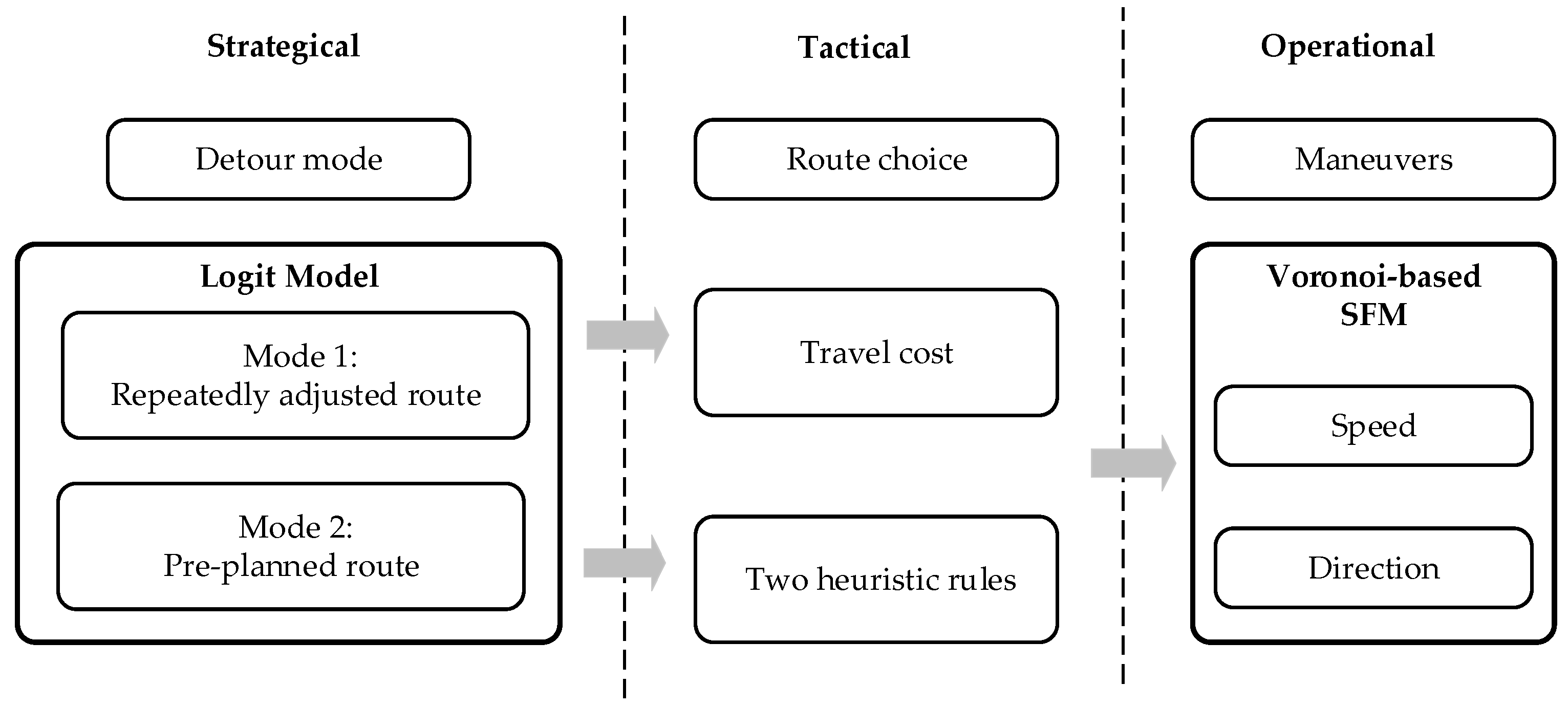
2. Model
2.1. Strategic Layer Model
2.2. Tactical Layer Model
2.2.1. Group That Repeatedly Adjust Routes during the Trip
2.2.2. Group That Pre-Plan Route before Walking or during the Initial Period of the Trip
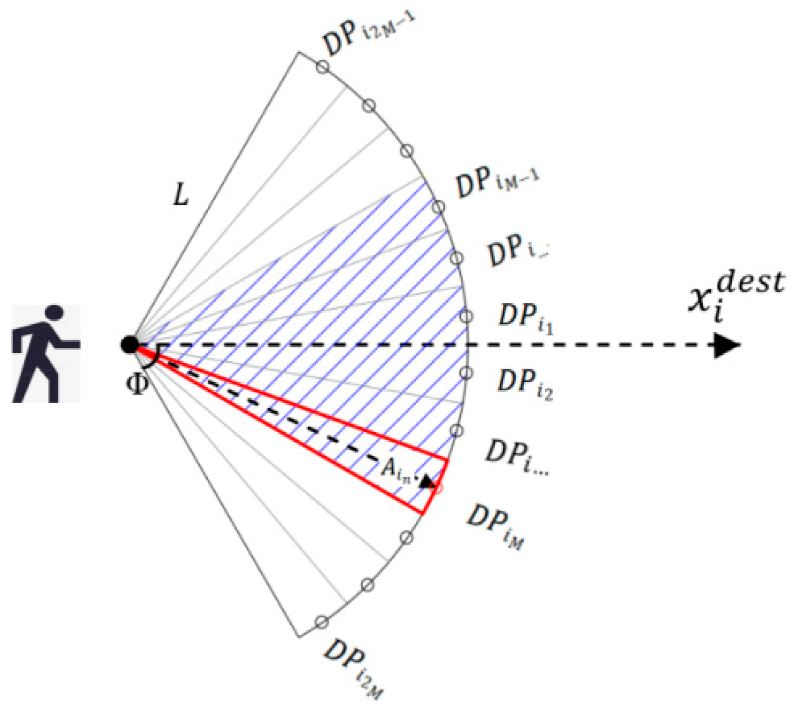
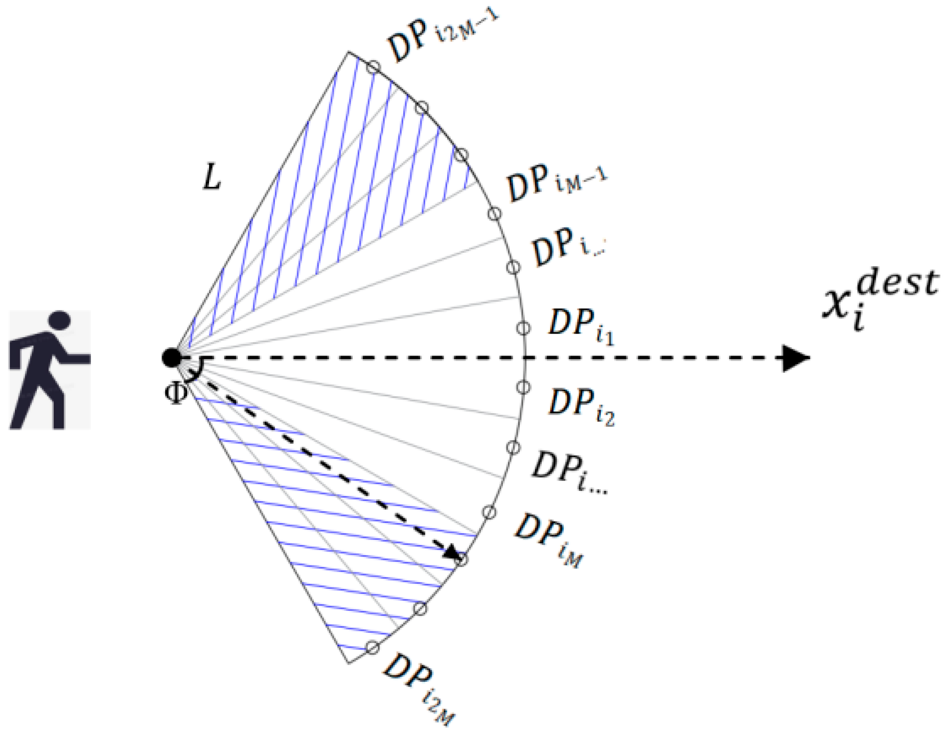
2.3. Operational Layer Model
2.3.1. Movement Speed
2.3.2. Movement Direction
3. Experimental Data Analysis
3.1. Experiment Setting
3.2. Model Evaluation Indexes
3.3. Detour Statistical Characteristics
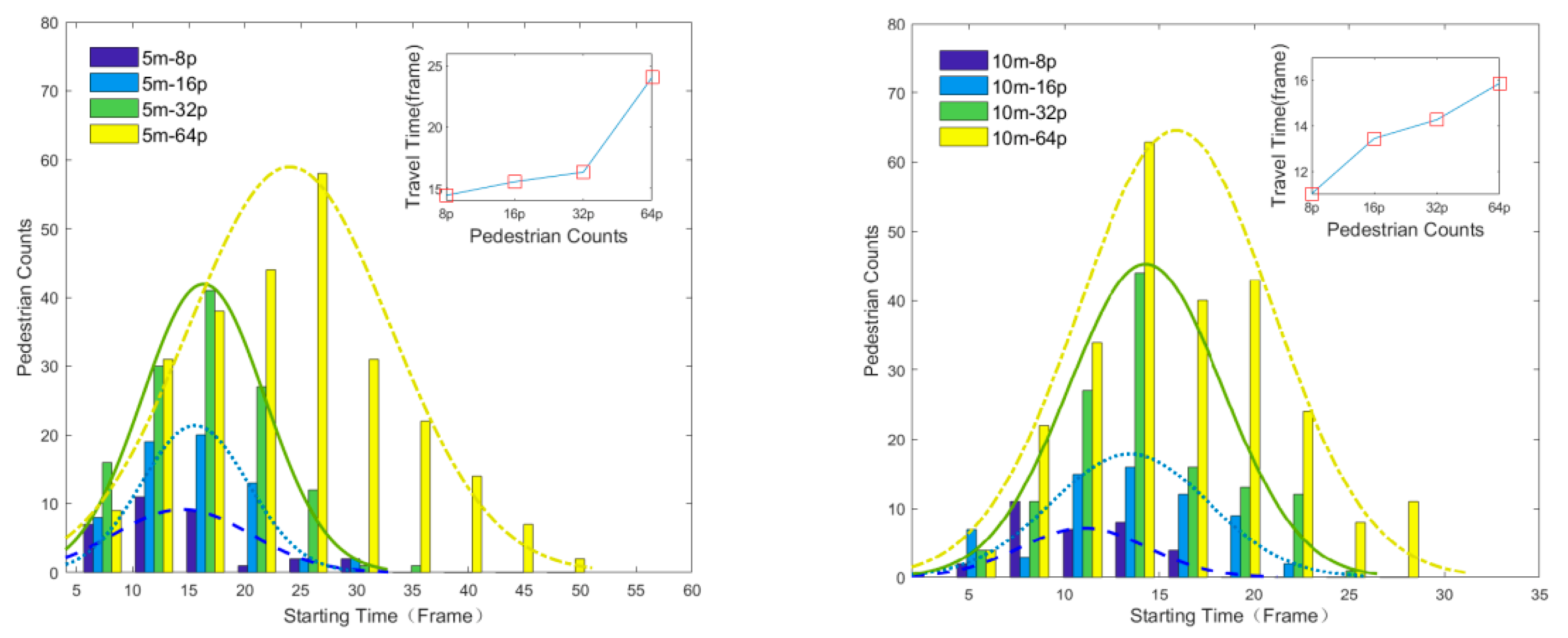
3.3.1. Starting Time
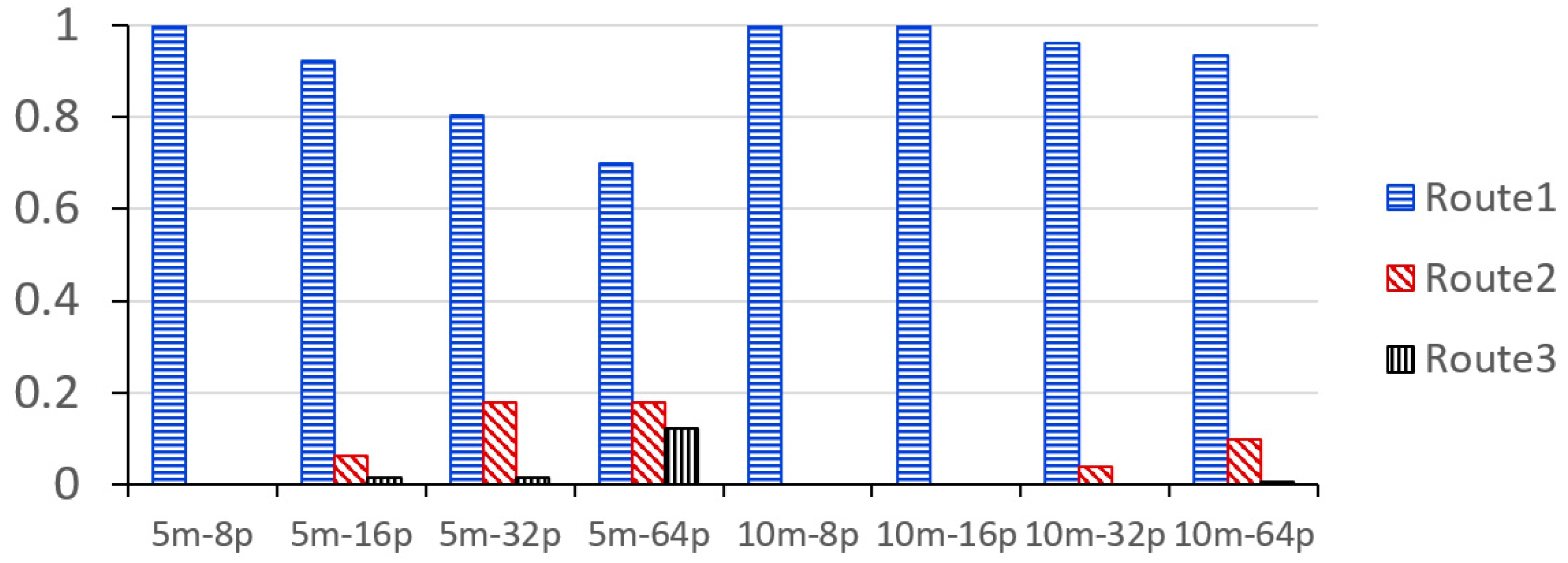
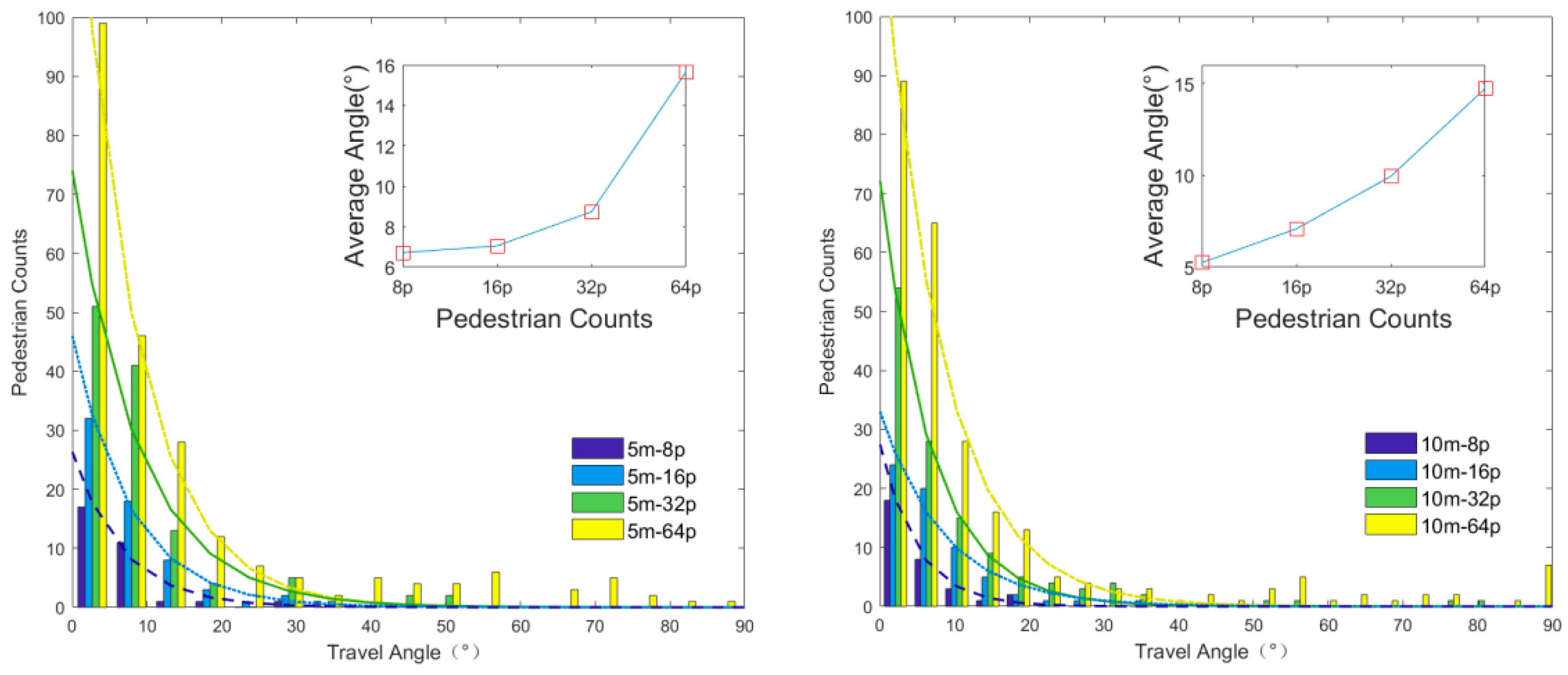
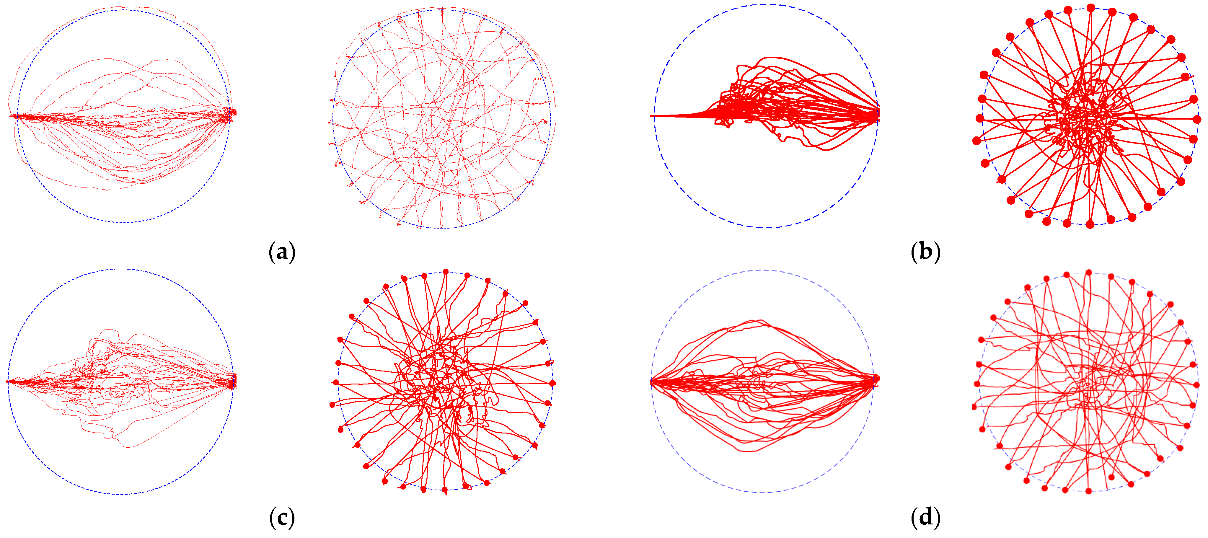
3.3.2. Detour Mode and Angle
4. Simulation Experiment
4.1. Parameter Setting and Simulation Results
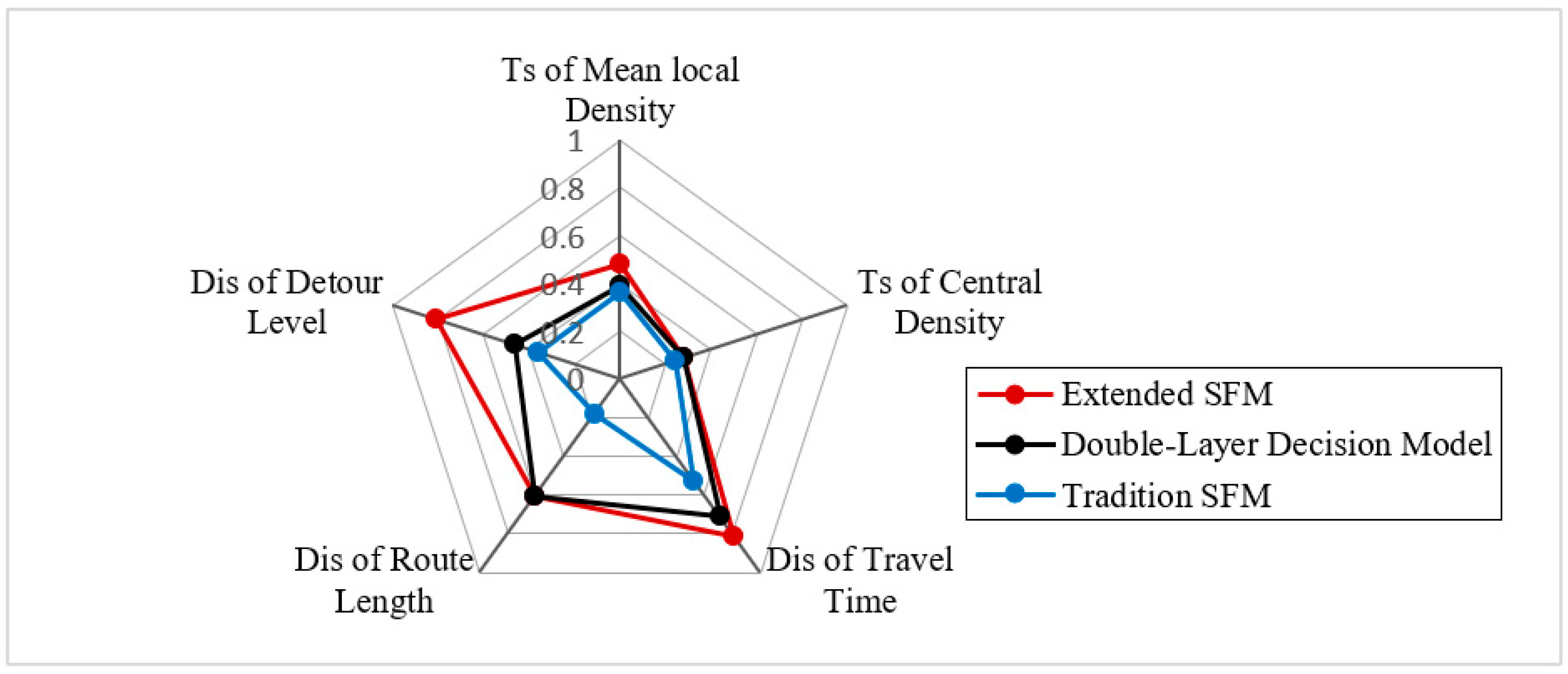
4.2. Model Evaluation
5. Conclusions
- (1)
- In reality, pedestrians may switch or combine the two movement modes of “repeatedly adjusting the route during the trip” and “pre-planning the route before walking or during the first period of the trip”, which is not considered in this paper. In the future, we will continue to explore whether the path decision-making modes of pedestrians have changed in the process of moving from one place to another, which has not received much attention so far.
- (2)
- Pedestrians are directly divided into two groups at the starting position for different walking guidance, without considering the dynamic time difference of pedestrians making this large-scale detour decision. In fact, this decision is made before the trip or during the initial period of the trip, and there is a certain time difference.
- (3)
- In fact, the speed of movement depends on the quality of the road and the landform. The tendency of pedestrians to avoid conflict areas is related to the individual characteristics of pedestrians. In the future, we will further study the influence of road quality, terrain and individual characteristics on pedestrians’ walking speed, and detour tendency.
Author Contributions
Funding
Institutional Review Board Statement
Informed Consent Statement
Data Availability Statement
Conflicts of Interest
References
- Saadatseresht, M.; Mansourian, A.; Taleai, M. Evacuation planning using multiobjective evolutionary optimization approach. Eur. J. Oper. Res. 2009, 198, 305–314. [Google Scholar] [CrossRef]
- Yang, L.; Ping, R.; Zhu, K.; Liu, S.; Xin, Z. Observation study of pedestrian flow on staircases with different dimensions under normal and emergency conditions. Saf. Sci. 2012, 50, 1173–1179. [Google Scholar] [CrossRef]
- Hughes, R.L. A continuum theory for the flow of pedestrians. Transp. Res. Part B Methodol. 2002, 36, 507–535. [Google Scholar] [CrossRef]
- Dressler, D.; Gro, M.; Kappmeier, J.P.; Kelter, T.; Kulbatzki, J.; Plümpe, D.; Schlechter, G.; Schmidt, M.; Skutella, M.; Temme, S. On the use of network flow techniques for assigning evacuees to exits. Procedia Eng. 2010, 3, 205–215. [Google Scholar] [CrossRef] [Green Version]
- Abdelghany, A.; Abdelghany, K.; Mahmassani, H. A hybrid simulation-assignment modeling framework for crowd dynamics in large-scale pedestrian facilities. Transp. Res. Part A Policy Pract. 2016, 86, 159–176. [Google Scholar] [CrossRef]
- Blue, V.J.; Adler, J.L. Cellular automata microsimulation for modeling bi-directional pedestrian walkways. Transp. Res. Part B Methodol. 2001, 35, 293–312. [Google Scholar] [CrossRef]
- Zhou, X.M.; Hu, J.J.; Ji, X.F.; Xiao, X.Z.Y. Cellular automaton simulation of pedestrian flow considering vision and multi-velocity. Phys. A Stat. Mech. Appl. 2019, 514, 982–992. [Google Scholar] [CrossRef]
- Helbing, D. Social force model for pedestrian dynamics. Phys. Rev. E 1995, 51, 4282. [Google Scholar] [CrossRef] [Green Version]
- Haghani, M.; Sarvi, M. Simulating pedestrian flow through narrow exits. Phys. Lett. A 2019, 383, 110–120. [Google Scholar] [CrossRef]
- Fiorini, P.; Shiller, Z. Motion Planning in Dynamic Environments Using Velocity Obstacles. Int. J. Robot. Res. 1998, 17, 760–772. [Google Scholar] [CrossRef]
- Masood, K.; Molfino, R.; Zoppi, M. Simulated Sensor Based Strategies for Obstacle Avoidance Using Velocity Profiling for Autonomous Vehicle FURBOT. Electronics 2020, 9, 883. [Google Scholar] [CrossRef]
- Antonini, G.; Bierlaire, M.; Weber, M. Discrete choice models of pedestrian walking behavior. Transp. Res. Part B Methodol. 2006, 40, 667–687. [Google Scholar] [CrossRef]
- Hoogendoorn, S.P.; Bovy, P.H.L. Pedestrian route-choice and activity scheduling theory and models. Transp. Res. Part B Methodol. 2004, 38, 169–190. [Google Scholar] [CrossRef]
- Farina, F.; Fontanelli, D.; Garulli, A.; Giannitrapani, A.; Prattichizzo, D. Walking Ahead: The Headed Social Force Model. PLoS ONE 2017, 12, e0169734. [Google Scholar] [CrossRef] [PubMed] [Green Version]
- Li, W.; Gong, J.; Yu, P.; Shen, S.; Li, R.; Duan, Q. Simulation and analysis of congestion risk during escalator transfers using a modified social force model. Phys. A Stat. Mech. Appl. 2015, 420, 28–40. [Google Scholar] [CrossRef]
- Moussaid, M.; Helbing, D.; Theraulaz, G. How simple rules determine pedestrian behavior and crowd disasters. Proc. Natl. Acad. Sci. USA 2011, 108, 6884–6888. [Google Scholar] [CrossRef] [Green Version]
- Yuen, J.K.K.; Lee, E.W.M. The effect of overtaking behavior on unidirectional pedestrian flow. Saf. Sci. 2012, 50, 1704–1714. [Google Scholar] [CrossRef]
- Hoogendoorn, S.P.; Van Wageningen-Kessels, F.L.M.; Daamen, W.; Duives, D.C. Continuum modelling of pedestrian flows: From microscopic principles to self-organised macroscopic phenomen. Phys. A Stat. Mech. Appl. 2014, 416, 684–694. [Google Scholar] [CrossRef]
- Xiao, Y.; Gao, Z.; Qu, Y.; Li, X. A pedestrian flow model considering the impact of local density: Voronoi diagram based heuristics approach. Transp. Res. Part C Emerg. Technol. 2016, 68, 566–580. [Google Scholar] [CrossRef]
- Qu, Y.; Xiao, Y.; Wu, J.; Tang, T.; Gao, Z. Modeling detour behavior of pedestrian dynamics under different conditions. Phys. A Stat. Mech. Appl. 2018, 492, 1153–1167. [Google Scholar] [CrossRef]
- Li, M.; Shu, P.; Xiao, Y.; Wang, P. Modeling detour decision combined the tactical and operational layer based on perceived density. Phys. A Stat. Mech. Appl. 2021, 574, 126021. [Google Scholar] [CrossRef]
- Guo, N.; Hao, Q.-Y.; Jiang, R.; Hu, M.-B.; Jia, B. Uni- and bi-directional pedestrian flow in the view-limited condition: Experiments and modeling. Transp. Res. Part C Emerg. Technol. 2016, 71, 63–85. [Google Scholar] [CrossRef]
- Hoogendoorn, S.P.; Van Wageningen-Kessels, F.; Daamen, W.; Duives, D.C.; Sarvi, M. Continuum theory for pedestrian traffic flow: Local route choice modelling and its implications. Transp. Res. Part C Emerg. Technol. 2015, 59, 183–197. [Google Scholar] [CrossRef]
- Abraham, J.E.; Hunt, J.D. Random utility location, production, and exchange choice; Additive Logit model; and spatial choice microsimulations. Transp. Res. Rec. 2007, 2003, 1–6. [Google Scholar] [CrossRef]
- Park, B.U.; Simar, L.; Zelenyuk, V. Nonparametric estimation of dynamic discrete choice models for time series data. Comput. Stat. Data Anal. 2017, 108, 97–120. [Google Scholar] [CrossRef] [Green Version]
- Lovreglio, R.; Fonzone, A.; Dell’olio, L. A mixed logit model for predicting exit choice during building evacuations. Transp. Res. Part A Policy Pract. 2016, 92, 59–75. [Google Scholar] [CrossRef]
- Steffen, B.; Seyfried, A. Methods for measuring pedestrian density, flow, speed and direction with minimal scatter. Phys. A Stat. Mech. Appl. 2010, 389, 1902–1910. [Google Scholar] [CrossRef] [Green Version]
- Luo, L.; Liu, X.B.; Fu, Z.J.; Ma, J.; Liu, F.X. Modeling following behavior and right-side-preference in multidirectional pedestrian flows by modified FFCA. Phys. A Stat. Mech. Appl. 2020, 550, 124149. [Google Scholar] [CrossRef]
- Ling, H.; Wong, S.C.; Zhang, M.; Shu, C.W.; Lam, W. Revisiting Hughes’ dynamic continuum model for pedestrian flow and the development of an efficient solution algorithm. Transp. Res. Part B 2009, 43, 127–141. [Google Scholar]
- Kretz, T.; Lehmann, K.; Hofs, I.; Leonhardt, A. Dynamic Assignment in Microsimulations of Pedestrians. arXiv 2014, arXiv:1401.1308. [Google Scholar]
- Parisi, D.R.; Gilman, M.; Moldovan, H. A modification of the Social Force Model can reproduce experimental data of pedestrian flows in normal conditions. Phys. A Stat. Mech. Appl. 2009, 388, 3600–3608. [Google Scholar] [CrossRef]
- Xiao, Y.; Gao, Z.; Jiang, R.; Li, X.; Qu, Y.; Huang, Q. Investigation of pedestrian dynamics in circle antipode experiments: Analysis and model evaluation with macroscopic indexes. Transp. Res. Part C Emerg. Technol. 2019, 103, 174–193. [Google Scholar] [CrossRef]
- Huang, S.S.; Wei, R.C.; Lo, S.M.; Lu, S.X.; Li, C.H.; An, C.; Liu, X.X. Experimental study on one-dimensional movement of luggage-laden pedestrian. Phys. A Stat. Mech. Appl. 2019, 516, 520–528. [Google Scholar] [CrossRef]
- Bera, A.; Kim, S.; Manocha, D. Online parameter learning for data-driven crowd simulation and content generation. Comput. Graph. 2016, 55, 68–79. [Google Scholar] [CrossRef]
- Helbing, D.; Buzna, L.; Johansson, A.; Werner, T. Self-organized pedestrian crowd dynamics: Experiments, simulations, and design solutions. Transp. Sci. 2005, 39, 1–24. [Google Scholar] [CrossRef]


| Experiment | p-Value | |||
|---|---|---|---|---|
| 8p | 16p | 32p | 64p | |
| 5 m | 0.4288 | 0.6495 | 0.3389 | 0.1354 |
| 10 m | 0.1411 | 0.1376 | 0.6501 | 0.5860 |
| Experiment | p-Value | |||
|---|---|---|---|---|
| 8p | 16p | 32p | 64p | |
| 5 m | 0.2536 | 0.4734 | 0.3045 | 0 |
| 10 m | 0.6189 | 0.6992 | 0.1688 | 0 |
| Independent Variables | B | S.E. | Wald | Sig. | Exp(B) |
|---|---|---|---|---|---|
| 0.189 | 0.063 | 9.085 | 0.000 | 1.208 | |
| 0.228 | 0.057 | 16.093 | 0.000 | 1.256 | |
| −6.613 | 1.346 | 24.136 | 0.000 | 0.001 |
| Parameter | Value | Parameter | Value |
|---|---|---|---|
| 12 | |||
| 1.58953 | 0.004 | ||
| 0.29 s | |||
| 0.26 | 2.78 | ||
| 1 |
Publisher’s Note: MDPI stays neutral with regard to jurisdictional claims in published maps and institutional affiliations. |
© 2022 by the authors. Licensee MDPI, Basel, Switzerland. This article is an open access article distributed under the terms and conditions of the Creative Commons Attribution (CC BY) license (https://creativecommons.org/licenses/by/4.0/).
Share and Cite
Ning, Q.; Li, M. Modeling Pedestrian Detour Behavior By-Passing Conflict Areas. Sustainability 2022, 14, 16522. https://doi.org/10.3390/su142416522
Ning Q, Li M. Modeling Pedestrian Detour Behavior By-Passing Conflict Areas. Sustainability. 2022; 14(24):16522. https://doi.org/10.3390/su142416522
Chicago/Turabian StyleNing, Qingyan, and Maosheng Li. 2022. "Modeling Pedestrian Detour Behavior By-Passing Conflict Areas" Sustainability 14, no. 24: 16522. https://doi.org/10.3390/su142416522