Spatial Spillover Effects of Agricultural Agglomeration on Agricultural Non-Point Source Pollution in the Yangtze River Basin

Abstract

Agricultural non-point source pollution has become a matter of increasing public concern, and modern agriculture is gradually transforming into agglomeration, so it is important to study the influence of agricultural agglomeration on agricultural non-point source pollution to coordinate the relationship between resources, environment, and agricultural economic growth for guidance. With a focus on 89 prefecture-level cities in the main agricultural production areas of the Yangtze River basin in China, the authors analyzed the spatial and temporal evolution trends of agricultural agglomeration and agricultural non-point source pollution from 2000 to 2020 and then empirically tested the spatial spillover effects of agricultural agglomeration on agricultural non-point source pollution based on the spatial Durbin model (SDM). The results show that: (1) Between 2000 and 2020, agricultural agglomeration, in general, decreased from 0.364 to 0.342, and cities with agglomeration values in the third and fourth ranks are mainly located in the area north of the Yangtze River and have a tendency to extend southward over time. Agricultural non-point source pollution shows a general trend of increasing and then decreasing; its emissions rose from 404.319 × 10⁴ tons in 2000 to 464.341 × 10⁴ tons in 2015, and then fell to 373.338 × 10⁴ tons in 2020, emissions in the third and fourth class of cities are mainly located in the middle and lower basin of the Yangtze River; High-value hots-pot areas of agricultural agglomeration, that is, areas with high spatial correlation, are mainly located in the upper and lower Yangtze River basin, and the areas with the higher spatial correlation of agricultural non-point source pollution are distributed in the upper, middle and lower basin of the Yangtze River. (2) The whole basin and upper basin exhibit positive and negative spatial spillover effects of agricultural non-point source pollution, Spillover effects values are 0.300 and −1.086, respectively; Agricultural agglomeration of the Whole Basin has a positive direct effect and a negative spatial spillover effect on agricultural non-point source pollution, the effect values are 0.846 and −0.520, respectively. (3) In addition to the core explanatory variable, agricultural production conditions and the share of livestock and poultry industry have a positive direct effect (the effect values are 0.109 and 0.048, respectively) and a negative spatial spillover effect (the effect values are −0.520 and −0.910, respectively) on agricultural non-point source pollution, while agricultural population size has a positive direct effect and spatial spillover effect, the effect values 0.099 and 0.452 respectively; The urbanization rate exacerbates the emission of agricultural non-point source pollution, the effect value is 0.110. while the industrial structure reduces the emission of agricultural non-point source pollution, the effect value is −0.438, but neither has a spatial spillover effect. The results imply that some effective policy measures, such as strengthening research on nutrient requirements and fertilization techniques for major crops, improving farmland infrastructure, scientifically planning and monitoring the scale of livestock farms, and strengthening inter-regional coordination and cooperation in the fight against pollution, should be taken to achieve ecological and sustainable objectives.

1. Introduction

Over the past 40 years since the reform and opening, China’s agriculture has made remarkable achievements under the real dilemma of having more people and less land. Statistics show that in 2021, the added value of the primary industry was 830.86 billion yuan, and the total grain production was 671 million tons, which was twice as much as that in 1978 at the beginning of the reform and opening, achieving the “17 consecutive bumper crop”. However, due to the constraints of arable land, water resources, and the level of agricultural science and technology, the rough use of large amounts of chemical fertilizers, pesticides, and agricultural plastic films has produced agricultural non-point source pollution (ANP), which has a wide range of impacts, is difficult to control and lasts for a long time, while enhancing the economic benefits of agriculture. In 2020, the “Second National Pollution Source Census Bulletin” shows that agricultural non-point source pollution emissions: 10.6713 million tons of chemical oxygen demand, 1.4149 million tons of total nitrogen, 0.2120 million tons of total phosphorus, respectively, accounting for 49.8%, 46.5%, 67.2% of total water pollutant emissions, total agricultural non-point source pollution emissions are at a high level. In March 2021, the Ministry of Ecology and Environment, Ministry of Agriculture and Rural Affairs jointly issued the “agricultural surface source pollution management and supervision and guidance implementation plan (Trial run)” pointed out that by 2025, the key areas of agricultural non-point source pollution will be initially controlled, the layout of agricultural production will be further optimized, the amount of fertilizer and pesticide application will be significantly reduced, the level of comprehensive utilization of manure and sewage from livestock and poultry farms below the scale will continue to improve, green development of agriculture will achieve significant results.

In the meantime, modern agriculture is shifting from crude, disorderly and scattered characteristics to intensive, specialized, and agglomeration. That is to say; agricultural production activities constantly agglomerate in a region. However, agricultural agglomeration has positive and negative externalities on the ecological environment. On the one hand, Agricultural agglomeration will bring about the Scale economy effect of agriculture, and the specialized division of labor and collaboration brought about by economies of scale can save operating costs, helping to reduce the input of chemical-based production elements and stimulating farmers to adopt green energy-saving technologies, thereby reducing the emissions of agricultural non-point source pollution. On the other hand, agricultural agglomeration will bring about the diffusion and spillover of agriculture-related knowledge and technology. Farmers will be motivated to choose livestock and poultry farming with high risks, high returns, and high pollution, plus agricultural agglomeration will make pollutants largely gather in a region, which will intensify the emission of agricultural non-point source pollution. In general, the final effect of agricultural agglomeration on the ecological environment is the result of the mutual game between positive and negative environmental externalities. Therefore, in promoting modern agriculture characterized by scale and intensification, it is of practical significance to clarify the relationship between agricultural agglomeration and agricultural non-point source pollution to realize agriculture’s green economic transformation.

The current research on industrial agglomeration, agricultural agglomeration, and environmental pollution has been widely studied by domestic and foreign scholars from different perspectives. Firstly, studies on industrial agglomeration mainly involve the definition of the concept of industrial agglomeration by Marshall [1], Weber [2], Schumpeter [3], Hoover [4], Porter [5]; the reasons for the formation of industrial agglomeration, such as spatial costs [6], regional house price differences [7], and marketization [8]; the regional economic effects of industrial agglomeration, such as promoting technological progress [9], optimizing resource allocation [10], and reducing pollution emissions [11]; and the measurement of industrial agglomeration, such as the Herfindahl index [12], concentration index [13], Gini coefficient [14], and locational entropy index [15]. Secondly, studies on agricultural agglomeration mainly concern: the causes of agricultural agglomeration formation, including the improvement of technology and human capital [16,17], technology exchange [18], demonstration and learning effects [19], and artificial intelligence [20]; the spatial and temporal evolutionary trends of agricultural agglomeration [21,22,23,24]; and the economic effects of agricultural agglomeration, including promoting the economic growth of agricultural industries [25,26,27], facilitating labor productivity [28,29], boosting agricultural industrialization [30], and advancing the income level of farmers [31]. Finally, research on agricultural non-point source pollution mainly involves sources of agricultural non-point source pollution, including chemical fertilizers, pesticides, agricultural plastic films, livestock and poultry manure, and domestic waste [32]; hazards of agricultural non-point source pollution, including soil nutrient loss [33], eutrophication of water bodies [34], and degradation of atmospheric quality [35]; quantitative measurement of agricultural non-point source pollution, including the mean pollution concentration method [36], comprehensive survey method [37], inventory analysis method [38], and unit analysis method [39]; and influencing factors of agricultural non-point source pollution, including urbanization, industrial structure, fiscal policy, financial policy, and income level of rural residents [40,41].

However, there is still some debate on the relationship between industrial agglomeration and environmental pollution. The reason is that there are positive and negative effects of industrial agglomeration on environmental pollution, and the final result depends on the final game between the two sides, thus, the relationship between the two sides is uncertain, with three different views: First, industrial agglomeration will slow down environmental pollution, and the economies of scale brought by industrial agglomeration will improve the production efficiency and management level of enterprises and reduce the cost of pollution control per unit of output. In addition, the spillover of knowledge and technology generated by industrial agglomeration will also reduce pollution emissions, thus improving regional environmental quality [42,43,44,45]. Secondly, industrial agglomeration will aggravate environmental pollution, and industrial agglomeration will aggravate pollutant emissions through the expansion of the industrial scale, the admission of highly polluting industries, and the accumulation of pollutants [46,47,48,49]. Thirdly, the effect of industrial agglomeration on environmental pollution is uncertain; there may be an “N,” inverted “N” [50], “U” [51], and inverted “U” [52] type relationship between industrial agglomeration and environmental pollution. However, most of the existing studies focus on the relationship between industrial agglomeration and industrial pollution, and only a small amount of literature concerns the study of the relationship between agricultural agglomeration and agricultural non-point source pollution, such as some scholars focused on planting and farming industries and empirically examined the relationship between agricultural agglomeration and agricultural non-point source pollution [53,54].

By collating and summarizing the existing studies domestic and foreign scholars have conducted extensive and in-depth studies on industrial agglomeration and agricultural non-point source pollution. Specifically, it discusses the evolution trend of industrial agglomeration, the reasons for its formation, the economic effect of agglomeration, and the measurement of agglomeration, resulting in rich theoretical achievements. Secondly, it deeply studies the harm, measurement methods, and influencing factors of agricultural non-point source pollution, enriching the relevant theoretical and practical achievements of agricultural non-point source pollution. Thirdly, regarding the exploration of the effect of agricultural agglomeration on agricultural non-point source pollution, a large amount of existing literature focuses on the environmental pollution effect of industrial agglomeration. Only a small amount of literature focuses on the environmental pollution effect of agricultural agglomeration. Its research conclusions are not unified, which are roughly divided into three aspects: industrial agglomeration will slow down environmental pollution, industrial agglomeration will aggravate environmental pollution, and the effect of industrial agglomeration on environmental pollution is uncertain. Although existing research has resulted in a wealth of findings, there are some shortcomings. The existing studies on the environmental pollution effects of industrial agglomeration mostly focus on industry, and even if they focus on agriculture, they mostly focus on leading agricultural enterprises, the agricultural products processing industry, and the farming industry, lacking relevant studies on agricultural primary products. Moreover, the existing studies mostly focus on the national or provincial level, lacking attention to specific main agricultural production areas. Furthermore, agriculture non-point source pollution can seep into the recipient water bodies through surface or underground runoff. Therefore, agricultural non-point source pollution has a certain fluidity and diffusivity; that is, agricultural non-point source pollution in one area will affect the surrounding area while existing studies are less likely to explore the spatial spillover effect of agricultural agglomeration on agricultural non-point source pollution.

Therefore, this paper takes the main agricultural production areas in the Yangtze River basin as the research are, and takes “plantation” and “farming,” which have the largest proportion of agricultural non-point source pollution output, as the research objects. Based on the data at the prefectural level from 2000 to 2020, we measured and analyzed the emissions of agricultural non-point source pollution and the level of agricultural agglomeration in the Yangtze River basin using the inventory analysis, Gini coefficient, and the average industrial agglomeration rate, and empirically investigated the direct effect of agricultural agglomeration on agricultural non-point source pollution and the spatial spillover effect based on the spatial econometric model, The purpose is to address the following issues: (1) What is the status of agricultural non-point source pollution emissions in the Yangtze River Basin? What are the differences in agricultural non-point source pollution emissions in different areas in the upper, middle and lower basin of the Yangtze River? (2) What is the effect of agricultural agglomeration on agricultural non-point source pollution in the Yangtze River Basin? Does it intensify or slow down? (3) Since the economic base, natural conditions, and resource endowment differ greatly between the upper, middle, and lower basins of the Yangtze River basin, and thus, the impact of agricultural agglomeration on agricultural non-point source pollution also differs to some extent. (4) Since agricultural non-point source pollution has a certain diffusivity, does agricultural agglomeration have a certain spatial spillover effect on agricultural non-point source pollution in the Yangtze River basin? The findings based on the above empirical analysis can provide recommendations for preventing and controlling agricultural non-point source pollution in the Yangtze River Basin and coordinating resources, environment, and agricultural economic growth.

2. Materials and Methods

2.1. Materials

2.1.1. Spatial Weights Matrix

A spatial weight matrix must be constructed before spatial econometric analysis can be performed. In order to consider both economic and geographical factors, this paper constructs an economic-geographic nested matrix. The specific calculation formula is as follows.

$$W=W_d\times diag\left(\overline{x_1}/\overline{x}, \overline{x_2}/\overline{x}, \dots \dots \overline{x_i}/\overline{x}\right)$$

(1)

where $W_d$ is the Inverse distance matrix, its elements are represented by the inverse of the geographical distance between the two cities; $diag\left(\overline{x_1}/\overline{x}, \overline{x_2}/\overline{x}, \dots \dots \overline{x_i}/\overline{x}\right)$ denotes the diagonal matrix; Where $\overline{x_i}/\overline{x}$ is diagonal elements, $\overline{x}$ and $\overline{x_i}$ represents the per capita gross regional product of all regions and region $i$ in the main agricultural production areas of the Yangtze River basin from 2000 to 2020, respectively.

2.1.2. Moran’s I Statistic

Before spatial econometric analysis, the original data needs to be tested for spatial correlation, and if there is a spatial correlation in the original data, the spatial econometric model can be used to analyze the empirical results; otherwise, the traditional standard measurement method will be used. Based on the research theme, this paper first uses the global Moran’s I index to test the spatial correlation of agricultural non-point source pollution in each prefecture-level city in the main agricultural production area of the Yangtze River basin. The global Moran’s I index calculation formula is as follows.

$$\mathrm{Moran}’\mathrm{s}\mathrm{I}=\frac{{{\displaystyle \sum }}_{i=1}^n{{\displaystyle \sum }}_{i=1}^n{W}_{ij}(Y_i-\overline{Y})(Y_j-\overline{Y})}{S^2{{\displaystyle \sum }}_{i=1}^n{{\displaystyle \sum }}_{i=1}^n{W}_{ij}}$$

(2)

$S^2=\frac{1}{n}{\displaystyle \sum }_{i-1}^n(Y_i-\overline{Y}{)}^2$ is the variance of agricultural non-point source pollution. n is the number of samples ($n=89$), $W_{ij}$ ($i,j=1,2,\dots ,n$) is the element of the spatial weight matrix $W$. $\overline{Y}=\frac{1}{n}{\displaystyle \sum }_i^n{Y}_i$, $Y_i$ is the agricultural non-point source pollution of the unit $i$. The Moran’s I Statistic has a value range of −1 to 1. The more this statistic converges to 1, the stronger the positive spatial correlation of the agricultural non-point source pollution, Otherwise, the more this statistic converges to −1, the stronger the negative spatial correlation of the agricultural non-point source pollution.

2.2. Variable Definitions and Data Description

2.2.1. Dependent Variable

Measurement Method

The explanatory variable in this paper is agricultural non-point source pollution (NPS). Based on the object of study-planting and farming, this paper first selects chemical fertilizer, solid farm waste, and livestock farming as the agricultural non-point source pollution sources to be measured in this paper. This results in 14 accounting units (

Table 1. Accounting units for agricultural non-point source pollution.

Pollution Source	Pollution Unit	Measurement Method
Fertilizer	Nitrogen fertilizer, phosphate fertilizer, compound fertilizer	Total nitrogen emissions = (nitrogen fertilizer refined amount + compound fertilizer refined amount × 15%) × nitrogen loss coefficient Total phosphorus emissions = (phosphorus fertilizer refined amount + compound fertilizer refined amount × 15%) × 43.66% × nitrogen loss coefficient
Agricultural solid waste	Rice, wheat, vegetables, beans, oilseeds, potatoes, corn	Crop/vegetable production × waste output coefficient × nutrient content × Utilization Structure × emission rate under specific utilization structure
Livestock and poultry farming	Pigs, cattle, sheep, poultry	Livestock and poultry breeding volume × daily excretion coefficient of manure and urine × feeding cycle × contaminant content of manure and urine × manure and urine loss rate

), including fertilizers (nitrogen fertilizers, phosphate fertilizers, compound fertilizers), agricultural solid waste (rice, wheat, corn, beans, potatoes, oilseeds, vegetables), livestock and poultry farming (pigs, cattle, sheep, poultry), and the pollutants produced mainly include four categories of TN (total nitrogen), TP (total phosphorus), NH₃N (ammonia nitrogen) COD (chemical oxygen demand). Then the pollution production process is analyzed, the loss factor of each pollution accounting unit is determined by the quantitative analysis of the pollution loss from each non-point source, and the loss factor of each pollution unit is determined mainly by consulting various literature. Finally, we use the inventory analysis method to account for agricultural non-point source pollution. The specific calculation formula is as follows.

$$\begin{gathered} E={\displaystyle \sum }_{i}E{U}_i{\rho }_i\left(1-{\eta }_i\right)C_i\left(E{U}_i,S\right) \\ ={{\displaystyle \sum }}_{i}P{E}_i\left(1-{\eta }_i\right)C_i\left(E{U}_i,S\right) \end{gathered}$$

(3)

where $E$ is the total amount of emissions; $E{U}_i$ is the statistic of unit $i$; ${\rho }_i$ is the coefficient of pollution generation of unit $i$; ${\eta }_i$ is the coefficient of resource use efficiency in the agricultural production process; $P{E}_i$ is the amount of pollution production of unit $i$, that is the maximum potential pollution after deducting resource use and management factors, containing pollutants that enter the water body, do not enter the water body, and are self-purified. $C_i$ is the emission coefficient of unit $i$, It is influenced by the pollution accounting unit “$EU$” and the spatial characteristics of the area “$S$”, and can be used to characterize the effects of weather, hydrology, regional environment and various management measures on pollution.

The Description of the Relevant Coefficients of Each Pollution Unit

1. Fertilizer pollution unit: The main agricultural production area in the Yangtze River basin spans the east and west of China, covering a large area with a complex and diverse natural environment. Therefore the loss coefficient of fertilizer should be different. This paper uses the First National Pollution Source Census-Fertilizer Loss Coefficient Manual for Agricultural Pollution Sources and refers to the established literature to determine the fertilizer loss coefficients for each province (city) in the main agricultural production areas of the Yangtze River Basin (

Table 2. Nitrogen and phosphorus fertilizer loss coefficients by province and city/%.

Region	Nitrogen Fertilizer Loss Coefficient	Phosphorus Fertilizer Loss Coefficient	Phosphorus Fertilizer Loss Coefficient	Nitrogen Fertilizer Loss Coefficient	Phosphorus Fertilizer Loss Coefficient
Shanghai	1.271	0.589	Shanghai	1.056	0.375
Jiangsu	0.946	0.385	Jiangsu	1.081	0.366
Zhejiang	1.179	0.351	Zhejiang	0.776	0.396
Anhui	1.131	0.495	Anhui	1.052	0.399
Jiangxi	1.062	0.578	Jiangxi

). The loss coefficient of each prefecture-level city refers to the loss coefficient of its province (city), and ammonia nitrogen emissions from fertilizer sources are estimated at 8.3% of total nitrogen production [55].

2. Solid farmland waste pollution unit: Agricultural solid wastes mainly include straw and vegetables. Since these agricultural solid wastes are rich in nitrogen, phosphorus, and organic matter, and their long-term stockpiling will cause non-point source pollution by flowing to rivers with rainwater, this paper determines the calculation of pollutant emissions from agricultural solid wastes based on the application of the non-point source pollution assessment method by S. Yun Lai (2004) [39] (Table 1). The coefficients involved include straw to grain ratio of crops (

Table 3. Ratio of straw to grain of major crops/%.

Crop Type	Rice	Wheat	Corn	Beans	Potatoes	Oilseeds
Straw/Grain	97	103	137	171	61	226

), nutrient content of crops and vegetables (

Table 4. Nutrient content of solid waste from various crops and vegetables/%.

Crop Type	Nutrient Content
	COD	TN	TP
Rice	0.58	0.6	0.04
Wheat	0.62	0.5	0.09
Corn	0.82	0.78	0.17
Beans	1.03	1.3	0.13
Potatoes	0.37	0.3	0.11
Oilseeds	0.91	2.01	0.14
Vegetables	1.00	0.18	0.09

), utilization structure (

Table 5. Regional straw utilization structure %.

Projects	Fertilizer	Feed	Fuel	Raw Materials	Incineration	Stacking
Sichuan	14.3	22.8	53.6	2.7	3	3.6
Chongqing	14.3	22.8	53.6	2.7	3	3.6
Hubei	38	11.8	46.4	2.9	0	0.9
Hunan	71	17.69	6.8	0.31	2.2	2
Jiangxi	65.1	17.7	11.8	1.4	2	2
Anhui	30.3	31.8	17.5	2.9	14.6	2.9
Jiangsu	31.9	13.2	33.9	5.8	7.2	8

), and loss rate under specific utilization structure (

Table 6. Loss rate under specific utilization structure/%.

Projects		Fertilizer	Feed	Fuel	Raw Materials	Incineration	Stacking
utilization structure		31.9	13.2	33.9	5.8	7.2	8
loss rate under specific utilization structure/%	COD	20	0	0	0	0	50
	TN	15	0	0	0	0	50
	TP	5	0	0	0	10	50

). In addition, the waste generation rates of different vegetable species varied widely, and the average value of 1.47 was taken in this paper. NH₃N emissions from agricultural solid waste were still estimated as 8.3% of the total nitrogen generation.

3. Livestock and poultry breeding: This paper determines the coefficients involved in livestock and poultry farming pollution units based on the Survey of Pollution in the National Scale Livestock and Poultry Farming Industry and Countermeasures for Prevention and Control prepared by the Department of Natural Ecological Protection of the State Environmental Protection Administration [56], including the feeding cycle and daily excretion coefficient of livestock and poultry (

Table 7. Manure and urine excretion coefficient and feeding cycle of livestock and poultry.

Projects	Unit	Pigs	Cattle	Sheep	Poultry
Manures	kg/day	2.000	20.000	2.600	0.125
	kg/year	398.000	7300.000	950.000	26.250
Urine	kg/day	3.300	10.000	—	—
	kg/year	656.700	3650.000	—	—
Feeding cycle	day	199.000	365.000	365.000	210.000

), the average content of pollutants (

Table 8. Pollutant content of livestock manure and urine on average (kg/t).

Projects	COD	NH3N	TP	TN
Pig manure	52.000	3.08	3.410	5.880
Pig urine	9.000	1.43	0.520	3.300
Cow manure	31.000	1.71	1.180	4.370
Cow urine	6.000	3.47	0.400	8.000
Sheep manure	4.630	0.8	2.600	7.500
Poultry manure	45.700	2.8	5.800	10.400

), and the pollutant loss coefficient (

Table 9. Manure and urine loss coefficient of livestock and poultry.

Projects	Pig Manure	Pig Urine	Cow Manure	Cow Urine	Sheep Manure	Poultry Manure
loss coefficient	8%	35%	8%	35%	8%	20%

).

2.2.2. Independent Variable

The core explanatory variable in this paper is the level of agricultural agglomeration (AGG). Based on the previous theoretical analysis, this paper first measures the level of agricultural agglomeration in the whole Yangtze River basin agricultural main production area from 2000 to 2020 using the Gini coefficient and then measures the level of agricultural agglomeration in each prefecture-level city in the main agricultural production area of the Yangtze River basin using average industrial agglomeration rate.

(1) Gini coefficient: The Gini coefficient was originally used to measure the degree of imbalance, and agricultural agglomeration is also a phenomenon of uneven distribution of industries, so the Gini coefficient can be used to measure the overall degree of regional agricultural agglomeration. In this study, a simple and easy-to-use Gini coefficient is used to measure the degree of agricultural agglomeration in the main agricultural regions of the Yangtze River basin. The specific calculation formula is as follows.

$$G=1-\frac{1}{n}(2{{\displaystyle \sum }}_{i=1}^{n-1}{L}_i+1)$$

(4)

where $G$ is the Agricultural Gini coefficient. $n$ is the number of groups grouped equally in the prefecture-level city of the main agricultural production areas of the Yangtze River basin, the Gini coefficient ranges from 0 to 1, with larger values indicating that the distribution of industries tends to be more clustered.

(2) Average industrial agglomeration rate: This paper adopts the average regional industrial agglomeration rate to obtain the degree of agricultural agglomeration in each prefecture-level city. This method directly measures the average occupancy rate of all industries in a specific region, and the higher its occupancy share, the higher the degree of industrial concentration in the region. Furthermore, because this study needs to measure the integrated agglomeration level of planting and farming, the measured value of this index can truly reflect the spatial distribution of agricultural agglomeration level, and the calculation formula is as follows.

$$V_i=\frac{1}{m}{{\displaystyle \sum }}_{j=1}^m\frac{Y_{ij}}{Y_j}$$

(5)

$V_i$ is the average agricultural agglomeration rate of city $i$; $\mathrm{m}$ is the number of types of agricultural products, $Y_{ij}$ is the production of agricultural products $j$ in city $i$, $Y_j$ is the production of agricultural product $j$ in the main agricultural regions of the Yangtze River basin, The higher the value of $V_i$, the higher the degree of agricultural agglomeration in the prefecture-level city.

2.2.3. Control Variable

In order to improve the accuracy of the model estimation, factors that can influence agricultural non-point source pollution are selected as control variables to be included in the model in this paper, and with reference to existing studies, the selection of control variables is as follows.

(1) Agricultural production conditions (APC): The continuous improvement of agricultural production conditions not only helps to improve the efficiency of the utilization and allocation of elements but also enables the resource utilization of waste generated in the process of agricultural production, such as resource utilization of crop straw and biogas processing of livestock and poultry manure, thus reducing the load of pollutants on the environment. At the same time, with the continuous improvement of agricultural production conditions, pollutants are also generated, such as the irrational use of chemical fertilizers can bring about the loss of nitrogen, phosphorus, and other pollutants, thus posing a threat to the environment. In this paper, the measurement of agricultural production conditions mainly involves four aspects of agricultural mechanization, electrification, water conservancy, and chemistry [57], specifically using the combined values of seven indicators measured by the entropy method, namely, fertilizer application, pesticide use, agricultural plastic film, the total power of agricultural machinery, rural electricity consumption, agricultural diesel use, and effective irrigation area, to characterize agricultural production conditions.

(2) Agricultural population size (APS): Agricultural production in a region cannot be achieved without the participation of people, so the size of the agricultural population also has an impact on the environment; the larger the size of the agricultural population in a region indicates a corresponding increase in production and consumption activities in the region, with production activities generating solid waste from farmland, loss of fertilizers, and irrational use of livestock and poultry manure, and consumption activities generating human feces and urine and domestic sewage [58]. The study of agricultural non-point source pollution in this paper focuses on farming, livestock, and poultry industries; it does not include agricultural non-point source pollution from human feces, urine, and domestic sewage. Therefore, this paper uses the ratio of agricultural, forestry, and fishery workers to rural workers multiplied by 100% to measure the agricultural population size (APS).

(3) Livestock and poultry industry structure (LPS): The research objective of this paper focuses on planting and farming, which have different pollution emission intensities and characteristics. However, the differences in the share of farming and livestock between different regions mean that the emissions of agricultural non-point source pollution vary from region to region [59]. Therefore, this paper characterizes the structure of the livestock and poultry industry (LPS) by the total output value of the livestock and poultry industry/total output value of agriculture, forestry, animal husbandry, and fishing industries.

(4) Urbanization Rate (UR): The urbanization rate not only represents the level of urbanization of a region but also reflects the level of modernization of a region. In addition, changes in the urbanization rate reflect changes in population structure, which in turn cause changes in rural production and consumption behavior and ultimately impact the agroecological environment [60]. Therefore, this paper uses the urban resident population/total population × 100% to characterize the urbanization rate. Since the resident urban population is not counted in some regions, the urban household population is used as a substitute.

(5) Industrial Structure (IS): Developing secondary and tertiary industries helps increase farmers’ non-farm income, relaxes their financial constraints, and allows them to keep more funds remaining. It can be used to acquire green agricultural production equipment, thus improving the ecological environment. Moreover, increased remaining funds will allow the restructuring of rural industries. Farmers may be more inclined to engage in relatively higher-risk livestock and poultry farming. This restructuring of agricultural production will also impact the rural ecological environment due to the differences in the characteristics and intensity of pollutant production in livestock farming and planting [61]. The restructuring of agricultural production will also have an impact on the rural ecological environment because of the differences in the characteristics and intensity of pollutant production from livestock farming and planting. Therefore, this paper takes the ratio of the sum of values added by secondary and tertiary industries to the sum added by primary, secondary, and tertiary industries to measure the industrial structure.

Based on the above definitions of the dependent variable, independent variable, and control variable,

Table 10. Variable definitions.

Types	Symbol	Variables	Variable Definition
Dependent Variable	NPS	Agricultural Non-Point Source Pollution	Summed from COD, NH3N, TN, TP (Ten thousand tons)
Independent Variable	AGG	Agricultural Aggregation	Average agricultural agglomeration rate
Control Variable	APC	Agricultural Production Conditions	Combined scores of agricultural chemistry, mechanization, hydrology, and electrification
	APS	Agricultural Population size	(Agriculture, forestry, animal husbandry and fishery workers divided by rural workers) × 100 (%)
	AHS	Livestock and Poultry Industry Structure	(Total output value of livestock industry divided by total output value of agriculture, forestry, animal husbandry and fishery) × 100 (%)
	UR	Urbanization Rate	(Urban resident population divided by total population) × 100 (%)
	IS	Industry Structure	(Value added of secondary and tertiary industries divided by value added of primary, secondary and tertiary industries) × 100 (%)

represents the assignment and Explanation of variables. In addition, in order to reduce the effect of heteroscedasticity and avoid errors in the data caused by differences in units or magnitudes of variables, the natural logarithm of each variable involved in the model is taken in this paper to make the data more smooth, and the measurement results more reliable.

Table 11. Description of variables between 2000 and 2020.

Variables	Obs	Mean	Std.	Min	Max
lnNPS	1869	1.247	0.807	−1.434	3.309
lnAGG	1869	3.891	0.171	1.839	4.43
lnAPC	1869	−2.327	1.214	−11.513	−0.367
lnAPS	1869	3.888	0.375	2.298	4.59
lnAHS	1869	3.416	0.407	0.909	4.619
lnUR	1869	3.677	0.445	2.05	4.464
lnIS	1869	4.423	0.112	3.878	4.595

represents the description of each variable.

2.3. Study Area and Data Source

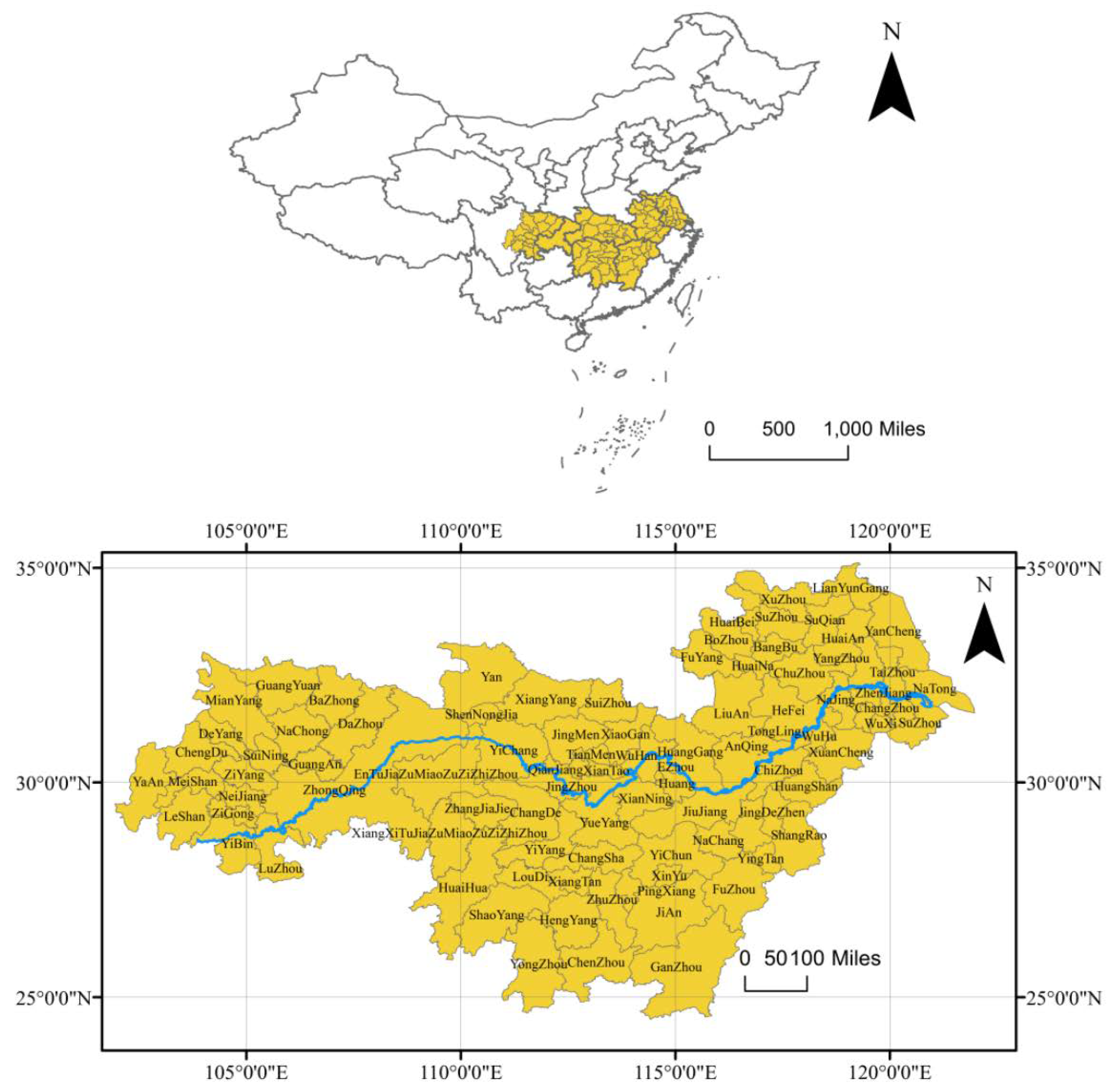
2.3.1. Study Area

The Yangtze River Basin is one of the seven major agricultural production areas in China, covering the upper, middle, and lower basins of the Yangtze River, with a high-quality rice industry belt, a dedicated wheat industry belt, a high-quality cotton industry belt, a high-quality rape industry belt, a livestock industry belt and an aquatic products industry belt, owning rich in diverse agricultural and livestock resources. However, the Yangtze River basin also faces more serious ecological and environmental problems. Therefore, as a basic sector of the national economy, it is also necessary to actively implement the concept of “ecological priority and green development.” In light of this, this paper focuses on the “main agricultural production areas in the Yangtze River Basin.” Based on the distribution of various agricultural and livestock products in the main agricultural production areas of the Yangtze River basin, seven provinces (cities) in Sichuan, Chongqing, Hubei, Hunan, Jiangxi, Anhui, and Jiangsu were selected as the sample study areas, and focus on the prefecture-level city level. Since the agricultural share of Aba Tibetan and Qiang Autonomous Prefecture, Ganzi Tibetan Autonomous Prefecture, Liangshan Yi Autonomous Prefecture, and Panzhihua City in Sichuan Province is relatively small; these four areas are excluded from the prefecture-level cities in Sichuan Province; thus the sample study area contains a total of 89 prefecture-level cities, as shown in Figure 1 (101°37′–121°57′ E 23°52–36°4′ N). In addition, the main agricultural production areas in the Yangtze River basin are divided into three major regions: the upper basin, including Sichuan Province and Chongqing City; the middle basin, including Hubei Province, Hunan Province, and Jiangxi Province; and the lower basin, including Anhui Province and Jiangsu Province.

2.3.2. Data Source

The data for this study are mainly obtained from the statistical yearbooks and statistical bulletins of each prefecture-level city or municipality, the China Urban Statistical Yearbook, the China Rural Statistical Yearbook, the National Bureau of Statistics, and the EPS database. For missing data from some years, the interpolation method is used to supplement them. For the missing data of a certain indicator in a certain region, this paper adopts the average share or average value of the province where the region is located to supplement them to ensure the integrity and reliability of the overall data.

3. Results and Discussion

3.1. Spatial and Temporal Evolutionary Trends of Agricultural Agglomeration and Agricultural Non-Point Source Pollution

3.1.1. Temporal Change Trends of Agricultural Agglomeration and Agricultural Non-Point Source Pollution

The Gini coefficient and inventory analysis were used to measure agricultural agglomeration and agricultural non-point source pollution in the main agricultural production areas of the Yangtze River basin from 2000 to 2020 and to divide the main agricultural production areas of the Yangtze River basin into three regions: upper, middle and lower basin, and to plot the temporal trends of agricultural agglomeration and agricultural non-point source pollution in the whole basin, upper, middle and lower basin from 2000 to 2020, as shown in Figure 2 and Figure 3.

Firstly, Figure 2 depicts the trend of agricultural agglomeration over time. By comparing the level of agricultural agglomeration in the three sub-basins, it can be seen that the level of agricultural agglomeration is highest in the lower basin, followed by the middle basin, and the smallest in the lower basin, while the level of agricultural agglomeration in the whole basin is lower than that in the lower basin until 2010 and greater than that in the lower basin region after 2010. This indicates that the agricultural agglomeration levels in the upper, middle, and lower basins of the main agricultural production areas in the Yangtze River basin exhibit unbalanced characteristics, which is generally consistent with the current distribution pattern of economic development levels in the upper, middle and lower basins of the Yangtze River basin [62]. The best economic development level is in the lower basin, followed by the middle basin, and the worst in the upper basin. The higher the level of economic development, the higher the degree of feedback to agriculture; therefore, the agricultural economic development levels in the upper, middle, and lower basins largely show the same pattern; as the level of agricultural economic development increases, the higher the degree of agricultural modernization, large-scale operation, and, thus agricultural agglomeration. In addition, the middle and lower basins are flatter than the upper basin, creating better conditions for large-scale agricultural operations and thus, higher levels of agricultural agglomeration. From the evolutionary trend of agricultural agglomeration in the whole basin and the three sub-basins during 2000–2020, agricultural agglomeration, in general, decreased from 0.364 to 0.342, and except for the upper basin, the level of agricultural agglomeration in the whole basin, the middle basin, and the lower basin show a decreasing trend in general, and the upper basin shows a decreasing and then increasing trend. The possible reason is that with the introduction of China’s western development and the Belt and Road policy, the upper basin, represented by Chongqing and Sichuan, has enjoyed more policy dividends from the state, prompting their agricultural development level to increase and narrowing their agricultural agglomeration level with the middle and lower basin.

Figure 3 depicts the trend of agricultural non-point source pollution over time. By comparing the agricultural concentration levels in the three sub-basins, it can be seen that agricultural non-point source pollution emissions are highest in the middle basin, followed by the lower basin, and smallest in the upper basin. From the trend of agricultural non-point source pollution in each region over time, the emissions of agricultural non-point source pollution in the upper reach and lower reach do not fluctuate significantly and are roughly in the range of 0.8–1.5 million tons. The upper reach is mainly located in the western region of China, restricted by its geographical conditions; agricultural production is mostly characterized by agriculture, and the degree of large-scale operation is relatively low, making the emissions of agricultural non-point source pollution in the region relatively small. Meanwhile, the lower reach is mainly located in the eastern coastal region of China, and the level of economic development is relatively superior, which can provide high-quality agricultural production resources and human resources for the development of modern agriculture. In contrast, the emissions of agricultural non-point source pollution in the middle basin show a trend of rising and falling, reaching a maximum value in 2015 with emissions of 2.3 million tons. The trend of agricultural non-point source pollution emissions in the whole basin is largely consistent with that in the middle basin, also reaching a maximum value of 4.6 million tons in 2015, which indicates that the emissions of agricultural non-point source pollution in the main agricultural regions of the Yangtze River basin and the temporal trends are mainly determined by the middle reach. The reason for this is that the flat terrain, dense water network, and superior climate in the middle basin are more suitable for the growth of crops and livestock breeding so that agricultural production resources continue to gather in the region, both for cultivation and livestock, which, together with the fact that modern green agricultural production methods have not yet replaced the current industrialization of agricultural production, makes the emissions of agricultural non-point source pollution per unit area also rise [63].

3.1.2. Spatial Distribution of Agricultural Agglomeration and Agricultural Non-Point Source Pollution

In this paper, based on the agricultural agglomeration level (AGG) and agricultural non-point source pollution emissions (NPS) of the prefecture-level cities in the main agricultural production areas of the Yangtze River basin measured in the previous paper, The values of the above variables were classified by the natural breakpoint classification method using ArcMap 10.7 software and divided into a total of four classes in the order of smallest to largest to obtain the spatial distribution map of variables AGG and NPS in 2000, 2010 and 2020, respectively, as shown in Figure 4.

As shown in Figure 4a–c, the spatial distribution of AGG in the main agricultural production areas of the Yangtze River basin shows relatively large differences in the level of AGG between regions; most regions with high agglomeration levels are located north of the Yangtze River. However, this agglomeration trend has been extending to the south of the Yangtze River over time. The number of prefecture-level cities with agricultural agglomeration levels at the third and fourth levels decreased from 17 in 2000 to 13 in 2010 and then increased to 23 in 2020, showing a trend of first decreasing and then increasing, specifically in 2000 and 2010, the areas with higher agricultural agglomeration levels were mainly located in Sichuan (Chengdu), Chongqing, Hubei (Xiangyang, Xiaogan, Wuhan, Jingzhou, Huanggang), Hunan (Changde, Shaoyang), Jiangxi (Ganzhou), Anhui (Fuyang, Bozhou, Suizhou), Jiangsu (Xuzhou, Suqian, Huaian, Yancheng, Nantong) and other regions, and gradually spread to Hunan (Shaoyang, Yongzhou) and Jiangxi (Yichun, Ji’an) in 2020, with some changes in local areas. Most of these areas are located in the dominant agricultural production areas in the Yangtze River Basin, with rich agricultural production resources and good agricultural production conditions, making it easy to promote the large-scale operation of agriculture, and thus the level of agglomeration is relatively high.

Figure 4d–f show that the regional disparity of NPS at different time points in the main agricultural production areas of the Yangtze River basin is relatively large. The number of prefecture-level cities with NPS at the third and fourth levels increased from 20 in 2000 to 28 in 2010 and then decreased to 15 in 2020, and the areas with high pollution emissions showed a trend of first increasing and then decreasing and were mainly located in the middle and lower basin of the Yangtze River. Specifically, in 2000, NPS was mainly distributed in Sichuan (Dazhou), Chongqing, Hubei (Xiangyang, Xiaogan, Huanggang), Hunan (Changde, Huaihua, Shaoyang, Yongzhou), Jiangxi (Yichun, Ganzhou), Anhui (Fuyang, Bozhou, Suizhou), Jiangsu (Xuzhou, Suqian, Huaian, Lianyungang, Yancheng, Nantong); compared to 2000, the regions with higher NPS in 2010 mainly increased Hunan (Yiyang, Yueyang, Changsha, Hengyang), some areas in Hubei (Jingmen, Yichang, Jingzhou), and reduced Anhui; compared with 2010, the areas with higher agricultural NPS in 2020 are significantly reduced, and the reduced areas are mainly distributed in Hunan and Hubei.

3.1.3. Spatial Association between Agricultural Agglomeration and Agricultural Non-Point Source Pollution

From the spatial distribution characteristics of AGG and NPS in Section 3.1.2, the AGG and NPS of each prefecture-level city in the main agricultural production areas of the Yangtze River basin show a concentrated distribution in space, so in order to further clarify whether there is a certain spatial autocorrelation between AGG and NPS in the main agricultural production areas of the Yangtze River basin in space, In this paper, the hotspot analysis (Getis−Ord−Gi*) module in ArcMap 10.7 is used to calculate the GIZScore values of each region, and the natural breakpoint classification is used to divide them into four classes, and each class is rendered in a hierarchical manner by “cool to warm,” and finally the spatial autocorrelation between AGG and The spatial autocorrelation between AGG and NPS in 2000, 2010 and 2020 is obtained, as shown in Figure 5. A positive GIZScore score means that the high values of the region are more clustered, while a negative GIZScore score means that the low values of the region are more clustered in specific terms. Specifically:

Figure 5a–c show that the high-value hotspot areas of AGG are mainly located in two major regions, Chongqing and Sichuan and Anhui and Jiangsu. Firstly, the high-value concentration area composed by Chongqing and Sichuan did not change in 2000, 2010, and 2020, while the high-value concentration area composed by Anhui and Jiangsu did not change in 2000 and 2010, involving areas in Anhui (Bozhou, Huainan, Huaibei, Bengbu, Suizhou), Jiangsu (Xuzhou, Suqian, Huaian, Yangzhou, Taizhou, Yancheng, Lianyungang), but in 2020 there are fewer Yangzhou and Taizhou; the distribution of secondary hot spots are more scattered, mainly involving two regions, one is Sichuan and Hunan, and the other is Hubei, which did not change significantly in 2010 compared to 2000. However, in 2020 the western part of Sichuan withdrew from the secondary hot spots and transformed into a secondary cold spot region. The secondary cold spot area was mainly distributed in most of Jiangxi and a small part of Hubei in 2000 and spread to western Hunan and western Sichuan in 2010 with time and further extended to Hunan and western Sichuan in 2020; the cold spot area was mainly distributed in northeastern Jiangxi and two regions in southeastern Anhui and northwestern Hubei, and there was no significant regional extension or reduction.

Figure 5d–f show that the high-value hotspot areas of NPS are mainly distributed in four regions, Chongqing and northeastern Sichuan, southwestern Hunan, northern Hubei, northern Anhui, and northern Jiangsu, extending to Nanchong, Changde, Xiangyang and Jingmen in 2010 compared to 2000, but also reducing the areas of Suizhou, Bengbu, Huabei, Yangzhou and Taizhou, while the hotspot areas in 2020 have not changed significantly compared to 2010. The secondary hot spot areas are scattered and located around the hot spot areas, mainly in eastern Sichuan, east and west Hunan, northern Hubei, Anhui, and northern Jiangsu, and the secondary hot spot areas do not change much in different years; the secondary cold spot areas are mainly located in central Sichuan and most of Jiangxi, with time, the secondary cold spot areas in Sichuan gradually extend to the west, and the secondary cold spot areas in Jiangxi gradually extend to the eastern Hubei; The cold spot area is mainly located in the southeastern region of Anhui and the northeastern region of Jiangxi, and the secondary cold spot area does not change greatly in different years, except that Shangrao City in 2010 and 2020 is transformed into a secondary cold spot.

3.2. Econometric Testing

3.2.1. Unit Roots Inspection of the Panel

Since the time range of this paper is 2000–2020 with a certain time trend, a smoothness test is needed for each variable to avoid the appearance of pseudo-regression. To ensure the reliability of the test results and to avoid the influence of the limitations of the test methods themselves on the test results, this paper uses four tests, the LLC test, IPS test, ADF-Fisher test, and PP-Fisher test, to conduct panel unit root tests for each variable, and the results are shown in

Table 12. Unit roots inspection of panel.

Variable	Sequence	LLC Test	IPS Test	ADF-Fisher Test	PP-Fisher Test
lnNPS	Original sequence	−2.646 ***	−−4.735 ***	15.9392 ***	2.650 ***
	First order difference	−7.896 ***	−21.243 ***	21.064 ***	86.601 ***
lnAGG	Original sequence	−3.987 ***	−8.309 ***	19.037 ***	7.382 ***
	First order difference	−10.710 ***	−23.120 ***	25.008 ***	126.813 ***
lnAPC	Original sequence	−5.672 ***	−2.291 **	13.168 ***	1.873 **
	First order difference	−13.445 ***	−19.722 ***	23.897 ***	67.443 ***
lnAPS	Original sequence	−1.512 *	0.5036	14.791 ***	1.431 *
	First order difference	−6.937 ***	−18.684 ***	21.368 ***	64.485 ***
lnAHS	Original sequence	−2.864 ***	−2.053 **	17.055 ***	0.431
	First order difference	−9.988 ***	−19.226 ***	19.838 ***	63.475 ***
lnUR	Original sequence	−5.286 ***	−5.075 ***	22.317 ***	1.673 **
	First order difference	−14.339 ***	−20.470 ***	25.803 ***	72.805 ***
lnIS	Original sequence	−3.947 ***	−2.638 ***	14.564 ***	5.303 ***
	First order difference	−14.636 ***	−20.495 ***	22.137 ***	70.159 ***

Note: ***, **, and * are significant at 1%, 5%, and 10% confidence levels, respectively.

. The test results demonstrate that the horizontal values of all variables pass the LLC, IPS, ADF-Fisher, and PP-Fisher tests at least at the 10% significance level, so there is no unit root in the horizontal values and the variables show a steady state. In addition, after first-order differencing of each variable, the LLC, IPS, ADF-Fisher, and PP-Fisher tests were performed again, and the test results showed that each variable passed the LLC, IPS, ADF-Fisher, and PP-Fisher tests at least at the 1% level of significance. Hence, the data were still smooth after first-medium differencing. Therefore, combined with the results of the above tests, the sample data do not have unit roots and are balanced panel data.

3.2.2. Spatial Autocorrelation Test

Based on the research theme of this paper, the global Moran’s I index of AGG and NPS is calculated to test whether there is a spatial correlation between them. As shown in

Table 13. Global Morans I of the lnAGG and lnNPS in the main agricultural producing areas of the Yangtze River Basin from 2000 to 2020.

Year	lnNPS Index Moran’s I	Z Value	lnAGG Index Moran’s I	Z Value
2000	0.023 **	2.306	0.048 ***	4.004
2001	0.028 ***	2.598	0.046 ***	3.866
2002	0.025 **	2.441	0.047 ***	3.921
2003	0.026 **	2.507	0.055 ***	4.452
2004	0.029 ***	2.688	0.047 ***	3.920
2005	0.035 ***	3.091	0.051 ***	4.207
2006	0.044 ***	3.696	0.049 ***	4.006
2007	0.053 ***	4.286	0.052 ***	4.200
2008	0.041 ***	3.468	0.042 ***	3.578
2009	0.038 ***	3.300	0.032 ***	2.913
2010	0.037 ***	3.208	0.032 ***	2.927
2011	0.030 ***	2.736	0.027 ***	2.576
2012	0.027 **	2.548	0.024 **	2.354
2013	0.025 **	2.377	0.021 **	2.193
2014	0.025 **	2.419	0.019 **	2.017
2015	0.021 **	2.113	0.018 **	1.996
2016	0.021 **	2.144	0.022 **	2.198
2017	0.014 **	1.659	0.022 **	2.200
2018	0.039 ***	3.355	0.036 ***	3.161
2019	0.020 **	2.052	0.029 ***	2.708
2020	0.023 **	2.259	0.031 ***	2.852

Note: *** and ** are significant at 1% and 5% confidence levels, respectively.

, the global Moran’s I for lnNPS and lnAGG of each prefecture-level city in the main agricultural production areas of the Yangtze River basin from 2000 to 2020 are positive, and all passed the significance test at least at the 5% level; thus it can be tentatively inferred that there is a significant positive spatial correlation between agricultural non-point source pollution and agricultural Aggregation in the main agricultural production areas of the Yangtze River basin. In addition, the global Moran’s I index of lnNPS and lnAGG showed a trend of increasing and then decreasing during 2000–2020, which indicates that the spatial autocorrelation of agricultural non-point source pollution and agricultural Aggregation between different regions showed a trend of increasing and then decreasing, that is, the gap between agricultural non-point source pollution and agricultural Aggregation between regions showed a widening trend.

3.2.3. Spatial Econometric Model Selection

From the previous analysis, it is clear that there is a strong spatial autocorrelation in the agricultural non-point source pollution of the prefecture-level cities in the main agricultural production areas of the Yangtze River basin, which needs to be analyzed empirically using a spatial econometric model. In addition, due to the large differences in economic bases, natural conditions, and resource endowments among the upper, middle, and lower basins of the Yangtze River basin, there is also some variability in the impact of the corresponding agricultural Aggregation on agricultural non-point source pollution, so in order to analyze the differences in the impact of agricultural Aggregation on agricultural non-point source pollution and spillover effects in different regions of the upper, middle and lower basin of the main agricultural production areas of the Yangtze River basin, this paper also conducts spatial econometric analysis by region. Moreover, we used the LM, LR, Hausman, and Wald tests to determine the appropriate spatial econometric model, and the test results are shown in

Table 14. The correlation test of Spatial metrological analysis.

Test Method	LM (SEM)	LM (SAR)	LR (ind)	LR (time)	Hausman Test	Wald (SEM)	Wald (SAR)
Whole Basin	259.410 ***	43.333 **	92.580 ***	3855.050 ***	−867.52	57.460 ***	71.130 ***
Upper Basin	34.777 ***	4.577 **	104.270 ***	621.180 ***	52.100 ***	65.340 ***	36.570 ***
Middle Basin	43.211 ***	10.241 ***	79.840 ***	1232.940 ***	−24.710	97.350 ***	96.230 ***
Lower Basin	3.173 *	45.879 ***	144.710 ***	1050.810 ***	−5.110	100.400 ***	82.680 ***

Note: ***, **, and * are significant at 1%, 5%, and 10% confidence levels, respectively.

. Firstly, the LM test of spatial error model (SEM) and spatial autoregressive model (SAR) shows that the Lagrange multiplier of the spatial error model (SEM) of lnNPS is significant for both the whole basin as well as the upper, middle, and lower basins. The Lagrange multiplier of the spatial autoregressive model (SAR) is also significant, so both SEM and SAR can be selected; that is, the spatial Durbin model (SDM) containing both SEM and SAR can be selected. Secondly, in the selection of individual fixed effect, time fixed effect, and double fixed effect models, this study uses the LR test, and it can be seen from Table 14 that for the basin-wide, upper, middle, and lower basin, the LR test for individual fixed effect (LR(ind)) and the LR test for time fixed effect (LR(time)) of lnNPS pass the significance test, that is, the original hypothesis of individual fixed effect and time fixed effect models are rejected, and the double fixed model is selected as superior. Thirdly, in the selection of the fixed-effects model and random-effects model, the Hausman test is required, and it can be seen that for the basin-wide, upper, middle, and lower basin, the results of the Hausman test for the basin-wide, middle and lower basin lnNPS are negative, and with reference to the established study [64], the fixed-effects model should still be used if the Hausman test results are negative, while the results of the Hausman test for the upper basin lnNPS pass the significance test and the fixed-effects model should be used. Fourth, based on the Wald test to verify whether the SDM model can be degraded to SEM and SAR models, the test results show that the Wald test for SEM (Wald (SEM)) and Wald test for SAR (Wald (SAR)) for the whole basin, upper basin, middle basin, and lower basin lnNPS pass the significance test, that is, the spatial Durbin model (SDM) is accepted. In summary, this paper uses the SDM model for spatial econometric analysis [65].

3.3. Spatial Econometric Analysis of Agricultural Agglomeration on Agricultural Non-Point Source Pollution

Combined with the results of the previous correlation tests, this paper selects the spatial Durbin model based on double fixed effects. The second, third, fourth, and fifth columns in

Table 15. The correlation test of Spatial metrological analysis.

Variables	Whole Basin (SDM)	Upper Basin (SDM)	Middle Basin (SDM)	Lower Basin (SDM)
lnAGG	0.846 ***	0.566 ***	0.868 ***	0.778 ***
	(−27.99)	(8.47)	(17.43)	(17.22)
lnAPC	0.109 ***	−0.435 ***	0.214 ***	0.169 ***
	(4.83)	(−4.88)	(6.40)	(3.84)
lnAPS	0.048 **	0.143 *	0.085 ***	0.040
	(2.32)	(1.95)	(3.11)	(0.84)
lnAHS	0.099 ***	0.288 ***	0.058 **	0.216 ***
	(5.04)	(4.01)	(2.02)	(7.51)
lnUR	0.110 ***	0.004	0.076	0.022
	(4.37)	(0.06)	(1.25)	(0.71)
lnIS	−0.438 ***	0.076	−0.608 ***	−0.688 ***
	(−5.76)	(0.51)	(−4.55)	(−5.64)
W×lnAGG	−0.520 ***	−2.092 ***	0.097	−0.778 **
	(−2.90)	(−4.99)	(0.27)	(−2.31)
W×lnAPC	−0.910 ***	2.024 ***	−1.088 ***	−0.284
	(−4.90)	(2.65)	(−3.91)	(−0.97)
W×lnAPS	0.452 ***	0.003	−0.089	−1.143 ***
	(2.89)	(0.01)	(−0.31)	(−3.52)
W×lnAHS	−0.268 *	2.041 ***	0.122	0.805 ***
	(−1.93)	(3.98)	(0.54)	(3.70)
W×lnUR	0.051	−1.581 ***	2.260 ***	−2.185 ***
	(0.37)	(−3.12)	(4.02)	(−5.73)
W×lnIS	0.522	2.170	−3.479 ***	−0.161
	(0.79)	(1.30)	(−3.09)	(−0.11)
sigma2_e	0.014 ***	0.006 ***	0.015 ***	0.009 ***
	(30.24)	(12.96)	(21.00)	(17.50)
λ	0.300 ***	−1.086 ***	−0.147	−0.063
	(2.82)	(−4.80)	(−0.81)	(−0.38)
N	1869	1869	1869	1869

Note: *, **, *** represent significance at 10%, 5%, and 1%, respectively; value in the bracket is t-test value.

report the direct impact coefficients and spatial spillover effect coefficients of the basin-wide, upper, middle, and lower basin AGG and each control variable on NPS, respectively, and also reported the spatial autoregressive coefficient λ of lnNPS.

Firstly, from the spatial autoregressive coefficient λ, the λ of the Whole Basin is 0.300 and passes the significance test at a 1% level, which indicates that the increase of agricultural non-point source pollution in the neighboring cities of the main agricultural production areas of the Yangtze River Basin can intensify the local agricultural non-point source pollution emissions, that is, the main agricultural production areas of the Yangtze River Basin have a positive spatial spillover effect of agricultural non-point source pollution. The reason is mainly due to the fact that agricultural non-point source pollution; as a form of pollution that directly sinks into water bodies through non-specific channels and locations, is inherently very mobile and diffuse and will spill into neighboring areas with the flow of water bodies, thus the increase in local agricultural non-point source pollution discharge will aggravate the discharge of agricultural non-point source pollution in neighboring areas. Looking at it by upper, middle, and lower basin, only the spatial autoregressive coefficient λ of lnNPS in the upper basin passed the significance test with a coefficient of −1.086, which indicates that the increase of agricultural non-point source pollution in neighboring cities in the upper basin of the Yangtze River basin can reduce the local agricultural non-point source pollution emissions, referring to the analysis of Section 3.1.3, the areas with a higher spatial correlation of agricultural non-point source pollution in the Yangtze River basin are mainly located in the upper basin, and the middle and downstream areas are mainly cold spot and secondly cold spot areas, and thus do not have a more significant spatial autocorrelation. The negative spatial spillover effect in the upper basin of the Yangtze River is somewhat different from the positive spatial spillover effect of pollution obtained from existing studies [66], which may be explained by the fact that, with the strategy of “joint protection and no major development” being promoted in the upper basin of the Yangtze River in recent years, the upper basin have been strengthening their ties and communication and collaborating to control environmental pollution, effectively reducing the spillover of local pollution to other nearby regions [67].

Secondly, observing the coefficient of the effect of the core independent variable lnAGG on lnNPS in this paper, it can be seen that the coefficient value for the whole basin is 0.846. They all pass the significance test at the 1% level, which means that for every 1% increase in the level of agricultural agglomeration, agricultural non-point source pollution in the region will increase by 0.846%. By region, the magnitude of the impact coefficients are middle basin (0.868) > lower basin (0.778) > upper basin (0.566), and all pass the significance test at the 1% level, which indicates that agricultural agglomeration significantly aggravates the emission of agricultural non-point source pollution in the region. The possible reason is that industrial agglomeration can slow down the pollution emission through the effect of the economy of scale, technological progress, and improvement of management level, but at the same time, it can also produce the “crowding effect,” which will aggravate the pollution emission, and its final effect depends on the result of the final game between these two positive and negative effects. The empirical results of this paper show that the increase of agricultural agglomeration in the main agricultural regions of the Yangtze River Basin will aggravate the emission of local agricultural non-point source pollution, which means that the negative environmental externality brought by agricultural agglomeration is dominant. The increase in agricultural agglomeration will expand the scale of agricultural production and increase the volume of agricultural production factor inputs, which will increase the emission of agricultural non-point source pollution accordingly.

Finally, observing the coefficient of the effect of agricultural agglomeration (W*lnagg) on agricultural non-point source pollution (lnNPS) based on the nested matrix of economic geography shows that the coefficient is not significant in the middle basin, Whole Basin (−0.520) < upper basin (−2.092) < lower basin (−0.778), and passes the significance test at least at the 5% level. This indicates that for the Whole basin, Upper basin, and Lower basin, there is a significant spatial spillover effect of agricultural Aggregation on agricultural non-point source pollution; that is, an increase in proximity agricultural Aggregation reduces agricultural non-point source pollution emissions in the region, which indicates that the positive environmental externalities generated by the scale and technology effects of proximity agricultural Aggregation will radiate to the region and correspondingly reduce local agricultural non-point source pollution emissions, while the inflow or diffusion of agricultural non-point source pollution to the region will continue to decrease due to the reduction of agricultural non-point source pollution emissions in proximity when the positive environmental externalities of proximity agricultural Aggregation dominate [68].

In addition, the control variables in this paper include agricultural production conditions (lnAPC), agricultural population size (lnAPS), livestock and poultry industry structure (lnLPS), urbanization rate (lnUR), and industrial structure (lnIS), respectively. The estimation results of each control variable are as follows.

Agricultural production conditions (lnAPC): firstly, the direct effect coefficient of lnAPC on lnNPS showed: middle basin (0.214) > whole basin (0.109) > lower basin (0.169), upper basin (−0.435); secondly, the effect coefficient of W*lnAPC on lnNPS showed: middle basin (−1.088) < whole basin (−0.910), upper basin (2.024), and all passed the significance test at the 1% level, while the lower basin (−0.284) did not pass the significance test. This indicates that the improvement of local agricultural production conditions, except upper basin, will intensify the emission of local agricultural non-point source pollution; except upper basin and lower basin, the improvement of agricultural production conditions in neighboring areas will reduce the emission of local agricultural non-point source pollution. Since the agricultural production conditions in this paper are characterized by the combined scores of agricultural chemicalization, mechanization, water conservancy and electrification, the positive direct effect coefficient indicates that the increase of local agricultural production conditions, will aggravate the emission of local agricultural non-point source pollution, which may be due to the predominance of “agricultural chemicalization” in local agricultural production conditions, such as the unreasonable use of chemical fertilizers will bring about a large amount of nitrogen and phosphorus loss, and thus increase the emission of agricultural non-point source pollution. The negative spatial spillover effect implies that the improvement of agricultural production conditions in neighboring areas will slow down the emission of local agricultural non-point source pollution. The possible reason is that the neighboring areas will form a demonstration effect on the local area, and this demonstration effect is more reflected in the advanced agricultural production conditions, such as agricultural mechanization, water conservancy and electrification, and these advanced agricultural production conditions can reduce the input of humans, material and capital while guaranteeing the agricultural yield or profit, thus helping to reduce the emission of agricultural non-point source pollution.

Agricultural population size (lnAPS): the coefficient of the direct effect of lnAPS on lnNPS shows: the upper basin (0.143) > middle basin (0.085) > whole basin (0.048), and both pass the significance test at least at the 10% level, and the coefficient of lower basin is 0.040, but not significant; the coefficient of the effect of W*lnAPS on lnNPS shows: the whole basin is 0.452 and −1.143 in the lower basin, and both passed the significance test at the 1% level, while the upper basin and middle basin did not pass the significance test. This indicates that the increase in local agricultural population size will intensify the emission of local agricultural non-point source pollution except lower basin; the increase of agricultural population size in the whole Yangtze River basin has a positive spatial spillover effect on the emission of agricultural non-point source pollution, and the lower basin has a negative spatial spillover effect. The positive direct impact effect and spatial spillover effect are mainly due to the higher agricultural population size, on the one hand, means a relatively low degree of agricultural scale operation, with more farmers staying in rural areas to carry out scattered and small-scale agricultural production, and on the other hand also means a relatively low proportion of capital in the agricultural production process, especially advanced agricultural machinery and equipment that can save labor, which will make farmers adopt chemical, agricultural materials (including chemical fertilizers, pesticides, agricultural plastic films, etc.) excessively or unreasonably, and pile or dump agricultural solid waste and livestock manure at will, thus causing an increase in agricultural non-point source pollution emissions. In addition, pollutants will flow with water bodies, thus causing an increase in agricultural non-point source pollution emissions in neighboring areas. The negative spatial spillover effect in the lower basin area is mainly due to the good level of economic development and a higher quality of the lower basin area’s agricultural population, making it easier to adopt green agricultural production methods. With the flow of labor between regions, a good demonstration effect can be formed to promote the spillover of knowledge and technology and thus reduce the emission of agricultural non-point source pollution in the neighboring areas.

Livestock and poultry industry structure (lnLPS): The direct influence coefficients of lnLPS on lnNPS show: upper basin (0.288) > lower basin (0.216) > whole basin (0.099) > middle basin (0.058), and all pass the significance test at least at the 5% level; the influence coefficients of W*lnLPS on lnNPS show: upper basin (2.041) > lower basin (0.805), whole basin is −0.268, and all pass the significance test at least at the 10% level, and the middle basin influence coefficient is not significant. This indicates that the increase in the share of the local livestock and poultry industry will intensify the emission of local agricultural non-point source pollution, and the share of livestock and poultry industry in the upper basin and the lower basin has a positive spatial spillover effect on the emission of agricultural non-point source pollution. However, the whole basin shows a negative spatial spillover effect. This is primarily due to the fact that the main source of agricultural non-point source pollution is chemical oxygen demand (COD), and the main source of COD is manure and urine produced by livestock and poultry farming. Since the study of this paper focuses on “planting” and “farming,” the increase in the proportion of local livestock and poultry industry will aggravate the emission of local agricultural non-point source pollution. The negative spatial spillover effect may be because the increase in the share of the livestock and poultry industry implies a relatively high degree of large-scale operation of the livestock and poultry industry, so it is easier to form a standardized, green, and resource-based production method, which makes the pollutants brought by livestock and poultry manure can be effectively degraded and resourcefully used in the region, and thus the agricultural non-point source pollution spread to neighboring areas will be reduced.

Urbanization rate (lnUR): the coefficient of the direct effect of lnUR on lnNPS showed 0.110 and was significant for the whole basin, while none of them passed the significance test in the upper, middle and lower basin; the coefficient of the effect of W*lnUR on lnNPS showed 2.260 in the middle basin, −1.581 in the upper basin and −2.185 in the lower basin, and all of them passed the significance test, while the whole basin coefficients were not significant. This indicates that the increase in the local urbanization rate will intensify the emission of local agricultural non-point source pollution, and the increase in the level of urbanization has both emission reduction and pollution increasing effects. The emission reduction effect is reflected in the fact that the increase of the urbanization level will attract a large number of young and strong rural laborers to move to urban areas, leaving the elderly and women groups with a relatively poor quality labor force, who are limited by their physical strength and cognitive level and can only ensure the expected output level by increasing the input of chemical fertilizers and pesticides, thus bringing an increase of pollution emissions. The pollution reduction effect is mainly reflected in the fact that with the continuous promotion of urbanization, farmers also obtain more non-farm income and thus have surplus funds to promote green agricultural production methods. The promotion of urbanization also promotes the large-scale operation of land, which can not only spread the application cost of advanced agricultural production technologies but also fully realize the scale benefits of the technologies, thus helping to reduce the emissions of agricultural non-point source pollution. The direct positive effect of the urbanization rate on agricultural non-point source pollution implies that the increasing effect of the local urbanization rate is greater than the pollution reduction effect. However, the positive spatial spillover effect in the middle basin may be due to the fact that the increase in local urbanization rate brings more pollution increasing effect than pollution reduction effect to the neighboring regions, while the negative spatial spillover effect in the upper basin and lower basin may be due to the fact that the increase in local urbanization rate brings less pollution increasing effect than pollution reduction effect to the neighboring regions.

Industrial structure (lnIS): the direct impact coefficient of lnIS on lnNPS shows that: the lower basin (−0.688) < middle basin (−0.608) < whole basin (−0.438), and all pass the significance test at 1% level, while the direct impact coefficient of the upper basin is not significant; the impact coefficient of W*lnUR on lnNPS in middle basin region is −3.479, and it passes the significance test at a 1% level; however, the impact coefficients for the whole basin, upper basin, and lower basin were not significant. This suggests that the development of local secondary and tertiary industries helps to reduce the emissions of local agricultural non-point source pollution, while for the middle basin, the development of local secondary and tertiary industries also helps to reduce the emissions of agricultural non-point source pollution in the neighboring areas. The possible reason is that the development of local secondary and tertiary industries while absorbing the employment of rural labor in local and nearby areas, not only promotes the large-scale operation of land and provides conditions for the application of modern agricultural production technologies, but also the employment of labor in the vicinity guarantees the seasonal supply of high-quality agricultural labor and avoids the crude agricultural production methods due to the weak quality of rural labor, which in turn helps to slow down the emission of agricultural non-point source pollution in local and neighboring areas.

4. Conclusions, Policy Implications, Limitations, and Future Directions

4.1. Conclusions

In this paper, based on the measurement of agricultural agglomeration and agricultural non-point source pollution, we first used ArcMap 10.7 software to portray the spatial and temporal evolution characteristics of agricultural agglomeration and agricultural non-point source pollution. Then, we constructed an economic geography nested matrix and used the spatial Durbin model to empirically study the spatial spillover effect of agricultural agglomeration on agricultural non-point source pollution, and the main conclusions are as follows.

(1)

The level of agricultural agglomeration in each region shows the characteristics of lower basin > middle basin > upper basin and generally showed a decreasing trend over time, and cities with agglomeration values in the third and fourth ranks are mainly located in the area north of the Yangtze River and tend to extend southward over time. The emissions of agricultural non-point source pollution show: middle basin > lower basin > upper basin, and the upper and lower basin areas did not fluctuate significantly over time, while the middle basin areas showed a rising and then declining trend, emissions in the third and fourth class of cities are mainly located in the middle and lower basin of the Yangtze River. Besides, High-value hots-pot areas of agricultural agglomeration, that is, areas with high spatial correlation, are mainly located in the upper and lower Yangtze River basin, and the areas with the higher spatial correlation of agricultural non-point source pollution are distributed in the upper, middle and lower basin of the Yangtze River.

(2)

The increase of local agricultural non-point source pollution emissions will aggravate the emission in the neighboring areas, while only the upper basin has a significant negative spatial spillover effect in terms of sub-region, which echoes the conclusion in Section 3.1.3. Agricultural agglomeration will significantly increase the emissions of agricultural non-point source pollution in the region but will reduce the emissions of agricultural non-point source pollution in the neighboring regions.

(3)

In terms of effects of each control variable on agricultural non-point source pollution, agricultural production conditions and the share of livestock and poultry industry have a positive direct effect and a negative spatial spillover effect on agricultural non-point source pollution, while agricultural population size has a positive direct effect and spatial spillover effect; The urbanization rate exacerbates the emission of agricultural non-point source pollution, while the industrial structure reduces the emission of agricultural non-point source pollution, but neither has a spatial spillover effect. By region, there are some differences in the effects of each control variable on agricultural non-point source pollution.

4.2. Policy Implications

Therefore, to prevent and control agricultural non-point source pollution in the Yangtze River basin, reconcile resource environment and agricultural economic growth, and thus achieve green and sustainable agricultural development, this paper proposes the following recommendations for reference based on the above study and the conclusions drawn.

(1)

Identify crop nutrient requirements, use soil testing and formulation techniques, apply targeted fertilizers to improve fertilizer utilization efficiency, and curb agricultural non-point source pollution emissions at the source.

(2)

Improve farmland infrastructure, create high-standard farmland, and build farmland ecological ditches, artificial wetlands, and farmland drainage collection and reuse facilities according to local conditions in order to play a role in nutrient blocking and plant purification.

(3)

Scientific planning and control of the scale of livestock farms, support for fertilizer production enterprises to produce organic fertilizer, support and encourage farmers to use organic fertilizer with livestock manure as raw material in order to improve the level of utilization of livestock manure resourceful and green.

(4)

Each region should strengthen communication and exchange when organizing agricultural production, prevention, control, and management of agricultural non-point source pollution, and implement differentiated policies based on the region’s characteristics in order to effectively block the spread of pollutants to neighboring areas.

4.3. Limitations and Future Directions

This paper focuses on the primary sector, specifically on “planting” and “farming,”, and conducts an experimental study on the relationship between agricultural agglomeration and agricultural non-point source pollution. However, due to the limitations of data and the author’s lack of experience, there are still aspects that can be improved and explored.

(1)

In the analysis of the spatial spillover effect of agricultural agglomeration on agricultural non-point source pollution in the paper, natural factors such as geographic conditions, environment, and climate were not taken into account. In fact, the effect of agricultural agglomeration on agricultural non-point source pollution is disturbed by various external factors, so further studies should control the environmental factors in different regions.

(2)

In this paper, when analyzing the impact of agricultural agglomeration on agricultural non-point source pollution, heterogeneous comparisons were not made between the plantation and livestock industries, thus analyzing the impact of different types of agricultural agglomeration on agricultural non-point source pollution is a direction for further research in the future.

(3)

In this paper, the measurement of agricultural non-point source pollution only focuses on chemical fertilizers, livestock manure, and farm solid waste, in fact, pesticides and agricultural films invested in the agricultural production process also bring a certain amount of agricultural non-point source pollution, so it is the direction of further research to include these two sources into the measurement unit of agricultural non-point source pollution.

References

1. Alfred, M. Principles of Economics, 8th ed.; Palgrave Macmillan: Hampshire, UK, 2013; pp. 343–352. [Google Scholar]
2. Alfred, W. Theory of the Location of Industries, 1st ed.; The University of Chicago Press: Chicago, IL, USA, 1929; pp. 124–128. [Google Scholar]
3. Joseph, A.S. Theory of Economic Development; Transaction Publishers: New Brunswick, NJ, USA, 1983; pp. 37–47. [Google Scholar]
4. Edgar, M.H.; Frank, G. An Introduction to Regional Economics; Alfred A. Knopf: New York, NY, USA, 1975; pp. 55–70. [Google Scholar]
5. Michael, E.P. The competitive advantage of nations. Harv. Bus. Rev. 1990, 3–4, 74–91. [Google Scholar]
6. Henry, N. The new industrial spaces: Locational logic of a new production era? Int. J. Urban Reg. 1992, 16, 375–396. [Google Scholar] [CrossRef]
7. Zhou, Z.; Zhang, A. High-speed rail and industrial developments: Evidence from house prices and city-level GDP in China. Transp. Res. Part A 2021, 149, 98–113. [Google Scholar] [CrossRef]
8. Wenfang, P.; Anlu, Z. Can Market Reforms Curb the Expansion of Industrial Land? Based on the Panel Data Analysis of Five National-Level Urban Agglomerations. Sustainability 2021, 13, 4472. [Google Scholar]
9. Hou, M.Y.; Deng, Y.J.; Yao, S.B. Spatial Agglomeration Pattern and Driving Factors of Grain Production in China since the Reform and Opening Up. Land 2021, 10, 10. [Google Scholar] [CrossRef]
10. Zhang, Y.; Lin, J. The Aggregation and Development of the Internet Digital Financial Industry under the Background of Big Data; Springer International Publishing: Cham, Switzerland, 2022; Volume 97, pp. 361–369. [Google Scholar]
11. Zhuang, R.L.; Mi, K.A.; Feng, Z.W. Industrial Co-Agglomeration and Air Pollution Reduction: An Empirical Evidence Based on Provincial Panel Data. Int. J. Environ. Res. Public Health 2021, 18, 12097. [Google Scholar] [CrossRef]
12. Qiu, Y.; Wu, J. International trade, industrial agglomeration and technological progress: Empirical research based on China′s high-tech industries. Stud. Sci. Sci. 2010, 28, 1347–1353. [Google Scholar]
13. Dong, F.; Wang, Y.; Zheng, L.; Li, J.Y.; Xie, S.X. Can industrial agglomeration promote pollution agglomeration? Evidence from China. J. Clean. Prod. 2020, 246, 118960. [Google Scholar] [CrossRef]
14. Chang, C.L.; Oxley, L. Industrial agglomeration, geographic innovation and total factor productivity: The case of Taiwan. Math. Comput. Simul. 2009, 79, 2787–2796. [Google Scholar] [CrossRef] [Green Version]
15. Sikorski, D.; Brezden, P. Contemporary Processes of Concentration and Specialization of Industrial Activity in Post-Socialist States as Illustrated by the Case of Wroclaw and Its Suburbs (Poland). Land 2021, 10, 1140. [Google Scholar] [CrossRef]
16. Griffith, R.; Redding, S.; van Reenen, J. Mapping the Two Faces of R&D: Productivity Growth in a Panel of OECD Industries. Rev. Econ. Stat. 2004, 86, 883–895. [Google Scholar]
17. Rosenthal, S.S.; Strange, W.C. Evidence on the Nature and Sources of Agglomeration Economies. In Handbooks in Economics; Henderson, J.V., Thisse, J., Eds.; Elsevier: Amsterdam, The Netherlands, 2004; Volume 7, pp. 2119–2171. [Google Scholar]
18. Xiao, X.; Li, Q. The empirical study of agricultural technology spillover effects: Based on the spatial panel data of 1986–2010 in China. Stud. Sci. Sci. 2014, 32, 873–889. [Google Scholar]
19. Xu, P.; Jin, Z.; Tang, H. Influence Paths and Spillover Effects of Agricultural Agglomeration on Agricultural Green Development. Sustainability 2022, 14, 6185. [Google Scholar] [CrossRef]
20. Wang, S. Analysis on the Development Path of Artificial Intelligence Stimulating Agriculture: Based on Regional Agricultural Agglomeration, Industrial Relevance and Production Efficiency. Technoecon. Manag. Res. 2021, 7, 120–123. [Google Scholar]
21. Chi, M.J.; Guo, Q.Y.; Mi, L.C.; Wang, G.F.; Song, W.M. Spatial Distribution of Agricultural Eco-Efficiency and Agriculture High-Quality Development in China. Land 2022, 11, 722. [Google Scholar] [CrossRef]
22. Li, Z.; Li, J.D. The influence mechanism and spatial effect of carbon emission intensity in the agricultural sustainable supply: Evidence from China’s grain production. Environ. Sci. Pollut. Res. 2022, 29, 442–460. [Google Scholar] [CrossRef]
23. Fu, W.; Zhang, H.; Zhuang, P. Factors affecting the production agglomeration of planting industry in China. J. Huazhong Agric. Univ. 2021, 40, 89–97. [Google Scholar]
24. Ni, Y.; Wang, M. The Characteristics and Influencing Factors of Geographical Agglomeration of Forage Industry in China. Econ. Geogr. 2018, 38, 142–150. [Google Scholar]
25. He, Q.; Zhang, J.B.; Wang, L.J.; Zeng, Y.M. Impact of agricultural industry agglomeration on income growth: Spatial effects and clustering clustering differences. Transform. Bus. Econ. 2020, 19, 486–507. [Google Scholar]
26. Wang, Y.; Liu, Y. Measurement and Analysis of the Contribution of Agriculture Agglomeration to the Industry Growth. Sci. Agric. Sin. 2012, 45, 3197–3202. [Google Scholar]
27. Hailu, G.; Deaton, B.J. Agglomeration Effects in Ontario′s Dairy Farming. Am. J. Agr. Econ. 2016, 98, 1055–1073. [Google Scholar] [CrossRef]
28. Tveteras, R.; Battese, G.E. Agglomeration externalities, productivity, and technical inefficiency. J. Reg. Sci. 2006, 46, 605–625. [Google Scholar] [CrossRef]
29. Xin, X.; Qin, F. Decomposition of agricultural labor productivity growth and its regional disparity in China. China Agr. Econ. Rev. 2011, 3, 92–100. [Google Scholar] [CrossRef] [Green Version]
30. Chen, G.; Deng, Y.; Sarkar, A.B.; Wang, Z.B. An Integrated Assessment of Different Types of Environment-Friendly Technological Progress and Their Spatial Spillover Effects in the Chinese Agriculture Sector. Agriculture 2022, 12, 1043. [Google Scholar] [CrossRef]
31. Liu, J. Study on the change of center of agricultural agglomeration and peasants’ income in china: Empirical test based on spatial distribution of grain crops. J. China Agric. Resour. Reg. Plan. 2017, 38, 64–73. [Google Scholar]
32. Lin, L.; Zhu, L.; Zeng, Q. Spatial and Temporal Changes of Agricultural Non-point Source Pollution in Guangdong Province and Its Prevention and Control Measures. Ecol. Environ. Sci. 2020, 29, 1245–1250. [Google Scholar]
33. Wesstrom, I.; Joel, A.; Messing, I. Controlled drainage and subirrigation—A water management option to reduce non-point source pollution from agricultural land. Agric. Ecosyst. Environ. 2014, 198, 74–82. [Google Scholar] [CrossRef]
34. Zhu, Y.X.; Chen, L.; Wei, G.Y.; Li, S.; Shen, Z.Y. Uncertainty assessment in baseflow nonpoint source pollution prediction: The impacts of hydrographic separation methods, data sources and baseflow period assumptions. J. Hydrol. 2019, 574, 915–925. [Google Scholar] [CrossRef]
35. Martinho, V. Exploring the Topics of Soil Pollution and Agricultural Economics: Highlighting Good Practices. Agriculture 2020, 10, 24. [Google Scholar] [CrossRef] [Green Version]
36. Qin, Y.; Li, H. Impact of nonpoint source pollution on water quality of the Bahe River based on rainfall events monitor. China Environ. Sci. 2014, 34, 1173–1180. [Google Scholar]
37. Si, R.S.; Pan, S.T.; Yuan, Y.X.; Lu, Q.; Zhang, S.X. Assessing the Impact of Environmental Regulation on Livestock Manure Waste Recycling: Empirical Evidence from Households in China. Sustainability 2019, 11, 5737. [Google Scholar] [CrossRef] [Green Version]
38. Guo, L.; Huang, Z. Study on Spatial Distribution and Control of Agricultural Non-Point Source Pollution in Huaihe Ecological Economic Belt. Resour. Environ. Yangtze Basin 2021, 30, 1746–1756. [Google Scholar]
39. Lai, S.; Du, F.; Chen, J. Evaluation of non-point source pollution based on unit analysis. J. Tsinghua Univ. 2004, 44, 1184–1187. [Google Scholar]
40. Guo, S.; Zeng, Q.; Yu, H.; Liu, S.; Deng, X. Effects of planting industry agglomeration on water environment: Threshold regression analysis based on panel data. Pratacult. Sci. 2020, 37, 1386–1396. [Google Scholar]
41. Zaehringer, J.G.; Wambugu, G.; Kiteme, B.; Eckert, S. How do large-scale agricultural investments affect land use and the environment on the western slopes of Mount Kenya? Empirical evidence based on small-scale farmers’ perceptions and remote sensing. J. Environ. Manag. 2018, 213, 79–89. [Google Scholar] [CrossRef] [PubMed] [Green Version]
42. Hao, Y.; Song, J.Y.; Shen, Z.Y. Does industrial agglomeration affect the regional environment? Evidence from Chinese cities. Environ. Sci. Pollut. Res. 2022, 29, 7811–7826. [Google Scholar] [CrossRef] [PubMed]
43. Kaya, A.; Koc, M. Over-Agglomeration and Its Effects on Sustainable Development: A Case Study on Istanbul. Sustainability 2019, 11, 135. [Google Scholar] [CrossRef] [Green Version]
44. Zhang, H.; Sun, X.; Wang, X.; Yan, S. Winning the Blue Sky Defense War: Assessing Air Pollution Prevention and Control Action Based on Synthetic Control Method. Int. J. Environ. Res. Public Health 2022, 19, 10211. [Google Scholar] [CrossRef]
45. Hong, Y.; Lyu, X.; Chen, Y.; Li, W. Industrial agglomeration externalities, local governments’ competition and environmental pollution: Evidence from Chinese prefecture-level cities. J. Clean. Prod. 2020, 277, 123455. [Google Scholar] [CrossRef]
46. Virkanen, J. Effect of urbanization on metal deposition in the Bay of Toolonlahti, southern Finland. Mar. Pollut. Bull. 1998, 36, 729–738. [Google Scholar] [CrossRef]
47. De Leeuw, F.; Moussiopoulos, N.; Sahm, P.; Bartonova, A. Urban air quality in larger conurbations in the European Union. Environ. Model. Softw. 2001, 16, 399–414. [Google Scholar] [CrossRef]
48. Kong, M.; Wan, H.; Wu, Q. Does manufacturing industry agglomeration aggravate regional pollution? Evidence from 271 prefecture-level cities in China. Glob. Nest J. 2022, 24, 135–144. [Google Scholar]
49. Jiang, S.; Shao, Y. Whether Industrial Agglomeration Leads to “Pollution Paradise”: Based on the Data Analysis of 239 Prefecture-level Cities in China. Ind. Econ. Rev. 2020, 11, 109–118. [Google Scholar]
50. Cheng, Z.H. The spatial correlation and interaction between manufacturing agglomeration and environmental pollution. Ecol. Indic. 2016, 61, 1024–1032. [Google Scholar] [CrossRef]
51. Liu, X.; Ting, R.; Jiao, G.; Liao, S.; Pang, L. Heterogeneous and synergistic effects of environmental regulations: Theoretical and empirical research on the collaborative governance of China’s haze pollution. J. Clean. Prod. 2022, 350, 131473. [Google Scholar] [CrossRef]
52. Liu, X.M.; Li, L.; Ge, J.J.; Tang, D.L.; Zhao, S.Q. Spatial Spillover Effects of Environmental Regulations on China’s Haze Pollution Based on Static and Dynamic Spatial Panel Data Models. Pol. J. Environ. Stud. 2019, 28, 2231–2241. [Google Scholar] [CrossRef]
53. Deng, Q.; Li, E.; Ren, S. Impact of agricultural agglomeration on agricultural non-point source pollution: Evidences from the threshold effect based on the panel data of prefecture-level cities in China. Geogr. Res. 2020, 39, 970–989. [Google Scholar]
54. Zhou, L. Industrial agglomeration, environmental regulation and semi-point source pollution of livestock and poultry farming. Chin. Rural. Econ. 2011, 2, 60–73. [Google Scholar]
55. Tao, Y.; Wang, S.; Guan, X.; Li, R.; Liu, J.; Ji, M. Characteristic analysis of non-point source pollution in Qinghai province. Trans. Chin. Soc. Agric. Eng. 2019, 35, 164–172. [Google Scholar]
56. State Environmental Protection Administration. Survey of Pollution in the National Large-Scale Livestock and Poultry Farming Industry and Countermeasures for Prevention and Control; China Environmental Science Press: Beijing, China, 2002; pp. 77–78. [Google Scholar]
57. Zhang, X.; Li, X.; Zhu, J.; Shi, Y. Spatial Distribution of Agricultural Modernization Level in Henan Province. Areal Res. Dev. 2017, 36, 142–147. [Google Scholar]
58. Wu, Y.Y.; Xi, X.C.; Tang, X.; Luo, D.M.; Gu, B.J.; Lam, S.K.; Vitousek, P.M.; Chen, D.L. Policy distortions, farm size, and the overuse of agricultural chemicals in China. Proc. Natl. Acad. Sci. USA 2018, 115, 7010–7015. [Google Scholar] [CrossRef] [PubMed] [Green Version]
59. He, Y.Q.; Lan, X.; Zhou, Z.; Wang, F. Analyzing the spatial network structure of agricultural greenhouse gases in China. Environ. Sci. Pollut. Res. 2021, 28, 7929–7944. [Google Scholar] [CrossRef] [PubMed]
60. York, R.; Rosa, E.A.; Dietz, T. STIRPAT, IPAT and ImPACT: Analytic tools for unpacking the driving forces of environmental impacts. Ecol. Econ. 2003, 46, 351–365. [Google Scholar] [CrossRef]
61. Skorupka, M.; Nosalewicz, A. Ammonia Volatilization from Fertilizer Urea—A New Challenge for Agriculture and Industry in View of Growing Global Demand for Food and Energy Crops. Agriculture 2021, 11, 822. [Google Scholar] [CrossRef]
62. Lu, W.A.; Sarkar, A.; Hou, M.Y.; Liu, W.X.; Guo, X.Y.; Zhao, K.; Zhao, M.J. The Impacts of Urbanization to Improve Agriculture Water Use Efficiency-An Empirical Analysis Based on Spatial Perspective of Panel Data of 30 Provinces of China. Land 2022, 11, 80. [Google Scholar] [CrossRef]
63. Xiao, S.; Bai, F. Effects of Agricultural Non-Point Source Pollution on Ecological Pressure of Food Economy in the Main Grain Production Area of the Lower Yangtze Region. Ecol. Econ. 2019, 35, 155–160. [Google Scholar]
64. Lian, Y.; Wang, W.; Ye, R. Monte Carlo simulation analysis of the validity of Hausman test statistic. Appl. Stat. Manag. 2014, 33, 830–841. [Google Scholar]
65. Kissling, W.D.; Carl, G. Spatial autocorrelation and the selection of simultaneous autoregressive models. Glob. Ecol. Biogeogr. 2008, 17, 59–71. [Google Scholar] [CrossRef]
66. Chen, Y.F.; Xu, Y.; Wang, F.Y. Air pollution effects of industrial transformation in the Yangtze River Delta from the perspective of spatial spillover. J. Geogr. Sci. 2022, 32, 156–176. [Google Scholar] [CrossRef]
67. Li, B.; Wu, S.S. Effects of local and civil environmental regulation on green total factor productivity in China: A spatial Durbin econometric analysis. J. Clean. Prod. 2017, 153, 342–353. [Google Scholar] [CrossRef]
68. Zeng, Y.Y.; Cao, Y.F.; Qiao, X.; Seyler, B.C.; Tang, Y. Air pollution reduction in China: Recent success but great challenge for the future. Sci. Total Environ. 2019, 663, 329–337. [Google Scholar] [CrossRef] [PubMed]
Figure 1. Location of the Main agricultural producing areas in the Yangtze River Basin in China.
Sustainability 14 16390 g001
Figure 2. The trend of AGG during the period 2000 to 2020.
Sustainability 14 16390 g002
Figure 3. The trend of NPS during the period 2000 to 2020.
Sustainability 14 16390 g003
Figure 4. Spatial Distribution of Agricultural Agglomeration and Agricultural Non-Point Source Pollution in Prefecture-Level Cities in the Main Agricultural Producing Areas of the Yangtze River Basin.
Sustainability 14 16390 g004
Figure 5. Spatial autocorrelation of agricultural agglomeration and agricultural non-point source pollution in prefecture-level cities in the main agricultural producing areas of the Yangtze River Basin.
Sustainability 14 16390 g005