A Hybrid Model for China’s Soybean Spot Price Prediction by Integrating CEEMDAN with Fuzzy Entropy Clustering and CNN-GRU-Attention

Abstract

China’s soybean spot price has historically been highly volatile due to the combined effects of long-term massive import dependence and intricate policies, as well as inherent environmental elements. The accurate prediction of the price is crucial for reducing the amount of soybean-linked risks worldwide and valuable for the long-term sustainability of global agriculture. Therefore, a hybrid prediction model that combines component clustering and a neural network with an attention mechanism has been developed. After fully integrated complete ensemble empirical mode decomposition with adaptive noise (CEEMDAN) processing of the price series, the fuzzy entropy of each component is measured as the complexity characteristic. K-means clustering and reconstruction are applied to the components before being input to the CNN-GRU-Attention network for prediction to improve the model ability and adaptability of the sequences. In the empirical analysis, the proposed model outperforms other decomposition techniques and machine learning algorithms regarding prediction accuracy. After applying the decomposition part, the results have RMSE, MAPE, and MAE values of 49.59%, 22.58%, and 21.99% lower than those of the individual prediction part, respectively. This research presents a novel approach for market participants in the soybean industry for risk response. It gives a new perspective on agricultural product prices in sustainable agricultural marketing, while also providing practical tools for developing public policies and decision-making.

1. Introduction

In 2021, China imported 96.51 million tons of soybeans, making up 59.68% of all soybean exports worldwide and 82.77% of domestic soybean consumption. Extreme dependence on imports has brought high price volatility [1]. The global outbreak of the COVID-19 epidemic has caused the spot price of soybeans in China to enter a new upward trend [2]. By April 2022, it had grown to 6365.45 yuan/ton from 3760.00 yuan/ton in January 2020. The relative growth is up 69.29%. The long-term price growth tendency is present alongside the short-term price uncertainty swings and will dramatically affect the global soybean trade as well [3]. There is always a strong demand for price risk avoidance among individuals, businesses, and governments involved in the soybean industry [4,5]. They seek effective management tools to deal with, control, and transfer risks [6]. An accurate soybean price prediction can offer a reliable and essential foundation for market operation and policy planning [7]. It is crucial for steady marketing and the sustainable supply of soybeans worldwide [8].

The supply chain associated with soybeans is extensive and has many intricate links [9]. It is disturbed not only by unforeseen events like global warming, natural disasters, and epidemics but also by objective occurrences like international commerce and macroeconomic policy [10]. The spot price is extremely prone to volatility whenever an unknown event occurs because of shifts in market expectations, giving its time series nonlinear, non-stationary, and other complex properties [11]. The development of a proper prediction model can enhance the overall predicting accuracy by better extracting deep nonlinear correlation and long- and short-term time dependence of the series [12].

Traditional econometric models like VAR, ARIMA, and GARCH, which have a better understanding of linear properties of the data, make parameter testing easier and have unambiguous meanings in the field of price forecasting research [13]. However, traditional models also have clear disadvantages in that their ability to anticipate outcomes largely relies on particular market circumstances [14]. They are less effective at capturing the properties of multiscale data and more constrained when dealing with nonlinear structural patterns [15,16]. As a result, in the majority of real-world situations, its effectiveness for standalone applications is restricted [17,18,19].

There are two key benefits of machine learning and deep learning models over traditional models. On the one hand, through learning iterations with large historical data sets, they can recognize complicated nonlinear correlations between various system parameters and can produce predictions that are more accurate than those of standard models [20,21,22]. On the other hand, it is more consistent with the traits and formats of the input data, and it makes it simple to modify the model to fit various circumstances [23,24,25]. Several improvements or enhancement directions have been derived from the majority of the mainstream research routes for price prediction techniques in the academic community based on machine learning or deep learning models [26]. One of the important concepts is to smooth out or reduce noise in the price series while leaving the general long-term trend untouched [27]. This reduces overall noise or volatility in the series, facilitating the use of machine learning or deep learning models for prediction [28]. To effectively address the time and frequency domain characteristics of price series, this concept integrates methods mostly from the field of signal analysis [29,30]. The method is also known as the decomposition-integration prediction pattern [31]. The different spectral feature sequences reinforce the key information representation and help the model performance after cutting down the redundancy [32,33].

Existing research demonstrates that deep learning neural network models offer great benefits for handling time series data with high noise and high disorder [34]. It has a significantly higher capacity for feature expression due to its ability to extract characteristics layer by layer and highly abstract transversal features [35]. Compared to machine learning models, it offers a greater potential for price prediction because it better optimizes the overfitting problem and has more generalization capacity [36]. Niu et al. [37] decomposed the original series of the London FTSE and Nadex indices using the VMD method and input them into the GRU model with the attention mechanism. The prediction results demonstrated that their suggested model significantly outperforms the LSTM, GRU, AttGRU, and VMD-GRU models without the attention mechanism alone, although it has a lower directional prediction accuracy. Fang et al. [38] analyzed six categories of agricultural futures prices using the EEMD method and forecasted using a hybrid SVM-NN-ARIMA model. They found that the model performed better than the individual models, not only for forecasting but also for predicting high-frequency volatility components. The monthly average price of garlic was forecast by Wang et al. [39] using a hybrid ARIMA-SVM prediction model. The results revealed that supply and demand have the greatest influence on garlic prices, and the hybrid approach outperformed the single model in terms of prediction accuracy. Cao et al. [40] combined EMD and CEEMDAN algorithms with LSTM neural networks to validate the performance of the proposed model by linear regression analysis of major global stock market indices. The experimental results revealed that the proposed model performed better in one-step ahead forecasting of financial time series compared with individual LSTM, SVM, MLP, and other hybrid models.

However, the main focus of the above methods is on improving the prediction part, whose inputs are all components obtained directly after the decomposition process [15]. Following adaptive decomposition, the amount of information encoded in each component varies, as does the complexity of the serial information [41]. A larger demand is placed on the liaison probing of the input features ahead to model training owing to the complexity of the time series correlation and the onerous soybean price implication characteristic standard [42]. Further layout research on complexity and specific patterns is required to decompose the post-processing component [43]. The following studies have been investigated from this perspective. Liu et al. [44] proposed a hybrid prediction method for the price of carbon that first decomposed data into various components using the empirical wavelet transform method EWT, classified the components with the fuzzy C-means method, determined the lag order of various classified components using the partial autocorrelation function, and inputs them into GRU for prediction. Gao et al. [45] developed a feature selection-based FS-EMD-GRU short-term electric load forecasting model. Pearson correlation coefficients are introduced after decomposing the original load series, statistical components are correlated with the original series, and high correlation components are chosen as features to be input into GRU for forecasting alongside the original series. Liu et al. [46] applied the combined EMD-RNN-ARIMA model to wind speed prediction can improve the wind speed prediction performance. After sequence decomposition, the LSTM model is suitable for predicting high-complexity subsequences, while ARIMA effectively predicts low-complexity subsequences based on different sample entropy. Jin et al. [47] decomposed PM2.5 data into components by EMD decomposition, constructed CNNs to classify all components into a fixed number of groups based on frequency characteristics, and trained a GRU for each group as a sub-prediction model to finally obtain prediction results.

In this paper, a hybrid model that incorporates component classification and attention mechanism combined with dual-coupled neural networks is developed. Firstly, fuzzy entropy-based K-means clustering is implemented based on the CEEMDAN technique for component reconstruction. It effectively reduces the redundant modeling volume after adaptive decomposition and explores the component complexity pattern while enhancing the performance of sequence distinctive features. Secondly, the CNN-GRU model is linked to capture the temporal dependent complex information while highly mining the input sequence features. The robustness and usability of the model are rapidly improved. To identify possible relationships between representative aspects and hidden chronological contents once more, coupled attention mechanisms are applied. Dynamic weight assignment is used to evaluate the characteristics and crucial information, which reinforces the model interpretation and significantly improves prediction accuracy. Finally, an empirical analysis based on actual data of China’s soybean spot price for the latest 10 years is conducted to prove the usefulness and superiority of the model provided in this paper.

2. Methodology

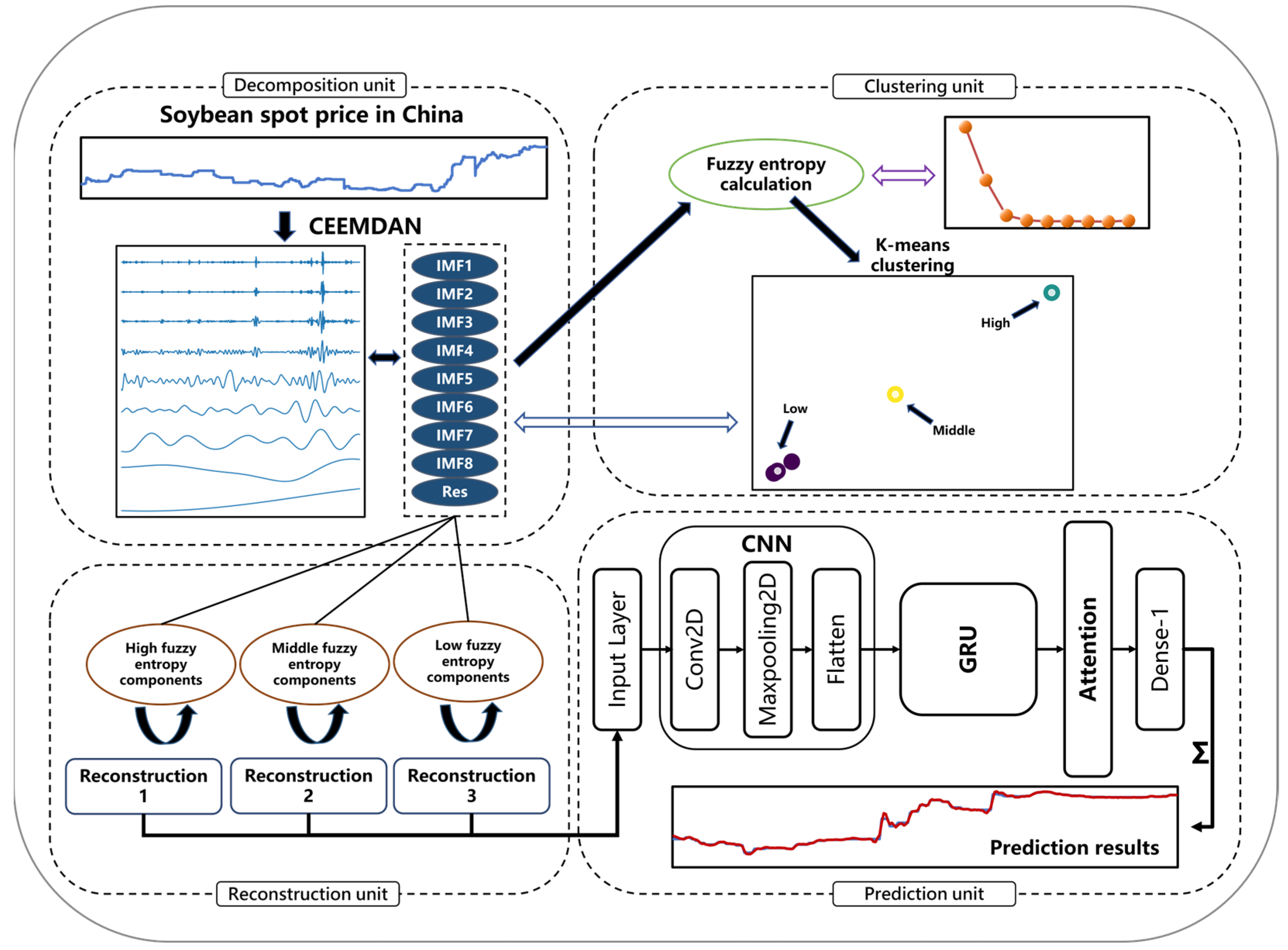
2.1. Overall Framework of the Mixed-Method Model

The proposed prediction model is based on the hybrid CNN-GRU deep learning technique and adds an attention mechanism to capture the characteristic messages and temporal relationships of the reconstructed components using the frequency decomposition algorithm CEEMDAN and K-means clustering with fuzzy entropy. This paper’s proposed model can be divided into two main sections.

The first is the decomposition part. Using the CEEMDAN approach, the original soybean price series is divided into components. Fuzzy entropy is calculated for each component to determine its level of complexity. The complexity components are then approximated using K-means clustering to produce labels for high, middle, and low fuzzy entropy. The process of component rebuilding follows. The second is the prediction part. The reconstructed components are predicted using a dual-coupled neural network (CNN-GRU) encapsulating the attention mechanism. To obtain the forecast findings, the final linear integration is carried out (see Figure 1).

The detailed modeling steps follow:

(1)

Soybean prices are decomposed by CEEMDAN into IMFs and Residual, which are then sorted from high to low frequencies;

(2)

K-means clustering is repeated for the decomposed components after the fuzzy entropy magnitude is calculated. An approximate component reconstruction is then performed;

(3)

Three types of reconstructed components are predicted by the CNN-GRU-Attention model, and then the outcomes are linearly integrated to get the final results.

2.2. CEEMDAN

Complete ensemble empirical mode decomposition with adaptive noise [48] (CEEMDAN) effectively eliminates the mode-mixing problem in empirical mode decomposition [49] (EMD). The reconstruction error is nearly zero compared to ensemble empirical mode decomposition [50] (EEMD), which drastically reduces the computational cost.

Define $E_n(·)$ as the modal component of the $n$th stage generated by applying the EMD algorithm, and the $n$th modal component generated by the CEEMDAN algorithm is denoted as an intrinsic mode function $IM{F}_n$. The implementation steps of the CEEMDAN method are as follows:

(1) The signal $x\left(t\right)$ to be decomposed is added to a Gaussian white noise sequence with $N$ times mean 0 to construct the sequence $x_i\left(t\right)\left(i=1,2,\cdots ,N\right)$.

$$\begin{array}{c}{x}_i\left(t\right)=x\left(t\right)+\epsilon {\delta }_i\left(t\right)\end{array}$$

(1)

where $\epsilon$ is the Gaussian white noise weight coefficient, ${\delta }_i\left(t\right)$ is the white noise sequence added for the $i$th time.

(2) Decompose $x_i\left(t\right)$ by applying the EMD algorithm to obtain the first modal component ($IMF$) and the first unique residual component $r_1\left(t\right)$.

$$IM{F}_1\left(t\right)=\frac{1}{N}{\displaystyle \sum }_{i=1}^{N}IM{F}_1^i\left(t\right)$$

(2)

$$\begin{array}{c}{r}_1\left(t\right)=x\left(t\right)-IM{F}_1\left(t\right)\end{array}$$

(3)

(3) Add noise to the residual component of the $j$th ($j=2,3,\cdots ,N$) stage after decomposition and continue to apply EMD for decomposition.

$$IM{F}_j\left(t\right)=\frac{1}{N}{\displaystyle \sum }_{i=1}^N{E}_1\left[r_{j-1}\left(t\right)+{\epsilon }_{j-1}{E}_{j-1}\left({\delta }_i\left(t\right)\right)\right]$$

(4)

$$\begin{array}{c}{r}_j\left(t\right)=r_{j-1}\left(t\right)-IM{F}_j\left(t\right)\end{array}$$

(5)

(4) Repeat step 3 until the termination condition is satisfied. The termination criterion is that the number of residual signal extremum points should be at most two. Finally, the original signal sequence is decomposed into $N$ modal components and the residual term $R\left(t\right)$.

$$x\left(t\right)={\displaystyle \sum }_{n=1}^{N}IM{F}_n\left(t\right)+R\left(t\right)$$

(6)

2.3. Fuzzy Entropy and K-Means Clustering

2.3.1. Fuzzy Entropy

Fuzzy Entropy [51] is a nonlinear dynamic indicator of time series complexity measure that uses an exponential function to fuzzy the similarity measure formula and make its value fluctuate continuously and smoothly with parameter changes.

(1) For a time series $\left\{\mathit{u}\left(i\right):1\le i\le N\right\}$ of a given length $N$, the vector set sequence $\{{\mathit{X}}_i^m,i=1,2,\dots ,N-m+1\}$ can be constructed by

$$\begin{array}{c}{\mathit{X}}_i^m=\left\{\mathit{u}\left(i\right),\mathit{u}\left(i+1\right),\dots ,\mathit{u}\left(i+m-1\right)\right\}-{\mathit{u}}_0\left(i\right)\end{array}$$

(7)

where $m$ is the embedding dimension and ${\mathit{u}}_0\left(i\right)$ is the baseline of ${\mathit{X}}_i^m$, defined by

$${\mathit{u}}_0\left(i\right)=\frac{1}{m}{\displaystyle \sum }_{j=0}^{m-1}\mathit{u}\left(i+j\right)$$

(8)

(2) The distance $d_{ij}^m$ between two vectors ${\mathit{X}}_i^m$ and ${\mathit{X}}_j^m$ is defined by

$$\begin{array}{c}{d}_{ij}^m=d\left[{\mathit{X}}_i^m,{\mathit{X}}_j^m\right]=\underset{k\in \left(0,m-1\right)}{\max }\left\{\left|\left[\mathit{u}\left(i+k\right)-{\mathit{u}}_0\left(i\right)\right]-\left[\mathit{u}\left(j+k\right)-{\mathit{u}}_0\left(j\right)\right]\right|\right\} \end{array}$$

(9)

where $1\le i,j\le N-m+1,i\ne j$.

(3) Based on the distance $d_{ij}^m$ defined above, the similarity of ${\mathit{X}}_i^m$ and ${\mathit{X}}_j^m$ can be calculated using the fuzzy function.

$$\begin{array}{c}{D}_{ij}^m=\mu \left(d_{ij}^m,n,r\right)={\mathrm{e}}^{-In2{\left(d_{ij}^m/r\right)}^n}\end{array}$$

(10)

$r$ is the similarity tolerance parameter.

(4) The matching template probability function ${\varphi }^m$ for $m$ is defined as follows:

$${\varphi }^m\left(n,r\right)=\frac{1}{N-m}{\displaystyle \sum }_{i=1}^{N-m}(\frac{1}{N-m-1}{\displaystyle \sum }_{j=1,j\ne i}^{N-m}{D}_{ij}^m)$$

(11)

(5) Similarly, repeating steps 1 to 4 for $m+1$, the following equation for ${\varphi }^{m+1}\left(n,r\right)$ can be obtained.

$${\varphi }^{m+1}\left(n,r\right)=\frac{1}{N-m}{\displaystyle \sum }_{i=1}^{N-m}(\frac{1}{N-m-1}{\displaystyle \sum }_{j=1,j\ne i}^{N-m}{D}_{ij}^{m+1})$$

(12)

(6) The formula for the fuzzy entropy value of the initial time series $\left\{\mathit{u}\left(i\right):1\le \mathrm{i}\le N\right\}$ is defined as follows:

$$\begin{array}{c}Fu\mathit{z}\mathit{z}yEn\left(m,n,r\right)=\underset{N\to \infty }{\lim }[\ln {\varphi }^m\left(n,r\right)-\ln {\varphi }^{m+1}\left(n,r\right)]\end{array}$$

(13)

2.3.2. K-Means Clustering

K-means clustering [52] is an unsupervised algorithm that is widely used and is scalable and efficient for fitting datasets, aiming to classify object $\mathit{X}\left(t\right)=\left\{x_1\left(t\right),x_2\left(t\right),\cdots ,x_n\left(t\right)\right\}$ into the $K$ clusters with the closest mean. The $K$ cluster center of mass is calculated starting with the input of the cluster.

(1) Calculate the distance between the data points ${\mathit{X}}^k\left(t\right)=\left\{x_1^k\left(t\right),x_2^k\left(t\right),\cdots ,x_{nk}^k\left(t\right)\right\}$ and the $K$ cluster centers, connecting each point to the nearest center.

$$c^k\left(t\right)=\frac{1}{n_k}{\displaystyle \sum }_{i=1}^{n_k}{x}_i^k\left(t\right)$$

(14)

(2) Repeat the calculation of the $K$ center of mass position until it no longer moves, thus grouping the objects with $\underset{x_i^k\in X}{\min }J\left(t\right)$ at their minimization.

$$J\left(t\right)={\displaystyle \sum }_{k=1}^K{\displaystyle \sum }_{i=1}^n\left||x_i^k\left(t\right)-c^k\left(t\right)|\right|$$

(15)

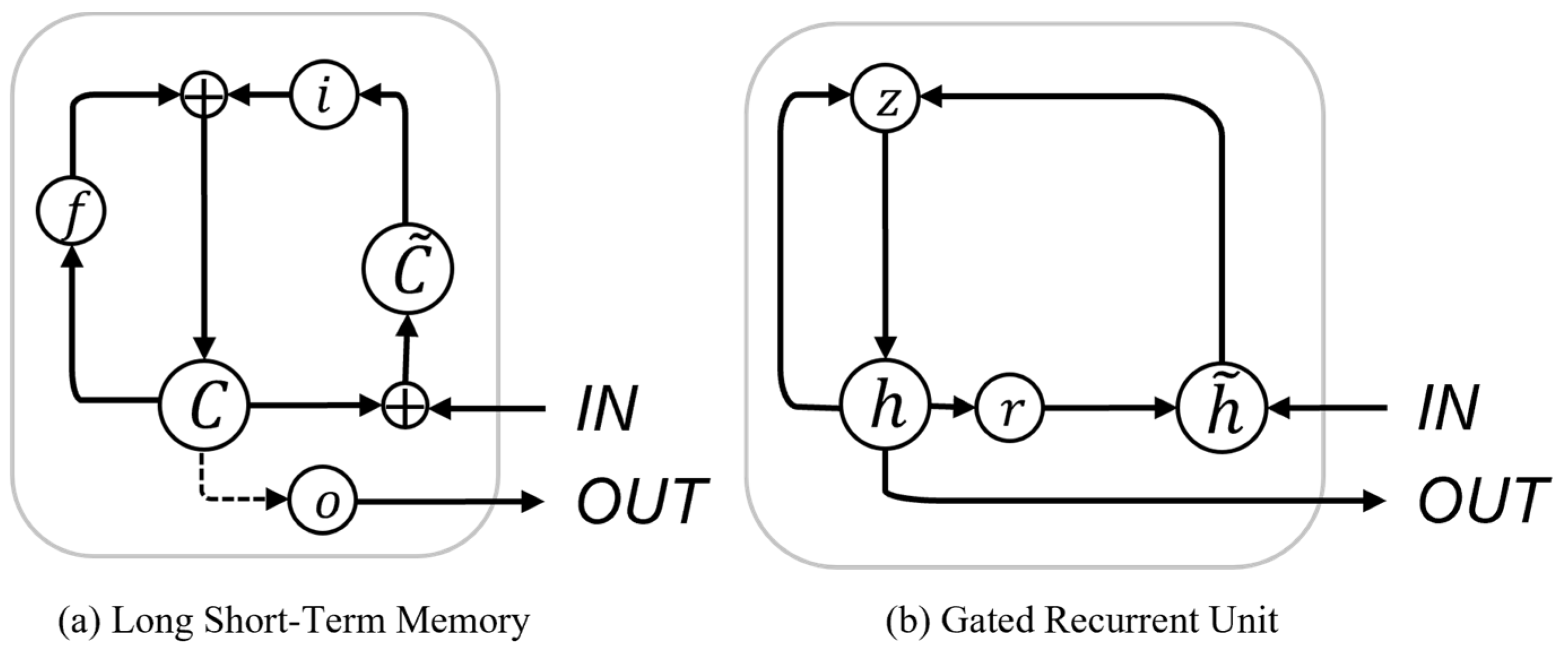
2.4. Description of CNN-GRU-Attention

2.4.1. CNN

Convolutional neural network [53] (CNN) performs layer-by-layer convolution and pooling operations on the input data. The convolution layer is the core of CNN, which performs the convolution operation on the input using local connectivity and weight sharing to extract the deep features. The convolution process can be represented by the following equation:

$$\begin{array}{c}\mathit{C}=f\left(\mathit{X}·\mathit{W}+\mathit{b}\right)\end{array}$$

(16)

$\mathit{C}$ is the output feature map of the convolution layer, $\mathit{X}$ is the input data, $f(·)$ is the nonlinear activation function, $\mathit{W}$ is the weight vector of the convolution kernel, $\mathit{b}$ is the bias term.

The pooling layer performs operations on the output of the convolutional layer through certain rules to retain the main features while reducing the number of parameters and computation to prevent overfitting. The pooling process can be expressed by the following equation:

$$\begin{array}{c}\mathit{p}=pool\left(\mathit{C}\right)\end{array}$$

(17)

2.4.2. GRU

A Gated recurrent unit [54] (GRU) is a modified version of the long short-term memory (LSTM) architecture that combines the input gate and forget gate into an update gate with an additional reset gate (see Figure 2).

The GRU model can regulate the information without storing the cell. At time $t$, the activation function ${\mathit{h}}_t^j$ is a linear interpolation between the candidate activation function ${\mathit{h}}_t^{\sim j}$ and the previous activation function ${\mathit{h}}_{t-1}^j$.

$$\begin{array}{c}{\mathit{h}}_t^j=\left(1-{\mathit{z}}_t^j\right){\mathit{h}}_{t-1}^j+{\mathit{z}}_t^j{\mathit{h}}_t^{\sim j}\end{array}$$

(18)

The update gate ${\mathit{z}}_t^j$ determines the degree of cell update activation. The activation function is ${\mathit{h}}_t^{\sim j}$:

$$\begin{array}{c}{\mathit{z}}_t^j=\sigma {\left({\omega }_z{\mathit{A}}_t+U_t{\mathit{h}}_{t-1}\right)}^j\end{array}$$

(19)

$$\begin{array}{c}{\mathit{h}}_t^{\sim j}=tanh{\left(\omega {\mathit{A}}_t+U_r\left({\mathit{r}}_t^j\times {\mathit{h}}_{t-1}\right)\right)}^j\end{array}$$

(20)

${\mathit{r}}_t^j$ is the reset gate, which is closed to allow the unit to forget past information.

$$\begin{array}{c}{\mathit{r}}_t^j=\sigma {\left({\omega }_r{\mathit{A}}_t+{\mathit{h}}_{t-1}\right)}^j\end{array}$$

(21)

$\sigma$ is the sigmoid function, $\omega$ is the weight or parameter. The update gate controls the past state, cells with long-term relevance are called active update gates $z$, and cells with short-term relevance are called active reset gates $r$.

2.4.3. Attention Mechanism

The concept of an attention mechanism [55] can be explained as carefully selecting important items from a large amount of information and concentrating on those elements while disregarding the majority of the irrelevant information. The process of focusing is reflected in the weight coefficient calculation, where a higher weight denotes paying more attention.

The model computes the environment vector ${\mathit{c}}_i$ based on the input vector ${\mathit{h}}_i\left(i=1,2,\cdots ,k\right)$ and jointly predicts the current hidden state. ${\mathit{c}}_i$ can be obtained from a weighted average of the previous states.

$${\mathit{c}}_i={\displaystyle \sum }_{i=1}^k{a}_i{\mathit{h}}_i$$

(22)

The attention weight $a_i$ is obtained by calculating the score $s_i$, according to which the degree of influence of each hidden layer vector on the output is evaluated.

$$\begin{array}{c}{s}_i=\tanh \left(w^T+{\mathit{b}}_i\right)\end{array}$$

(23)

The correlation degree of $h_i$ and $c_i$ is represented by $s_i$. The final weight coefficients are acquired by normalizing $s_i$ using the SoftMax function.

$$a_i=softmax\left(s_i\right)=\frac{e^{s_i}}{{\sum }^{ }j{e}^{s_j}}$$

(24)

3. Analysis of Experiments

The purpose of this research is to implement the CEEMDAN method with fuzzy entropy K-means clustering of components and CNN-GRU-Attention hybrid model to predict soybean prices. The model was split into two parts: the decomposition part (CEEMDAN with component clustering) and the prediction part (CNN-GRU-Attention). The entire empirical analysis is centered on major focused issues.

First, how effective is the model’s prediction compared to other approaches? Does CNN-GRU-Attention consistently predict soybean prices with high accuracy? Second, consider whether the decomposition was more useful than the alternative that wasn’t used. Third, is the suggested model decomposition approach better than alternative decomposition techniques? Are the overall outcomes of the suggested model optimal for predicting soybean prices? Before discussing the specific model, we will describe the data and criteria used in the empirical evidence.

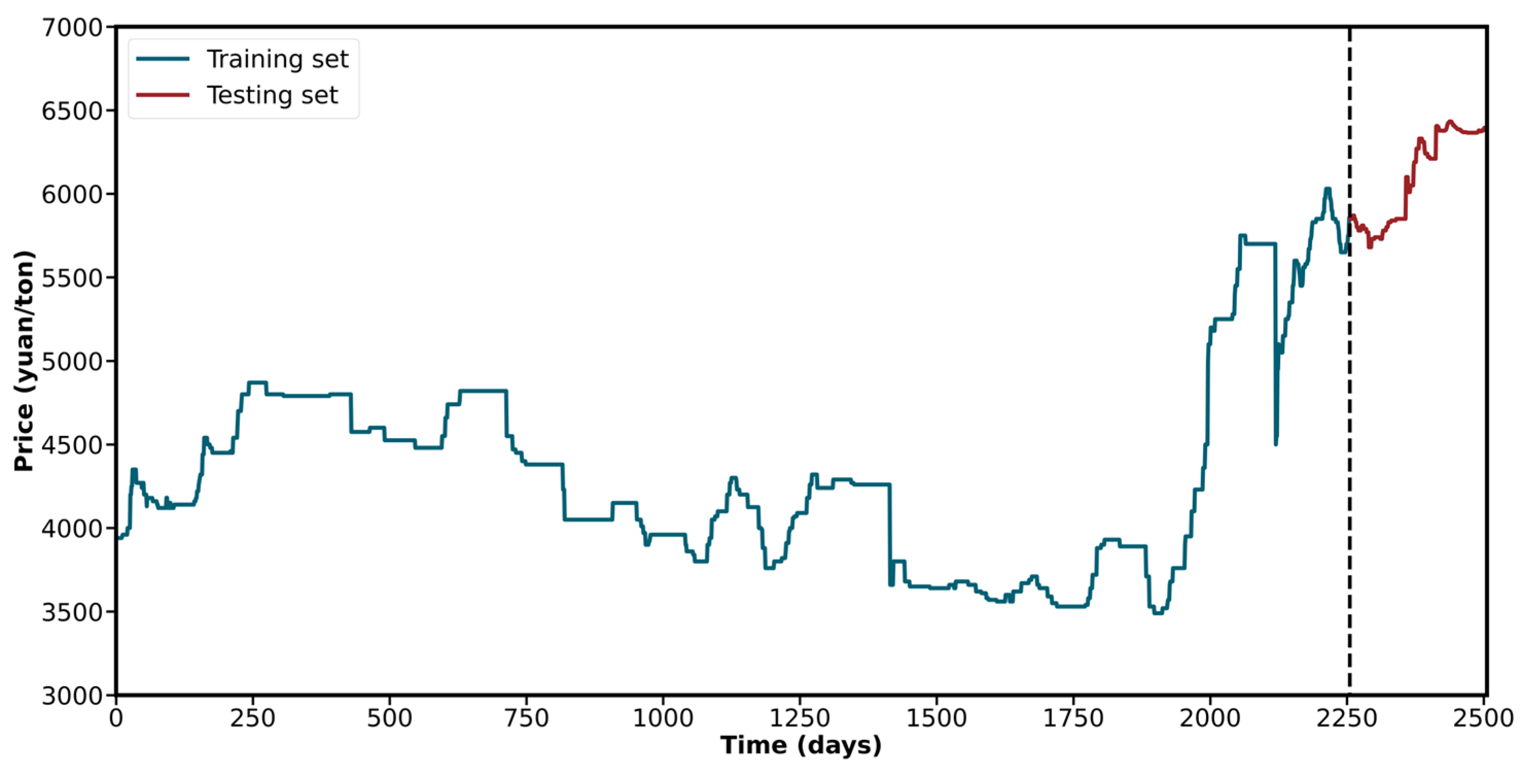
3.1. Data Sources and Standard Measurement

In this paper, China’s soybean spot price time series data is selected as model inputs and forecast objects. The data are obtained from the Eastmoney Choice financial database (https://choice.eastmoney.com/ (accessed on 29 May 2022)). The data frequency is daily, and the price unit is “yuan/ton”. The timespan runs from 29 July 2011 to 27 May 2022, with 2505 sample data. The first 90 percent is the training set, and the last 10 percent is the test set. The data is described in

Table 1. Basic statistical analysis of soybean spot prices.

Object	Count	Mean	Min	Max	Standard Deviation
Soybean	2505	4499.3869	3490.0000	6433.5400	779.6956
Training set	2255	4321.7175	3490.0000	6030.0000	592.3186
Testing set	250	6101.9643	5680.0000	6433.5400	270.3752

, and the graphical description is shown in Figure 3.

The series is Min-Max normalized prior to entering the prediction phase of the model training, and the processing formula is $x^{\prime }=\left(x-x_{min}\right)/\left(x_{max}-x_{min}\right)$ where $x$ and $x^{\prime }$ represent the original and normalized data, respectively.

The difference between the observed and predicted values—known as the loss error—is used to assess the effectiveness of model prediction. The evaluation criteria employed in this research are root mean square error (RMSE), mean absolute percentage error (MAPE), and mean absolute error (MAE). The formulas for their calculations are as follows, accordingly.

$$RMSE=\sqrt{\frac{1}{n}{\displaystyle \sum }_{i=1}^n{\left({\widehat{y}}_i-y_i\right)}^2}$$

(25)

$$MAPE=\frac{100\%}{n}{\displaystyle \sum }_{i=1}^n\frac{|{\widehat{y}}_i-y_i|}{y_i}$$

(26)

$$MAE=\frac{1}{n}{\displaystyle \sum }_{i=1}^n|{\widehat{y}}_i-y_i|$$

(27)

$n$ is the length of the test set sequence, $y_i$ and ${\widehat{y}}_i$ is the true value and the predicted value, respectively. $i$ is the test set sequence number. Obviously, the smaller the value of the evaluation criteria in the (0, +∞) range, the more reliable and accurate the prediction results.

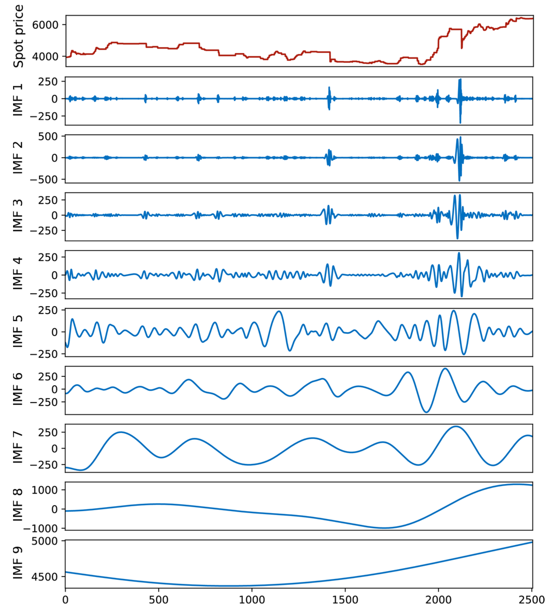
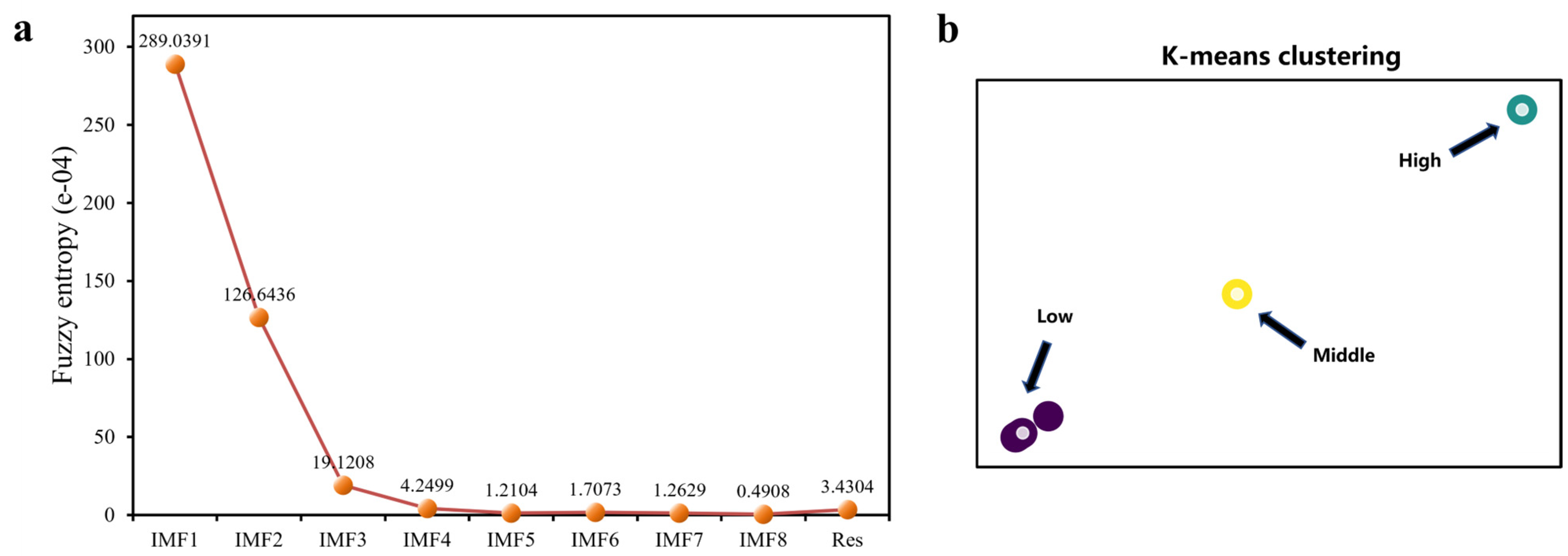
3.2. CEEMDAN Processing

The data are divided up into numerous kinds of spectra by the frequency decomposition algorithm. The spot price of soybeans is divided into 8 IMFs and 1 residual using CEEMDAN. The components are arranged from high to low frequency, as shown in Figure 4.

3.3. Fuzzy Entropy-Based Components Clustering

Fuzzy entropy calculation and K-means clustering were performed following the decomposition of the price series into reciprocal spectra. The results are shown in Figure 5. Furthermore, in

Table 2. The clustering labels of different decomposed components.

IMF1	IMF2	IMF3	IMF4	IMF5	IMF6	IMF7	IMF8	Res
H1	M1	L1	L2	L3	L4	L5	L6	L7

Notes: H, M, and L represent high, middle, and low fuzzy entropy clustering labels, respectively.

, the high and middle fuzzy entropy components, H1 and M1, respectively, are represented. The low fuzzy entropy components are designated by L1–L7. The clustering explains how different sequence information is incorporated into various components.

Next, L1–L7 are reconstructed into new components to prepare the prediction. H1 and M1 do not need to be reconstructed because they are already separate components.

3.4. Model Instructions and Parameter Setting

The accuracy of the results in the prediction phase was impacted by using different time steps. Because of the small size and lack of global parameters when the time step is 3, the prediction results exhibit substantial variances and some data oscillations. When the time step is 30, the time horizon is too wide, and it is easy to overlook some defining characteristics in the short term, which produces unreliable prediction outcomes. The final time step is chosen as 10 since it has the lowest error and maximum accuracy.

A total of 18 models were used for comparison in the prediction analysis, and the specific abbreviations and instructions are shown in

Table 3. The instructions for comparison models.

Model	Model Instruction	Abbreviation
Model 1	Convolutional Neural Network	CNN
Model 2	Combined model of Convolutional Neural Network and Gated Recurrent Unit	CNN-GRU
Model 3	Combined model of Convolutional Neural Network and Gated Recurrent Unit with Attention mechanism	CNN-GRU-Attention
Model 4	Gated Recurrent Unit	GRU
Model 5	Gated Recurrent Unit with Attention mechanism	GRU-Attention
Model 6	Long Short-term Memory network	LSTM
Model 7	Multilayer Perceptron model	MLP
Model 8	Support Vector Regression model	SVR
Model 9	A hybrid model by integrating CEEMDAN with fuzzy entropy clustering and CNN	CEEMDAN-CNN
Model 10	A hybrid model by integrating CEEMDAN with fuzzy entropy clustering and CNN-GRU	CEEMDAN-CNN-GRU
Model 11 (Proposed model)	A hybrid model by integrating CEEMDAN with fuzzy entropy clustering and CNN-GRU with Attention mechanism	CEEMDAN-CNN-GRU-Attention
Model 12	A hybrid model by integrating CEEMDAN with fuzzy entropy clustering and GRU	CEEMDAN-GRU
Model 13	A hybrid model by integrating CEEMDAN with fuzzy entropy clustering and GRU with Attention mechanism	CEEMDAN-GRU-Attention
Model 14	A hybrid model by integrating CEEMDAN with fuzzy entropy clustering and LSTM	CEEMDAN-LSTM
Model 15	A hybrid model by integrating CEEMDAN with fuzzy entropy clustering and MLP	CEEMDAN-MLP
Model 16	A hybrid model by integrating CEEMDAN with fuzzy entropy clustering and SVR	CEEMDAN-SVR
Model 17	A hybrid model by integrating EMD with fuzzy entropy clustering and CNN-GRU with Attention mechanism	EMD-CNN-GRU-Attention
Model 18	A hybrid model by integrating EEMD with fuzzy entropy clustering and CNN-GRU with Attention mechanism	EEMD-CNN-GRU-Attention

. In addition, the hyperparameters of the main deep learning models (CNN and GRU) used in the proposed model are described in

Table 4. Parameter setting of the hybrid proposed model.

Models	Parameters	Values
CNN	Filters	64
	Kernel size	2
	Activation	Relu
	Pooling size	2
	Flatten	-
	Epochs	500
	Batch size	64
GRU	Neurons	128
	Activation	tanh
	Epochs	500
	Batch size	64
Attention	Weights compute	Softmax

.

3.5. Prediction Results

The experiment was split into two main sections to address the three key difficulties stated at the start of the empirical analysis. The first compares the prediction part model’s (CNN-GRU-Attention) results to examine whether it can accurately and consistently forecast soybean prices. The second is a comparison of the predictions made using the various models that have been suggested to see if using the decomposition method increases the precision of the prediction part. To confirm the best option, further evaluate the predictions from various decomposition methods.

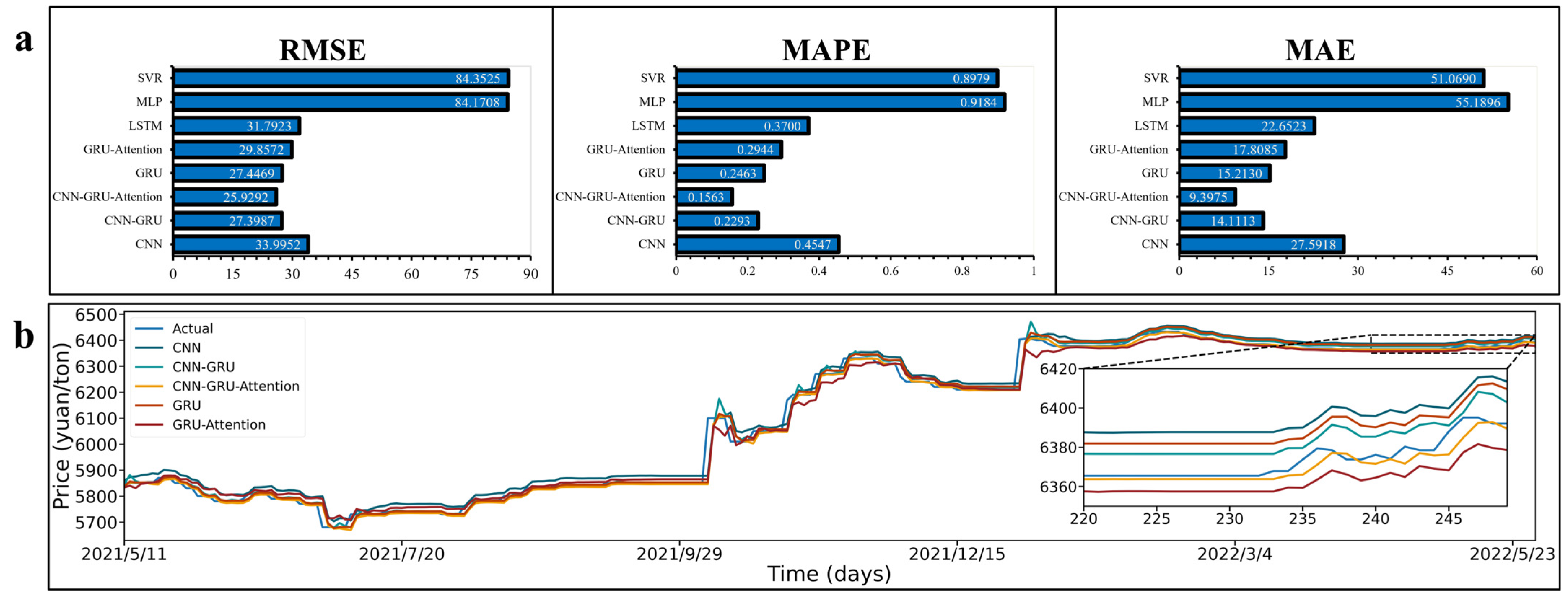
3.5.1. Comparison of the Prediction Part

The prediction part (CNN-GRU-Attention) is compared with widely used deep learning and machine learning methods based on the same data and parameters before utilizing the total suggested model. The specific prediction results are shown in Figure 6.

A calculation was utilized to determine the percentage decrease in the particular evaluation criteria of the comparison models to have a clearer representation of how much the prediction accuracy of one model improved over another (e.g., the Percentage change in RMSE value regarding the comparison of CNN-GRU and CNN-GRU-Attention = 100% × (CNN-GRU-CNN-GRU-Attention)/CNN-GRU).

As shown in Figure 6, the RMSE, MAPE, and MAE values for CNN-GRU are 27.3987, 0.2293, and 14.1113, respectively. For CNN-GRU-Attention, the values are 25.9292, 0.1563, and 9.3975. Compared to the CNN-GRU without the attention mechanism, the CNN-GRU-Attention model reduced the RMSE, MAPE, and MAE values by 5.36%, 31.84%, and 33.40%, respectively. It shows that the attention mechanism has a highly developed capacity for information extraction and that, when given weights to increase prediction accuracy, it could efficiently extract the information relations handled by the previous model. The inclusion of the attention mechanism makes it possible to more accurately identify several significant trends and recurrent characteristics within the soybean price series, which frequently indicate some issue or phenomenon inside the spot market.

In contrast to the CNN (RMSE: 33.9952, MAPE: 0.4547, and MAE: 27.5918) or GRU (27.4469, 0.2463, and 15.2130) models alone, the CNN-GRU model has RMSE values that are 19.40% and 0.18% lower, MAPE values that are 49.57% and 45.83% lower, and MAE values that are 48.86% and 44.86% lower. The value of information processing may be understood by focusing on how CNN dominated data characteristic recognition and GRU-anchored chronological information prediction, improving combined prediction accuracy significantly. The combination of the two models outlined above is thus a more crucial step in the prediction of soybean prices. The profound potential relationship between input feature space and temporal dependencies is the baseline for the model to achieve the benefits.

In addition, the GRU-Attention model performs slightly worse than GRU, likely because it solely considers chronological correlation. This causes the model’s accuracy to decline since the attention mechanism unintentionally increases the weight of unimportant information.

After linking the attention mechanism, the prediction part model’s capacity to discern the depth of the input feature space and chronological correlation is confirmed, giving it a significant advantage in soybean spot price prediction.

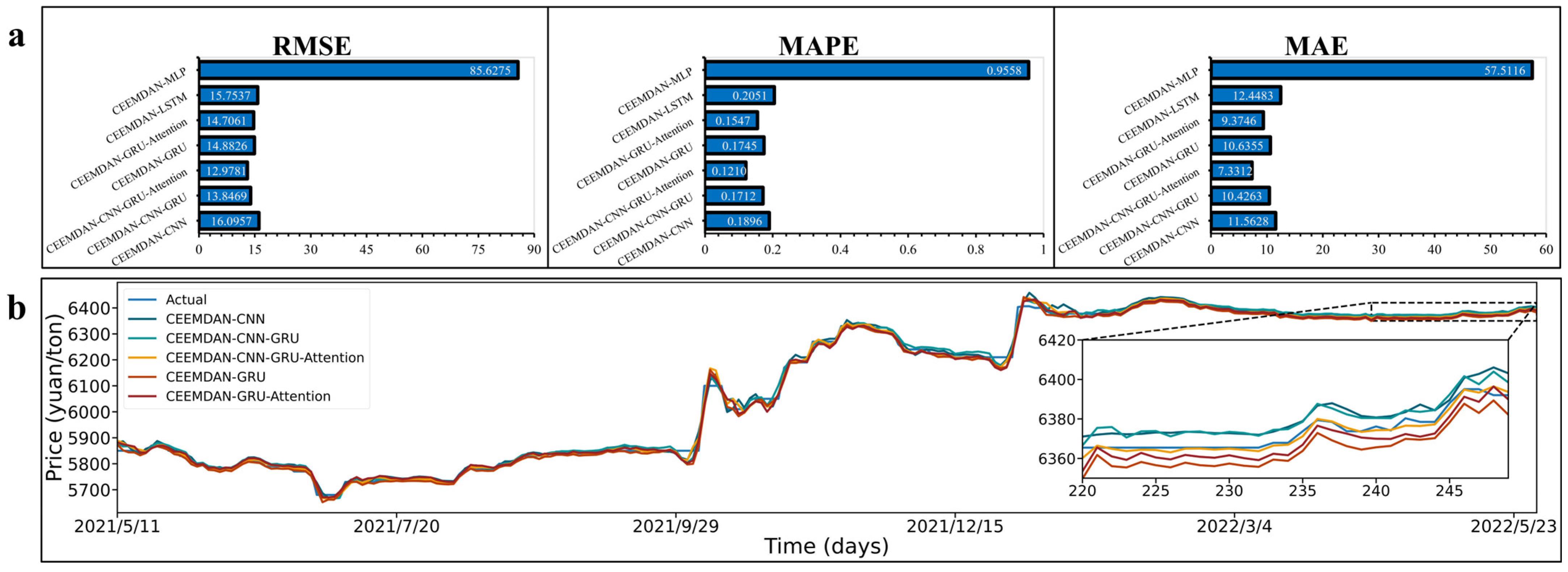
3.5.2. Comparison of the Hybrid Models

Validation was conducted following the implementation of the decomposition part using the same parameters and data set. The predictions for their standard measurement are shown in Figure 7. In addition, the RMSE, MAPE, and MAE values for CEEMDAN-SVR, which are 334.7073, 4.7625, and 280.0073, respectively, are not represented in the figure due to the anomalous values.

As seen in Figure 7, the value of each evaluation criterion gradually declines as the prediction model’s complexity rises after assembling the decomposition part. It can be inferred that suitable stripping disassembled the data information with good sequence complexity gradient and expected partial model applicability enhancement after CEEMDAN processing and reconstructing the components by fuzzy entropy clustering.

In terms of RMSE, MAPE, and MAE, CEEMDAN-CNN-GRU has values of 13.8469, 0.1712, and 10.4263. The results for CEEMDAN-GRU-Attention are 14.7061, 0.1547, and 9.3746, correspondingly. When compared to the CEEMDAN-CNN-GRU and CEEMDAN-GRU-Attention models, the RMSE values of CEEMDAN-CNN-GRU-Attention (12.9781) are decreased by 6.27% and 11.75%, the MAPE values (0.1210) are decreased by 29.32% and 21.78%, and the MAE values (7.3312) are decreased by 29.69% and 21.80%, respectively. This indicates that the prediction component is still applicable in component prediction, which lowers the sequence’s overall complexity and improves the model’s ability to understand distinctive data and temporal relevance to produce better outcomes.

Meanwhile, CEEMDAN-CNN-GRU has 13.97% and 6.96% lower RMSE, 9.70% and 1.89% lower MAPE, 9.82%, and 1.97% lower MAE values than CEEMDAN-CNN (RMSE: 16.0957, MAPE: 0.1896 and MAE: 11.5628) and CEEMDAN-GRU (RMSE: 14.8826, MAPE: 0.1745 and MAE: 10.6355), respectively. It is verified that the joint model has the same good prediction performance after decomposition as the individual model.

Moreover, as illustrated in Figure 8, it is clear that the implementation of the decomposition part significantly improves overall prediction accuracy. The result of CEEMDAN-CNN-GRU-Attention has RMSE, MAPE, and MAE values of 49.95%, 22.58%, and 21.99% lower than CNN-GRU-Attention, respectively. The evaluation metrics decrease significantly compared to the prediction part models with proposed model components, demonstrating the effectiveness in raising applicability and utility.

The value information contained in the series is effectively rearranged following the series decomposition–component clustering procedure, making it more appropriate for the combination model’s forecasting component. The aforementioned findings further show that, to improve forecasting outcomes, the complex combination model for soybean spot prices can more fully and successfully account for both short-term repetitious information and long-term reliance in its series.

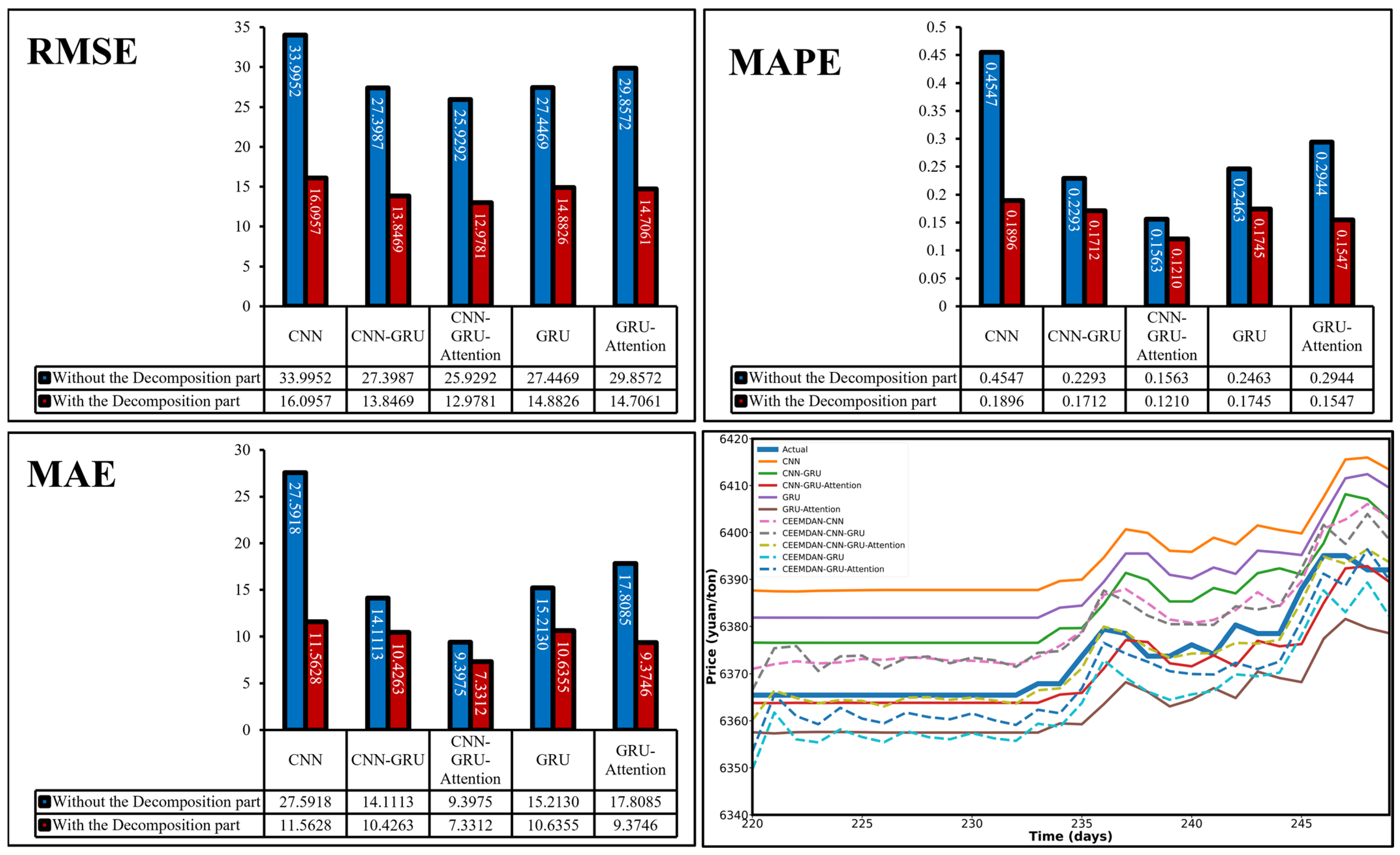
3.5.3. Comparison of Various Decomposition Methods

The prediction results of the standard measurement caused by different decomposition means are depicted in Figure 9, which are also tested using the same data set and parameter expansion.

As demonstrated in Figure 9, EMD-CNN-GRU-Attention has the following RMSE, MAPE, and MAE values: 21.6874, 0.1988, and 12.0041, respectively. The respective values for EEMD-CNN-GRU-Attention are 23.6603, 0.2999, and 18.1278. The prediction part with CEEMDAN as the axis produces the best training results with 40.16% and 45.15% lower RMSE values, 39.13% and 59.65% lower MAPE values, 38.93%, and 59.56% lower MAE values than EMD and EEMD, respectively. It proves that the CEEMDAN-CNN-GRU-Attention has superior model stability, fits a stronger trend of data variance, and has greater consistency of evaluation criteria. The relative advantages of making improvements are becoming more and more clear.

As seen above, the CEEMDAN technique is more suited to deconstructing the various hidden implicit information about soybean prices. The serial complexity of soybean prices, however, dictates the limitations of its application, despite the partial performance increase of the EMD method. In addition, the EEMD processing’s overall assessment metrics are slightly greater than those of the EMD, most likely due to its inability to completely remove Gaussian white noise during reconstruction or prediction, which is overdone in terms of processing.

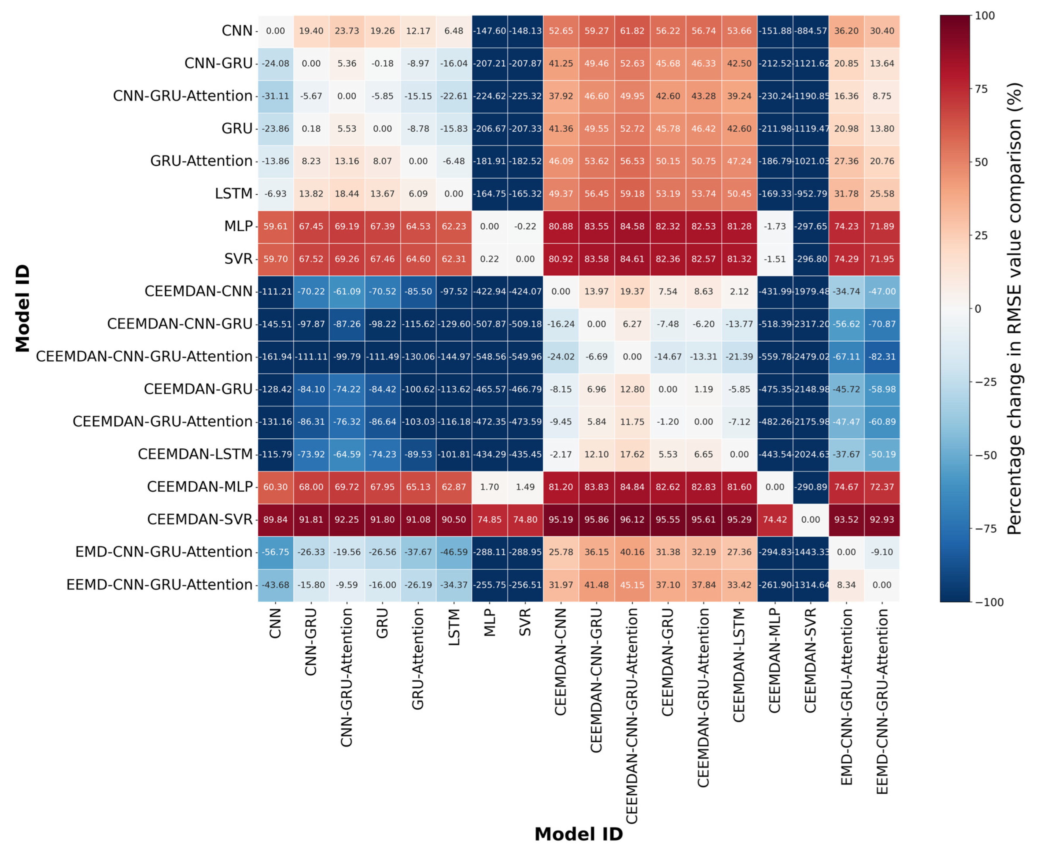
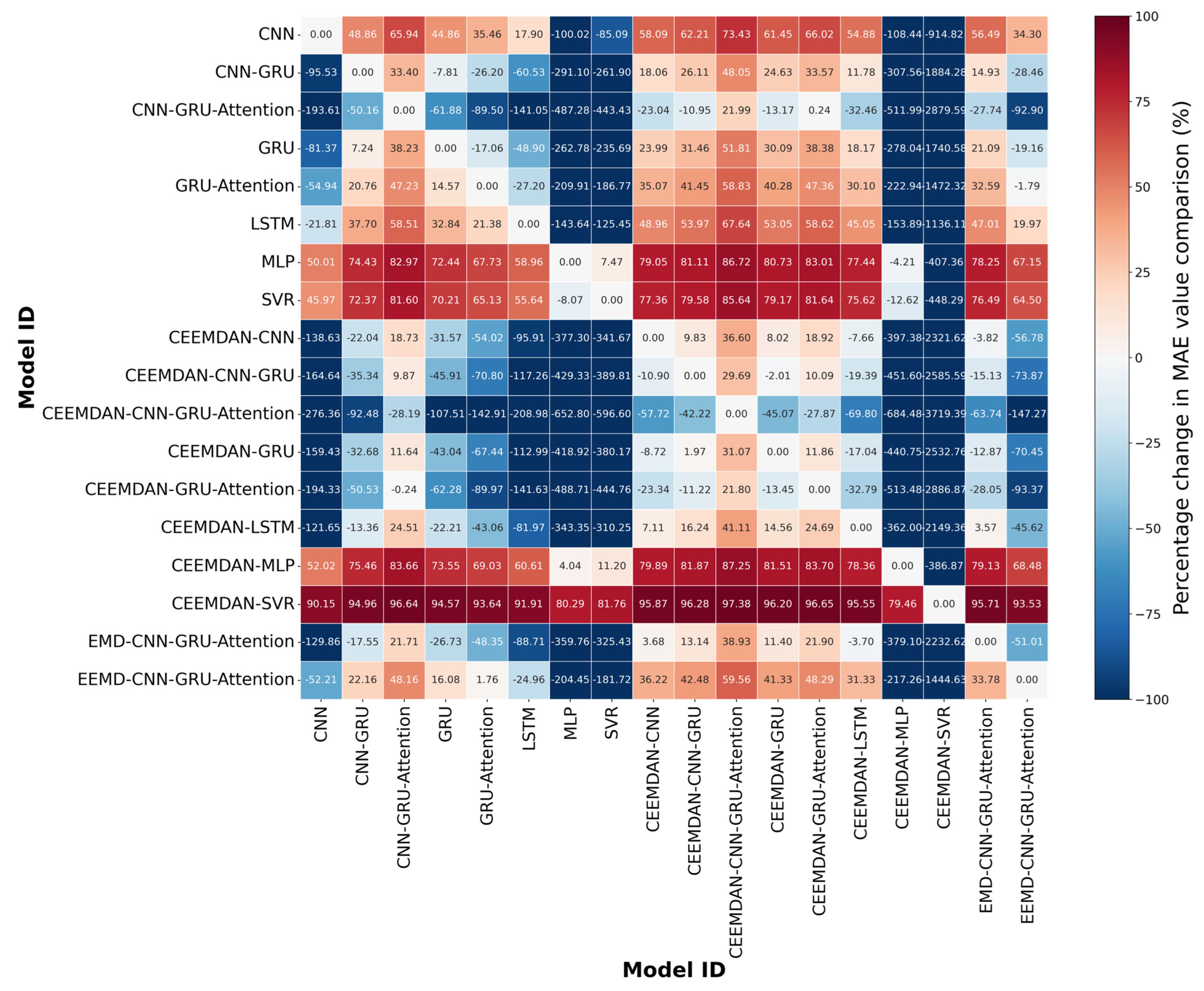
3.5.4. The Comparison of All Model Components

The one-by-one comparison results of the models involved in the research are illustrated in Figure 10, Figure 11 and Figure 12 to display how the RMSE, MAPE, and MAE values have increased or decreased relative to each other. The purpose of the comparison is to determine the percentage change in prediction accuracy between any two models compared to the particular value of the evaluation standards. When the percentage change is negative (positive), it indicates a percent reduction (rise) in the specific value of the evaluation criterion for the model in the row compared to the model in the column or a percent improvement (decrease) in the model’s ability to predict outcomes accurately. Utilizing color is a more perceptual technique to see the shift. The prediction accuracy of the model in the row over the model in the column is higher when the blue degree of the color block between the two models is darker, whereas a lower prediction performance is indicated by a deeper red degree. For instance, in Figure 10, the RMSE value of CNN-GRU-Attention is 49.95% higher than that of CEEMDAN-CNN-GRU-Attention and 31.11% lower than that of the CNN model alone, implying that the model prediction accuracy of CNN-GRU-Attention is less than the former and greater than the latter. Accordingly, the three models with the decreasing order prediction accuracy for the data are CEEMDAN-CNN-GRU-Attention, CNN-GRU-Attention, and CNN. All three assessment criteria show a huge decrease when the decomposition part is combined compared to the prediction part alone, and some findings are even close to double the improvement.

After adaptive decomposition, the fuzzy entropy clustering strategy can efficiently mine the complexity and difference patterns of component information. This method also improves the model’s adaptability and functionality while increasing the performance level of the sequence input characteristic space and chronological dependence correlations. Also, the CNN-GRU-Attention model has much higher prediction accuracy than all other models in its prediction part. In all compared instances, the model with the decomposition part outperforms the model without, in terms of prediction accuracy. Compared to previous strategies, the decomposition strategy suggested in this research offers the best model utility enhancement. In addition, the Supplementary Materials contain all the model predictions and the original data used in this research.

4. Conclusions and Discussion

In this paper, a decomposition-integration prediction model is proposed that combines a component clustering strategy with a dual-coupled neural network that incorporates an attention mechanism. The original sequence is processed by CEEMDAN using fuzzy entropy as a condition for K-means clustering of discrepant components. The reconstructed sequences are put into a CNN-GRU model for prediction, which integrates an attention mechanism.

Firstly, the integrated CNN-GRU model can effectively distill the data characteristics and temporal dependencies. The coupled attention mechanism achieves the input feature space and chronological importance assessment through the dynamic assignment of weights to deeply improve the prediction part. This is in line with the argument by Ribeiro and Coelho [56], which shows that the integrated models collectively forecast soybean prices more accurately than a single model.

Secondly, the complexity and volatility of time series can be decreased by using CEEMDAN. The results of the fuzzy entropy-based K-means clustering can efficiently combine the component information, greatly reduce the number of prediction models needed after adaptive decomposition, and improve adaptability and superiority. This is comparable to the findings of Wang et al. [43], who used the futures prices of wheat, corn, and soybeans for forecasting and showed that all hybrid models, when combined with the decomposition technique, outperformed the individually upgraded models.

Thirdly, two experimental sections are set up to address the three main issues brought up at the start of the empirical analysis. These sections comprehensively confirm that the proposed model can not only efficiently extract crucial characteristic information and recognize relative dependencies between long- and short-term time series but also improve prediction findings. The model parameters employed in the prediction part are predetermined. However, the idea put out by Xu and Zhang [8] can be a starting point for more research by examining various model settings for an algorithm, delay, hidden neuron, and data-splitting ratio.

Therefore, this research confirms that the fuzzy entropy K-means clustering, coupled with the attention neural network (CNN-GRU-Attention) and the application of the CEEMDAN approach, outperforms all models in the experiment and can more accurately predict China’s soybean spot price. In addition, Multiple uncertainties, including those related to climate change, natural disasters, international commerce, and macroeconomic policies, also impact soybean spot prices. Events with high stochasticity pose numerous difficulties for the soybean trade. To support the decomposition algorithm, this paper conducts research from a univariate time-series forecasting perspective. By considering different uncertainty characteristics and indirectly impacting statistical parameters [57], further study on the consequences of soybean price volatility and other studies can be done. Pre-processing elements like data complementation or cleaning can be considered, given the high complexity of nonlinearity and non-stationarity of soybean price series. The approaches utilized in this research all use pre-existing model frameworks. It is then possible to try to construct model methods for certain difficulties to offer suggestions for other similar prediction issues [58].

References

1. Yao, H.; Zuo, X.; Zuo, D.; Lin, H.; Huang, X.; Zang, C. Study on soybean potential productivity and food security in China under the influence of COVID-19 outbreak. Geogr. Sustain. 2020, 1, 163–171. [Google Scholar] [CrossRef]
2. Mallory, M.L. Impact of COVID-19 on medium-term export prospects for soybeans, corn, beef, pork, and poultry. Appl. Econ. Perspect. Policy 2021, 43, 292–303. [Google Scholar] [CrossRef] [PubMed]
3. Yu, X.; Liu, C.; Wang, H.; Feil, J.-H. The impact of COVID-19 on food prices in China: Evidence of four major food products from Beijing, Shandong and Hubei Provinces. China Agric. Econ. Rev. 2020, 12, 445–458. [Google Scholar] [CrossRef]
4. Kumar, A.; Pinto, P.; Hawaldar, I.T.; Spulbar, C.M.; Birau, F.R. Crude oil futures to manage the price risk of natural rubber: Empirical evidence from India. Agric. Econ. 2021, 67, 423–434. [Google Scholar] [CrossRef]
5. Panagiotou, D.; Tseriki, A. Directional predictability between trading volume and price returns in the agricultural futures markets: Risk implications for traders. J. Risk Financ. 2022, 23, 264–288. [Google Scholar] [CrossRef]
6. Salisu, A.A.; Vo, X.V.; Lawal, A. Hedging oil price risk with gold during COVID-19 pandemic. Resour. Policy 2020, 70, 101897. [Google Scholar] [CrossRef]
7. Goodwin, B.K.; Schnepf, R.; Dohlman, E. Modelling soybean prices in a changing policy environment. Appl. Econ. 2005, 37, 253–263. [Google Scholar] [CrossRef]
8. Xu, X.; Zhang, Y. Commodity price forecasting via neural networks for coffee, corn, cotton, oats, soybeans, soybean oil, sugar, and wheat. Intell. Syst. Account. Financ. Manag. 2022, 29, 169–181. [Google Scholar] [CrossRef]
9. Darroch, M.A.; Akridge, J.T.; Boehlje, M.D. Capturing value in the supply chain: The case of high oleic acid soybeans. Int. Food Agribus. Manag. Rev. 2002, 5, 87–103. [Google Scholar] [CrossRef]
10. Jia, F.; Peng, S.; Green, J.; Koh, L.; Chen, X. Soybean supply chain management and sustainability: A systematic literature review. J. Clean. Prod. 2020, 255, 120254. [Google Scholar] [CrossRef]
11. Richter, M.C.; Sørensen, C. Stochastic volatility and seasonality in commodity futures and options: The case of soybeans. SSRN 2002, 45, 301994. [Google Scholar] [CrossRef] [Green Version]
12. Ahumada, H.; Cornejo, M. Forecasting food prices: The case of corn, soybeans and wheat. Int. J. Forecast. 2016, 32, 838–848. [Google Scholar] [CrossRef]
13. Wu, L.; Liu, S.; Yang, Y. Grey double exponential smoothing model and its application on pig price forecasting in China. Appl. Soft Comput. 2016, 39, 117–123. [Google Scholar] [CrossRef] [Green Version]
14. Yu, Z.; Qin, L.; Chen, Y.; Parmar, M. Stock price forecasting based on LLE-BP neural network model. Phys. A Stat. Mech. Appl. 2020, 553, 124197. [Google Scholar] [CrossRef]
15. Wu, Y.-X.; Wu, Q.-B.; Zhu, J.-Q. Improved EEMD-based crude oil price forecasting using LSTM networks. Phys. A Stat. Mech. Appl. 2019, 516, 114–124. [Google Scholar] [CrossRef]
16. Yu, L.; Zhao, Y.; Tang, L. A compressed sensing based AI learning paradigm for crude oil price forecasting. Energy Econ. 2014, 46, 236–245. [Google Scholar] [CrossRef]
17. Kuo, P.-H.; Huang, C.-J. An electricity price forecasting model by hybrid structured deep neural networks. Sustainability 2018, 10, 1280. [Google Scholar] [CrossRef] [Green Version]
18. Nogay, H.S.; Akinci, T.C.; Yilmaz, M. Detection of invisible cracks in ceramic materials using by pre-trained deep convolutional neural network. Neural Comput. Appl. 2021, 34, 1423–1432. [Google Scholar] [CrossRef]
19. Subramaniam, S.; Raju, N.; Ganesan, A.; Rajavel, N.; Chenniappan, M.; Prakash, C.; Pramanik, A.; Basak, A.K.; Dixit, S. Artificial Intelligence Technologies for Forecasting Air Pollution and Human Health: A Narrative Review. Sustainability 2022, 14, 9951. [Google Scholar] [CrossRef]
20. Yu, L.; Dai, W.; Tang, L. A novel decomposition ensemble model with extended extreme learning machine for crude oil price forecasting. Eng. Appl. Artif. Intell. 2016, 47, 110–121. [Google Scholar] [CrossRef]
21. Zhou, S.; Zhou, L.; Mao, M.; Tai, H.-M.; Wan, Y. An optimized heterogeneous structure LSTM network for electricity price forecasting. IEEE Access 2019, 7, 108161–108173. [Google Scholar] [CrossRef]
22. He, Z.; Guo, Q.; Wang, Z.; Li, X. Prediction of monthly PM2. 5 concentration in Liaocheng in China employing artificial neural network. Atmosphere 2022, 13, 1221. [Google Scholar] [CrossRef]
23. O’Leary, C.; Lynch, C.; Bain, R.; Smith, G.; Grimes, D. A Comparison of Deep Learning vs. Traditional Machine Learning for Electricity Price Forecasting. In Proceedings of the 2021 4th International Conference on Information and Computer Technologies (ICICT), Kahului, HI, USA, 11–14 March 2021; pp. 6–12. [Google Scholar] [CrossRef]
24. Ahmed, A.M.; Deo, R.C.; Raj, N.; Ghahramani, A.; Feng, Q.; Yin, Z.; Yang, L. Deep learning forecasts of soil moisture: Convolutional neural network and gated recurrent unit models coupled with satellite-derived MODIS, observations and synoptic-scale climate index data. Remote Sens. 2021, 13, 554. [Google Scholar] [CrossRef]
25. Chen, S.; Dong, S.; Cao, Z.; Guo, J. A compound approach for monthly runoff forecasting based on multiscale analysis and deep network with sequential structure. Water 2020, 12, 2274. [Google Scholar] [CrossRef]
26. Wang, L.; Feng, J.; Sui, X.; Chu, X.; Mu, W. Agricultural product price forecasting methods: Research advances and trend. Br. Food J. 2020, 122, 2121–2138. [Google Scholar] [CrossRef]
27. Jammazi, R.; Aloui, C. Crude oil price forecasting: Experimental evidence from wavelet decomposition and neural network modeling. Energy Econ. 2012, 34, 828–841. [Google Scholar] [CrossRef]
28. Yang, W.; Wang, J.; Niu, T.; Du, P. A hybrid forecasting system based on a dual decomposition strategy and multi-objective optimization for electricity price forecasting. Appl. Energy 2019, 235, 1205–1225. [Google Scholar] [CrossRef]
29. Li, H.; Jin, F.; Sun, S.; Li, Y. A new secondary decomposition ensemble learning approach for carbon price forecasting. Knowl. Based Syst. 2021, 214, 106686. [Google Scholar] [CrossRef]
30. Yilmaz, M. Wavelet Based and Statistical EEG Analysis in Patients with Schizophrenia. Trait. Signal 2021, 35, 1477–1483. [Google Scholar] [CrossRef]
31. Wang, D.; Luo, H.; Grunder, O.; Lin, Y.; Guo, H. Multi-step ahead electricity price forecasting using a hybrid model based on two-layer decomposition technique and BP neural network optimized by firefly algorithm. Appl. Energy 2017, 190, 390–407. [Google Scholar] [CrossRef]
32. Tang, L.; Wu, Y.; Yu, L. A non-iterative decomposition-ensemble learning paradigm using RVFL network for crude oil price forecasting. Appl. Soft Comput. 2018, 70, 1097–1108. [Google Scholar] [CrossRef]
33. Nogay, H.S.; Akinci, T.C.; Yilmaz, M. Comparative Experimental Investigation and Application of Five Classic Pre-Trained Deep Convolutional Neural Networks via Transfer Learning for Diagnosis of Breast Cancer. Adv. Sci. Technol. Res. J. 2021, 15, 1–8. [Google Scholar] [CrossRef]
34. Nikou, M.; Mansourfar, G.; Bagherzadeh, J. Stock price prediction using DEEP learning algorithm and its comparison with machine learning algorithms. Intell. Syst. Account. Financ. Manag. 2019, 26, 164–174. [Google Scholar] [CrossRef]
35. Selvin, S.; Vinayakumar, R.; Gopalakrishnan, E.; Menon, V.K.; Soman, K. Stock Price Prediction Using LSTM, RNN and CNN-Sliding Window Model. In Proceedings of the 2017 International Conference on Advances in Computing, Communications and Informatics (ICACCI), Karnataka, India, 13–16 September 2017; pp. 1643–1647. [Google Scholar] [CrossRef]
36. Ji, S.; Kim, J.; Im, H. A comparative study of bitcoin price prediction using deep learning. Mathematics 2019, 7, 898. [Google Scholar] [CrossRef] [Green Version]
37. Niu, H.; Xu, K. A hybrid model combining variational mode decomposition and an attention-GRU network for stock price index forecasting. Math. Biosci. Eng. 2020, 17, 7151–7166. [Google Scholar] [CrossRef]
38. Fang, Y.; Guan, B.; Wu, S.; Heravi, S. Optimal forecast combination based on ensemble empirical mode decomposition for agricultural commodity futures prices. J. Forecast. 2020, 39, 877–886. [Google Scholar] [CrossRef]
39. Wang, B.; Liu, P.; Chao, Z.; Junmei, W.; Chen, W.; Cao, N.; O’Hare, G.M.; Wen, F. Research on Hybrid Model of Garlic Short-term Price Forecasting based on Big Data. Comput. Mater. Contin. 2018, 57, 283–296. [Google Scholar] [CrossRef]
40. Cao, J.; Li, Z.; Li, J. Financial time series forecasting model based on CEEMDAN and LSTM. Phys. A Stat. Mech. Its Appl. 2018, 519, 127–139. [Google Scholar] [CrossRef]
41. Chen, Y.; Dong, Z.; Wang, Y.; Su, J.; Han, Z.; Zhou, D.; Zhang, K.; Zhao, Y.; Bao, Y. Short-term wind speed predicting framework based on EEMD-GA-LSTM method under large scaled wind history. Energy Convers. Manag. 2021, 227, 113559. [Google Scholar] [CrossRef]
42. Xie, Q.; Liu, R.; Li, J.; Wang, X. Multi-scale analysis of influencing factors for soybean futures price risk: Adaptive Fourier decomposition mathematical model applied for the case of China. Int. J. Wavelets Multiresolution Inf. Process. 2021, 19, 2150017. [Google Scholar] [CrossRef]
43. Wang, D.; Yue, C.; Wei, S.; Lv, J. Performance analysis of four decomposition-ensemble models for one-day-ahead agricultural commodity futures price forecasting. Algorithms 2017, 10, 108. [Google Scholar] [CrossRef]
44. Liu, H.; Shen, L. Forecasting carbon price using empirical wavelet transform and gated recurrent unit neural network. Carbon Manag. 2020, 11, 25–37. [Google Scholar] [CrossRef]
45. Gao, X.; Li, X.; Zhao, B.; Ji, W.; Jing, X.; He, Y. Short-term electricity load forecasting model based on EMD-GRU with feature selection. Energies 2019, 12, 1140. [Google Scholar] [CrossRef] [Green Version]
46. Liu, M.-D.; Ding, L.; Bai, Y.-L. Application of hybrid model based on empirical mode decomposition, novel recurrent neural networks and the ARIMA to wind speed prediction. Energy Convers. Manag. 2021, 233, 113917. [Google Scholar] [CrossRef]
47. Jin, X.-B.; Yang, N.-X.; Wang, X.-Y.; Bai, Y.-T.; Su, T.-L.; Kong, J.-L. Deep hybrid model based on EMD with classification by frequency characteristics for long-term air quality prediction. Mathematics 2020, 8, 214. [Google Scholar] [CrossRef] [Green Version]
48. Torres, M.E.; Colominas, M.A.; Schlotthauer, G.; Flandrin, P. A Complete Ensemble Empirical Mode Decomposition with Adaptive Noise. In Proceedings of the 2011 IEEE international Conference on Acoustics, Speech and Signal Processing (ICASSP), Prague, Czech Republic, 22–27 May 2011; pp. 4144–4147. [Google Scholar] [CrossRef]
49. Huang, N.E.; Shen, Z.; Long, S.R.; Wu, M.C.; Shih, H.H.; Zheng, Q.; Yen, N.-C.; Tung, C.C.; Liu, H.H. The empirical mode decomposition and the Hilbert spectrum for nonlinear and non-stationary time series analysis. Proc. R. Soc. Lond. 1998, 454, 903–995. [Google Scholar] [CrossRef]
50. Wu, Z.; Huang, N.E. Ensemble empirical mode decomposition: A noise-assisted data analysis method. Adv. Adapt. Data Anal. 2009, 1, 1–41. [Google Scholar] [CrossRef]
51. Chen, W.; Wang, Z.; Xie, H.; Yu, W. Characterization of Surface EMG Signal Based on Fuzzy Entropy. IEEE Trans. Neural Syst. Rehabilitation Eng. 2007, 15, 266–272. [Google Scholar] [CrossRef]
52. Hartigan, J.A.; Wong, M.A. Algorithm AS 136: A K-Means Clustering Algorithm. J. R. Stat. Soc. Ser. Appl. Stat. 1979, 28, 100–108. [Google Scholar] [CrossRef]
53. Krizhevsky, A.; Sutskever, I.; Hinton, G.E. Imagenet classification with deep convolutional neural networks. Commun. ACM 2017, 60, 84–90. [Google Scholar] [CrossRef] [Green Version]
54. Cho, K.; Van Merriënboer, B.; Gulcehre, C.; Bahdanau, D.; Bougares, F.; Schwenk, H.; Bengio, Y. Learning phrase representations using RNN encoder-decoder for statistical machine translation. arXiv 2014, arXiv:1406.1078. [Google Scholar] [CrossRef]
55. Bahdanau, D.; Cho, K.; Bengio, Y. Neural machine translation by jointly learning to align and translate. arXiv 2014, arXiv:1409.0473. [Google Scholar] [CrossRef]
56. Ribeiro, M.H.D.M.; dos Santos Coelho, L. Ensemble approach based on bagging, boosting and stacking for short-term prediction in agribusiness time series. Appl. Soft Comput. 2020, 86, 105837. [Google Scholar] [CrossRef]
57. Makala, D.; Li, Z. Prediction of Gold Price with ARIMA and SVM. J. Phys. Conf. Ser. 2021, 1767, 012022. [Google Scholar] [CrossRef]
58. Do, Q.H.; Yen, T.T.H. Predicting primary commodity prices in the international market: An application of group method of data handling neural network. J. Manag. Inf. Decis. Sci. 2019, 22, 471–482. [Google Scholar]
Figure 1. The framework of the proposed model for China’s soybean spot price prediction. The original price series are decomposed using CEEMDAN in the Decomposition unit, and each decomposed component is transferred to the Clustering unit for fuzzy entropy calculation and K-means clustering. In the Reconstruction unit, the fuzzy entropy-based clustering components labeled High, Middle, and Low are reconstructed into three new components. New components are input to the Prediction unit for prediction, and final results are obtained by linear integration.
Sustainability 14 15522 g001
Figure 2. Diagram of LSTM and GRU structure. (a) The structure diagram of a vanilla LSTM architecture. “C” represents the memory cell, “i” denotes the input gate, “f” represents the forget gate, and “o” denotes the output gate; (b) The simple architecture of GRU. “h” is the activation function, “z” refers to the update gate, and “r” stands for the reset gate.
Sustainability 14 15522 g002
Figure 3. The plot of Training and testing set split of China’s soybean spot price.
Sustainability 14 15522 g003
Figure 4. China’s soybean spot price decomposed components using CEEMDAN.
Sustainability 14 15522 g004
Figure 5. Fuzzy entropy of the components decomposed using CEEMDAN and K-means clustering map. (a) The values of the different dots represent the fuzzy entropy of each component, and the numerical units are e−4; (b) The white dots show the centers of the different K-means clusters. The purple, yellow, and green circles indicate the low, middle, and high fuzzy entropy component clustering sets, respectively.
Sustainability 14 15522 g005
Figure 6. Comparison results of the prediction part with different models. (a) Comparison of RMSE, MAPE and MAE values for different prediction models; (b) The predicted values of the proposed model’s prediction part components are compared as well as the actual value, and the results of the comparison over the last 31 days are displayed in a zoomed-in style.
Sustainability 14 15522 g006
Figure 7. Comparison results after implementing the decomposition part. (a) Comparison of RMSE, MAPE and MAE values for different hybrid models; (b) The predicted values of the hybrid models with the proposed model components are compared as well as the actual value and the results of the comparison over the last 31 days are displayed in a zoomed-in style.
Sustainability 14 15522 g007
Figure 8. The comparison results of whether to implement the decomposition part.
Sustainability 14 15522 g008
Figure 9. Comparison results of using different decomposition. (a) Comparison of RMSE, MAPE, and MAE values for three various decomposition methods; (b) The predicted values of the hybrid models with diverse decomposition techniques are compared as well as the actual value, and the results of the comparison over the last 31 days are displayed in a zoomed-in style.
Sustainability 14 15522 g009
Figure 10. The comparison results for all models of the percentage change in RMSE value. The calculation equation is: RMSE   ( % ) = 100 × ( RMSE   in   rows RMSE   in   colums ) / RMSE   in   rows . The meaning of the formula is the percentage change between the specific value of the RMSE for the model situated in the rows compared to the columns. The blue block indicates that the model in the row has a better prediction accuracy than that in the column, while the red shows the lower.
Sustainability 14 15522 g010
Figure 11. The comparison results for all models of the percentage change in MAPE value. The calculation equation is: MAPE   ( % ) = 100 × ( MAPE   in   rows MAPE   in   colums ) / MAPE   in   rows . The meaning of the formula is the percentage change between the specific value of the MAPE for the model situated in the rows compared to the columns. The blue block indicates that the model in the row has a better prediction accuracy than that in the column, while the red shows the lower.
Sustainability 14 15522 g011
Figure 12. The comparison results for all models of the percentage change in MAE value. The calculation equation is: MAE   ( % ) = 100 × ( MAE   in   rows MAE   in   colums ) / MAE   in   rows . The meaning of the formula is the percentage change between the specific value of the MAE for the model situated in the rows compared to the columns. The blue block indicates that the model in the row has a better prediction accuracy than that in the column, while the red shows the lower.
Sustainability 14 15522 g012