Node Centrality Comparison between Bus Line and Passenger Flow Networks in Beijing

Abstract

In recent decades, complex network theory has become one of the most important approaches for exploring the structure and dynamics of traffic networks. Most studies mainly focus on the static topology features of the traffic networks, and there are also increasing literature focusing on passenger flow networks. However, not much work has been completed on comparing the static networks with dynamic flow networks from the perspective of supply and demand. Therefore, this study aimed to apply the complex network approach to explore the spatial relationship between bus line organization and bus flows in Beijing. Based on the bus route data and the passenger flow data obtained from the Beijing smart bus card, this study investigated the spatial characteristics of the bus line network and the temporal bus flow networks, and presented a comparison analysis on the spatial relationship between them by using the node centrality indices, namely degree centrality, betweenness centrality and closeness centrality. The results show that the overall spatial patterns of node centralities between the bus line network and the bus flow network were similar, while there were also some differences. For weekdays, the correlation between them is higher, as calculated by the degree of centrality. For weekends, the two networks have a greater correlation measured by degree centrality and betweenness centrality. The highest coefficients of correlation between the line network and traffic network appear in the morning peak, which implies that the congestion issues during the morning peak hours might receive the highest priority in Beijing’s bus-line network planning. Our study can provide implications for policymakers to improve the public urban transport network, and thus enhance residents’ happiness.

1. Introduction

Against the background of urbanization, the transportation in urban areas is facing a tremendous challenge. A well-designed transport network can improve mobility and accessibility in urban areas. Understanding the networks’ characteristics of patterns and performance is important for evaluating and optimizing urban transport networks [1]. The complex network approach has been proposed to assess their structural properties for over 20 years. Various urban transport systems can be defined as complex networks consisting of nodes and edges (lines) [2,3]. With the advancement of complex network theory and the development of Big Data, there is an increasing body of literature on the theory’s applications to various urban transport networks [4]. Most scholars have primarily concentrated on one specific type of complex network, such as road networks [5,6], route networks [7,8,9], or traffic flow networks [10,11], and are interested in the network’s structural properties to provide insights for improving the efficiency of networks and urban planning applications [10,12,13]. These empirical analyses have revealed several similar properties from different complex networks, such as the small-world effect and scale-free distribution [14].

Although the applications of complex network theory have provided insights into the topological characteristics of public transport infrastructure, there have been critiques of these studies for providing limited information for transport planning [15]. One possible reason is that although the network is “complex” in terms of topology, the issues from transport planning are more concerned about “complexity” with regard to the relationships between networks, such as the relationship between supply and demand. Considering that most studies only concentrated on one network, it is difficult to shed light on planning practices. Some have paid attention to the comparison of urban transport networks by complex approaches across cities or regions [16,17] or investigations of temporal dynamics [18,19]. However, the comparison analysis of flow networks remains understudied due to the issue of data availability.

In the age of Big Data, the generation of vast amounts of transport trip-data have provided the potential of offering new insights into the relationship between the topological structure of transport systems and human movements on them [20,21]. An increasing number of studies have been conducted on the complexity of flow networks using smart card data, Global Positioning System (GPS) data, and mobile phone data to construct flow networks [22]. Among them, smart card data (SCD) of subways or buses are often used to construct passenger flow-weighted networks, seeking to provide insights into the traffic planning and operations of public transport. Various measures have been applied to detect the topology characteristics of flow-weighted complex networks, such as the centrality of nodes, the community structures and the global features. Moreover, as SCD contains time information, the dynamic processes are also explored by researches, and specific time periods such as morning peak hours are also analyzed to investigate the spatial configuration characteristics of public transport flow networks, such as subways and buses [23,24].

However, studies on the spatio-temporal traffic-flow distributions underlying the physical topology of transport systems are still limited. Recently, Feng, et al. [25] compared multilayer complex networks of train and passenger flows to explore the essential interactions between them. Liu and Duan [11] used complex network theory to examine the dependence of bus networks on street networks with the primary interest in the spatial inequality of transit services. Compared with expensive subways, buses are cheap and flexible in line design, which makes the adjustment of lines possible and meaningful for transport design and optimization [26]. Only a few studies compared bus operation networks and bus-passenger flow networks. However, the bus operation lines may also be different from street networks and directly linked to bus service design. From the perspective of demand and supply comparison, the relationship between the line organization and the flow of passengers needs to be coordinated and is therefore worthy of being examined. This study makes two contributions as follows: First, it contributes to the existing complex network literature through a comparative analysis of the static network of bus lines and the daily changing network of bus flows. Secondly, its conclusions provide recommendations for policymakers to improve bus lines and optimize the transportation network in metropolitan areas.

The remainder of the study is organized as follows: Section 2 describes the study area and presents the data used. Section 3 provides an overview of the measures. Section 4 summarizes the main findings, the literature contribution, and the practical recommendations.

2. Materials and Methods

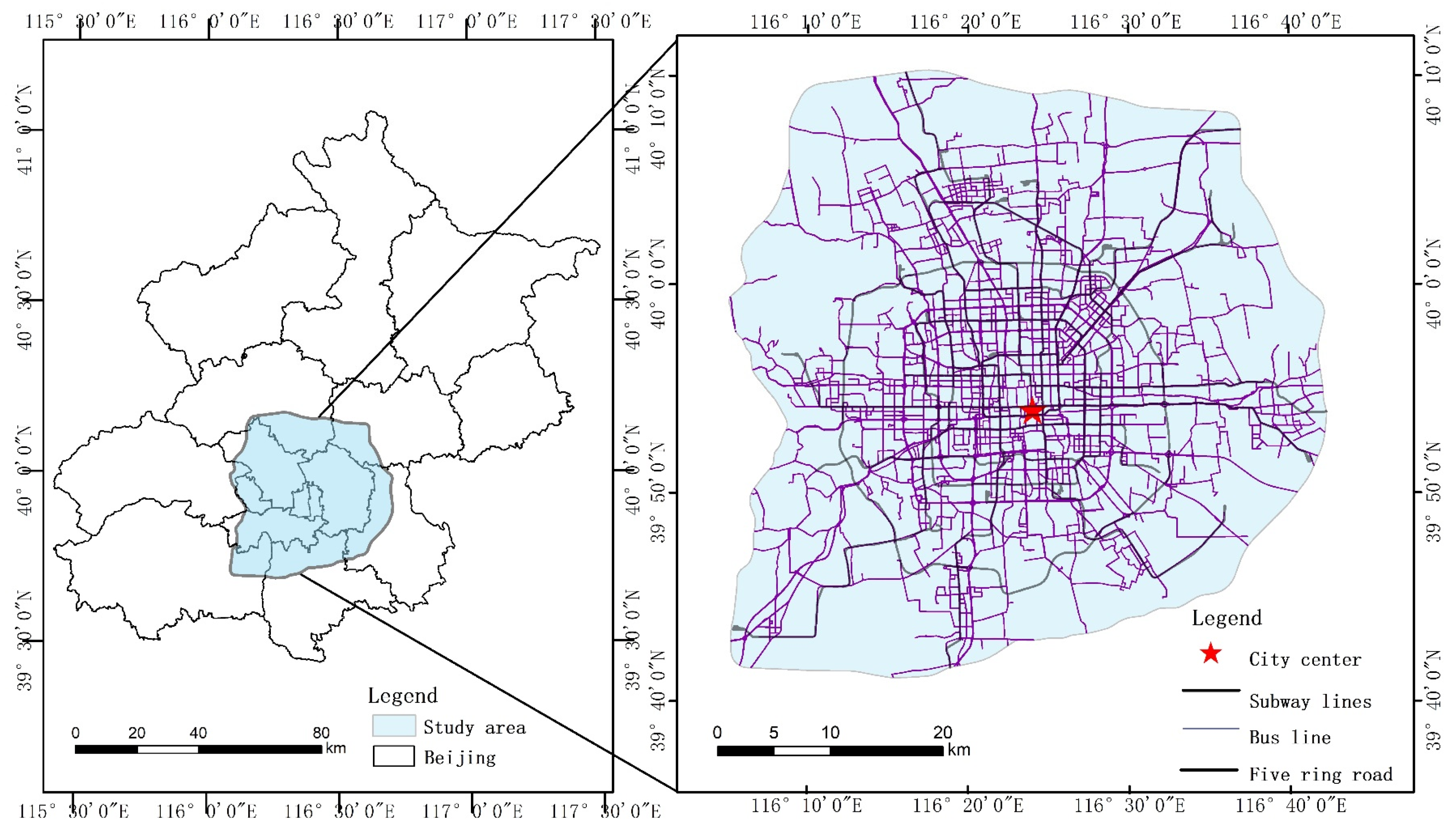
2.1. Study Area

As the capital of China, Beijing City has a huge population, which reached over 21.88 million in 2015. It is one of the main metropolises in China and announced its Public Transit Priority Strategy over 20 years ago. A high level of public transport service has been provided to Beijing residents with dense stations and lines. Over 80% of residents can reach a public transport station within 500 m, and there are over 876 bus lines, 22.69 thousand buses, and 5928 bus stations. Moreover, public transport in Beijing City is dominated by public tram lines and suburban lines, supplemented by rapid bus transit, long-distance lines, customized buses, and tourist lines. There is a large volume of public traffic in Beijing, approximately 20.08 million passengers per day. However, with the rapid population agglomeration, the traffic jams in Beijing have become an issue. Meanwhile, Beijing is decongesting its noncapital functions to promote high quality development. Therefore, it is imperative that the spatial distribution of bus lines should be improved. Urban rail transit in Beijing has been vigorously developed in recent years; however, bus travel is a major mode of public transport in Beijing, accounting for over half of the passenger volume of Beijing’s public transport sector. One possible reason is the different price policies. Since 2007, Beijing has implemented a low-price policy for buses but raised the price of metro travel in 2014.

Considering the line flexibility and the large usage volume, this study will address the bus system in the urban area of Beijing. The Sixth Ring Road of Beijing was selected as the research area, which contains the main urban area of Beijing [27], including 565 bus lines, and 4161 bus stations (Figure 1). To carry out further analysis, the area in the sixth ring will be divided into grid cells. Various cell sizes have been used in previous studies, with the cell size of 1 km × 1 km the most frequent [28]. Thus, a cell size of 1 km × 1 km will be used in this study.

2.2. Data Sources and Processing

The transit flow data, originating from SCD, from April 19 to April 25 in 2015 were obtained from the Beijing Public Transport Group. The SCD contains detailed information on each trip, including the trip id, passenger id, age, boarding and alighting time, and boarding and alighting location. Before dealing with the relevant data, we signed a non-disclosure agreement to protect the personal privacy of the passengers. In addition, any cards which lacked essential information were excluded. The sample records and selected fields of smart card data are shown in

Table 1. Sample records of smart card data.

Time	Card Number	Type	Line Number	Vehicle Number	Boarding Station	Departure Station
75487061	1	622	20150814000000	62026	87501	6
71755266	18	598	20150814000000	331	420099	18

. The SCD were matched to the grid through the bus station location connection. This study processed the data in two steps: First, this study used the data for a week to analyze the temporal changes of flow in a day. The dataset was organized into seven periods from 7:00 to 21:00 every day. Then, the data were separated according to working days and weekends to detect the difference in bus flows between weekdays and weekends.

The first step towards constructing a graph from a bus network is to define what the vertices (nodes) and edges (links) are. For this study, a bus station was not a node if it did not offer a transfer. The adjacent stations were assigned a value of 1, and the others were assigned a value of 0 in the binary symmetric matrix of the bus line networks. The centrality of the line network was calculated based on the MCA model. The line matrix was imported into Pajek software.

The second step is to construct the flow matrix. A bus station needed to match the longitude and latitude coordinates with the grid and link the number of incoming and outgoing passengers. Different from the line matrix, the traffic matrix was a directed network and an asymmetric matrix. In the centrality calculation of the flow network, the traffic volume regarding the number of passengers flowing in and out of the station was put into a 1 km × 1 km grid, and the regional grid within the Sixth Ring Road of Beijing was divided into 2371 grids. A 234 × 2371 weighting matrix was constructed to calculate the weighted centrality of the traffic network. Finally, the correlation between the morphological network and traffic network was analyzed, and this study discussed the coordination between the physical morphological network and the actual traffic flow.

2.3. Methods

Multiple centrality assessment indices have significantly contributed to the understanding of how networks can be classified according to their topological characteristics [29]. Freeman [30] proposed that central nodes were those “in the thick of things” or focal points. He formalized three different measures of node centrality, namely, degree, closeness, and betweenness. In this study, degree centrality, closeness centrality, and betweenness centrality were used to measure the centrality of the bus line network.

The degree centrality (DC) of nodes is the most direct metric for describing node centrality in the network analysis [30,31]. The more degree centrality a node has, the more important it is in the network. Betweenness centrality (BC) refers to the frequency at which a node lies on the shortest path between two other nodes and can funnel the flow in the network [30]. The higher the betweenness centrality, the greater the priority and control of the node. Closeness centrality (CC) measures the distance between a node and all other nodes on the shortest path of a weighted network of public transport flows [32]. The greater the closeness centrality, the more direct the spatial associations are among nodes, and the easier it is for the node to play the role of the center [33,34]. The relevant formulas can be seen in

Table 2. Formulas of indicators regarding the multiple centrality assessment model.

Index	Formula	Number	Explanation
Degree centrality (DC)	$D{C}_i={\displaystyle {\displaystyle \sum }_{j\in v\left(i\right)}}{a}_{ij}$	(1)	where DCi represents the degree centrality of node i, v(i) represents the collection of node numbers, a is a binary value, and a is 1 when node i and node j are connected, otherwise it is 0. Since subway lines are a two-way network, the matrix is a symmetric matrix.
Betweenness centrality (BC)	$B{C}_i=\frac{n-1}{{{\displaystyle \sum }}_{j\in \mathrm{v}\left(i\right)}{d}_{ij}}$	(2)	where $B{C}_i$ is the betweenness centrality of node i, n is the actual number of connections in the network, and dij is the shortest distance between grid i and grid j.
Closeness centrality (CC)	$C{C}_i={{\displaystyle \sum }}_{k\ne i\ne j\in \mathrm{N}}\frac{{\delta }_{kj}\left(i\right)}{{\delta }_{kj}}$	(3)	where $C{C}_i$ is the closeness centrality of node i, ${\delta }_{kj}$ is the number of shortest paths between nodes j and k, and ${\delta }_{kj}\left(i\right)$ is the number of these shortest paths that pass-through node i.

.

The weight of each node is considered in the above three indicators. The weighted degree centrality (WNDC) is defined as the sum of weights and labelled as node strengths [35], which is the passenger flow in and out of the grid in this study. The weighted node betweenness degree (WNBC) is applied to describe the shortest path of a reciprocal weighted graph, reflecting propagation through a chain or showing whether a node is contained in the path with a relatively large stream [29]. In a network weighted by passenger flow, the effective distance metric weights the node closeness centrality (WNCC) [36]. The passenger flow was adopted to weight the bus network in this study.

This study adopted the MCA and weighted MCA model to explore the overall and individual characteristics of bus line networks and bus flow networks, and thus reveal the coordination between them. The relevant formulas can be seen in

Table 3. Formulas of indicators regarding the weighted multiple centrality assessment model.

Index	Formula	Number	Explanation
Weighted node degree centrality (WNDC)	$WND{C}_i^w={\displaystyle {\displaystyle \sum }_{j\in v\left(i\right)}}{a}_{ij}{w}_{ij}$	(4)	where $WND{C}_i^w$ represents the weighted node degree centrality of node i, and $w_{ij}$ represents the weight of traffic flows between grids i and j.
Weighted node betweenness centrality (WNBC)	$WNB{C}_i^w=\min \left(\frac{1}{\left(w_{ih}\right)}+\cdots +\frac{1}{\left(w_{hj}\right)}\right)$	(5)	where $WNB{C}_i^w$ represents the weighted node betweenness centrality of node i, and $w_{ik}$ represents the weight of traffic flows between grids i and k.
Weighted node closeness centrality (WNCC)	$D_{ij}=1-\ln (\raisebox{1ex}{$w_{ij}$}\!\left/ \!\raisebox{-1ex}{${{\displaystyle \sum }}_j{w}_{ij}$}\right.)$ $WNC{C}_i={{\displaystyle \sum }}_{k\ne i\ne j\in \mathrm{N}}\frac{{\gamma }_{kj}\left(i\right)}{{\gamma }_{kj}}$	(6)	where $D_{ij}$ represents the effective distance between node i and j, $w_{ij}$ represents the weight of traffic flows between grids i and j, and Pij is the proportion of information flow from node i to node j. $WNC{C}_i^w$ represents the weighted node closeness centrality of node i, ${\gamma }_{kj}$ is the number of paths with the shortest effective distance between nodes j and k, and ${\gamma }_{kj}\left(i\right)$ is the number of these shortest effective distance paths through node i.

.

Kernel density analysis is used to describe the spatial density characteristics and distribution trend of the research object, which can effectively check the influence degree of the surrounding area. This study used the built-in KDE tool in ArcGIS 10.2, which adopts the popular quartic function [37]. KED was applied to smooth the centrality value of the grid to the surface of the six rings to obtain a continuous spatial distribution map. The KDE equation density distribution is highest at the center of each point and decreases continuously. When the distance from the center reaches a certain threshold range (bandwidth), the density is 0 [38]. KDE should be selected with an appropriate bandwidth; in this study the cell size was set as 100 m × 100 m, and the bandwidth was 3500 m [39]:

$$\widehat{f}\left(x\right)=\frac{1}{nh}{\sum }_{i=1}^{n}K(\frac{x-x_i}{h})$$

(7)

where $\widehat{f}\left(x\right)$ is the kernel density of x point; x_i is the property value; K is the kernel function; h is the bandwidth; and n is the total number of points within the bandwidth.

Spatial autocorrelation is an indicator of the degree of aggregation of the attribute values in a spatial unit, aiming to measure spatially whether a point has an attribute value that is correlated with its neighbor’s. The spatial autocorrelation includes global and local spatial autocorrelation. Anselin [40] proposed that bivariate Moran’s I can effectively reflect the correlation characteristics of the spatial distribution of two types of variables:

$$I=\frac{{\sum }_{i=1}^n{\sum }_j^n{W}_{ij}\left(x_i-\overline{x}\right)\left(y_i-\overline{y}\right)}{S^2{\sum }_{i=1}^n{\sum }_{j=1}^n{W}_{ij}}.$$

(8)

where W_ij is the spatial weight matrix established by the K-adjacency relation method, x_i and y_j are the observed values of independent variables and dependent variables in spatial units i and j, respectively; and S² is the variance of all samples.

The calculation method of bivariate local Moran’s I is as follows:

$$I_i=z_i{\sum }_{j=1}^n{w}_{ij}{z}_j$$

(9)

where Z_i and Z_j are the variance-standardized values of the observed values of space units i and j. I_i contains four clustering patterns, and the resulting LISA (local indications of spatial association) distribution map intuitively shows the agglomeration and differentiation characteristics of independent variables and dependent variables in local areas. The clustering pattern can be divided into four types, namely: H-H (high-high) aggregation, that is, the independent variables of spatial unit i and the dependent variables of adjacent unit j are large; L-L (low-low) aggregation, that is, the independent variable value of spatial unit i and the dependent variable value of adjacent unit j are small; L-H (low-high) aggregation, that is, the independent variable value of spatial unit i is small and the dependent variable value of adjacent unit j is large; and H-L (high-low) aggregation, that is, the independent variable value of spatial unit i is large and the dependent variable value of adjacent unit j is small.

3. Results

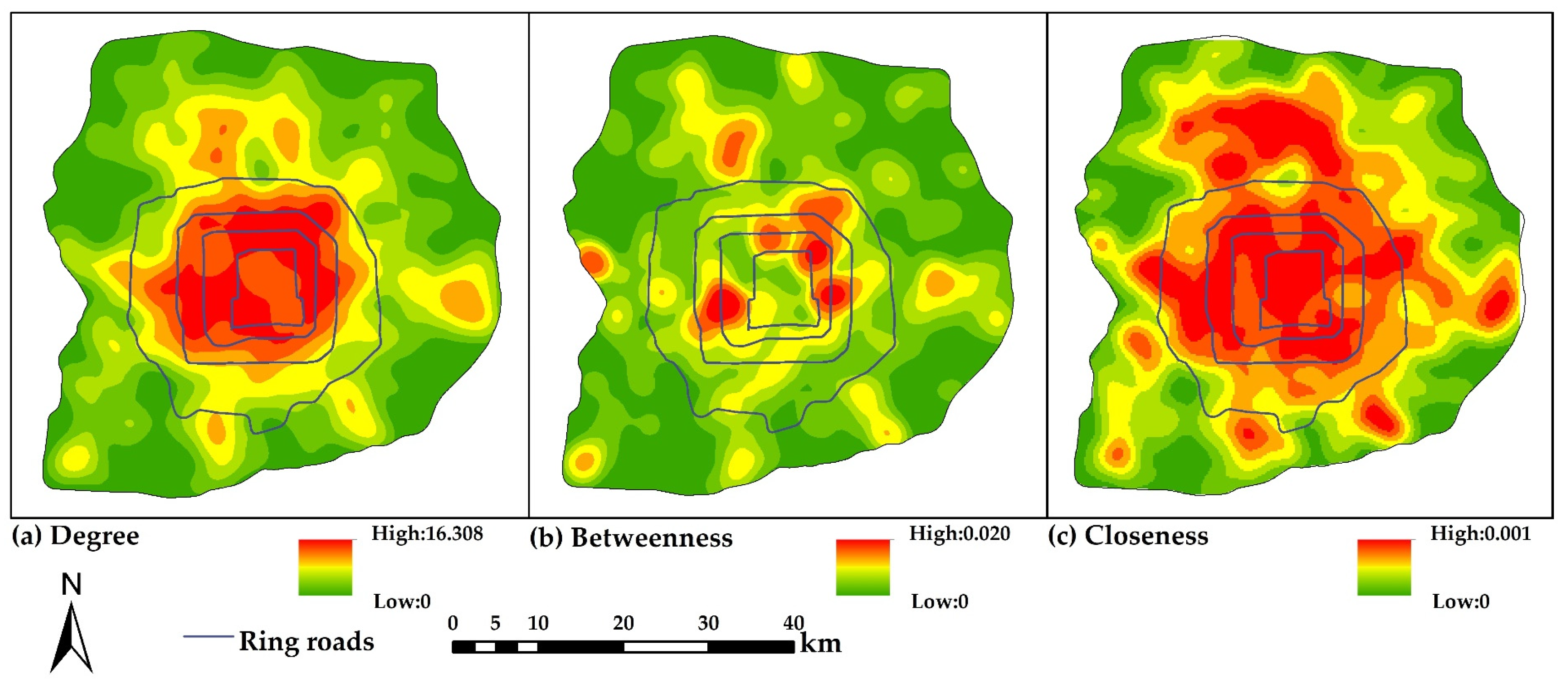
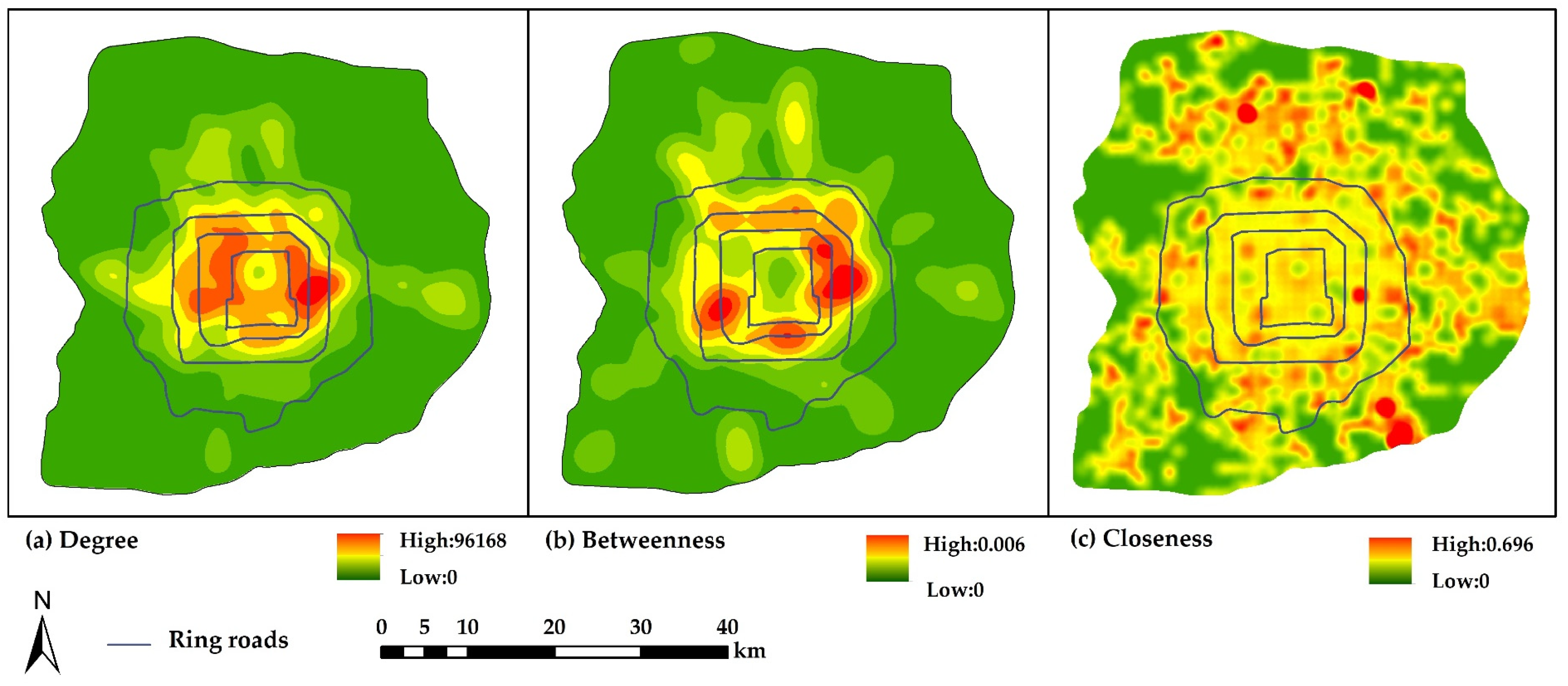
3.1. Centrality of Traffic Line Networks

Figure 2 provides the distribution of the centrality of the bus line networks. The greater the regional interpolation, the warmer the color. Degree centrality and closeness centrality are similar in their spatial distribution characteristics. More specifically, they present high values in the city center and gradually decrease towards the periphery. The high value of degree centrality is distributed within the Fourth Ring Road, indicating that there are more bus stations connected and there are more choices to go to other bus stations. Moreover, the distribution of closeness centrality is wider than that of degree centrality.

In contrast with degree centrality and closeness centrality, betweenness centrality presents a lower value in the second ring. There is a high betweenness centrality value in Beijing West Railway Station, Beijing Railway Station, Sanlitun, and Zhongguancun, which shows that these places have a strong ability to control the city’s public transportation network, and there are more transit stations.

Figure 3 presents the centrality distribution in the bus network weighted by passenger flow, that is, weighted degree centrality, weighted betweenness centrality and weighted closeness centrality. The centrality of the weighted degree is low in Beihai Park within the Second Ring Road, and the highest value appears near Beijing CBD in Chaoyang District. The weighted betweenness centrality is high in the Beijing CBD, Beijing West Railway Station and Beijing South Railway Station, indicating that these places have stronger links and easier access. The weighted closeness centrality measured by effective distance presents a decentralized cluster distribution in spatial distribution. The lower the proportion of node outflow in the total flow, the farther the distance. The smaller the total distance between the node and other nodes, the more concentrated the outflow from the node.

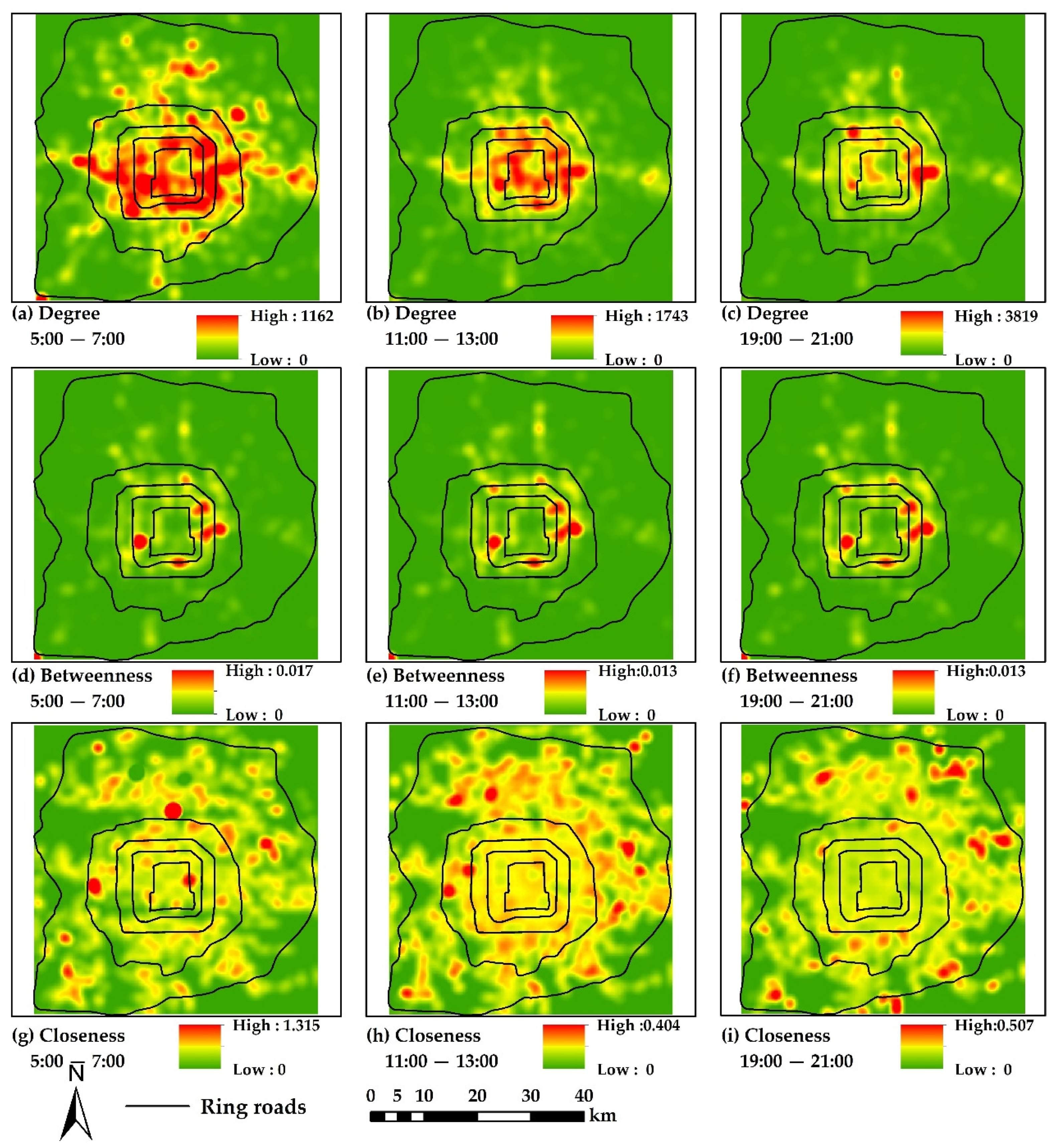
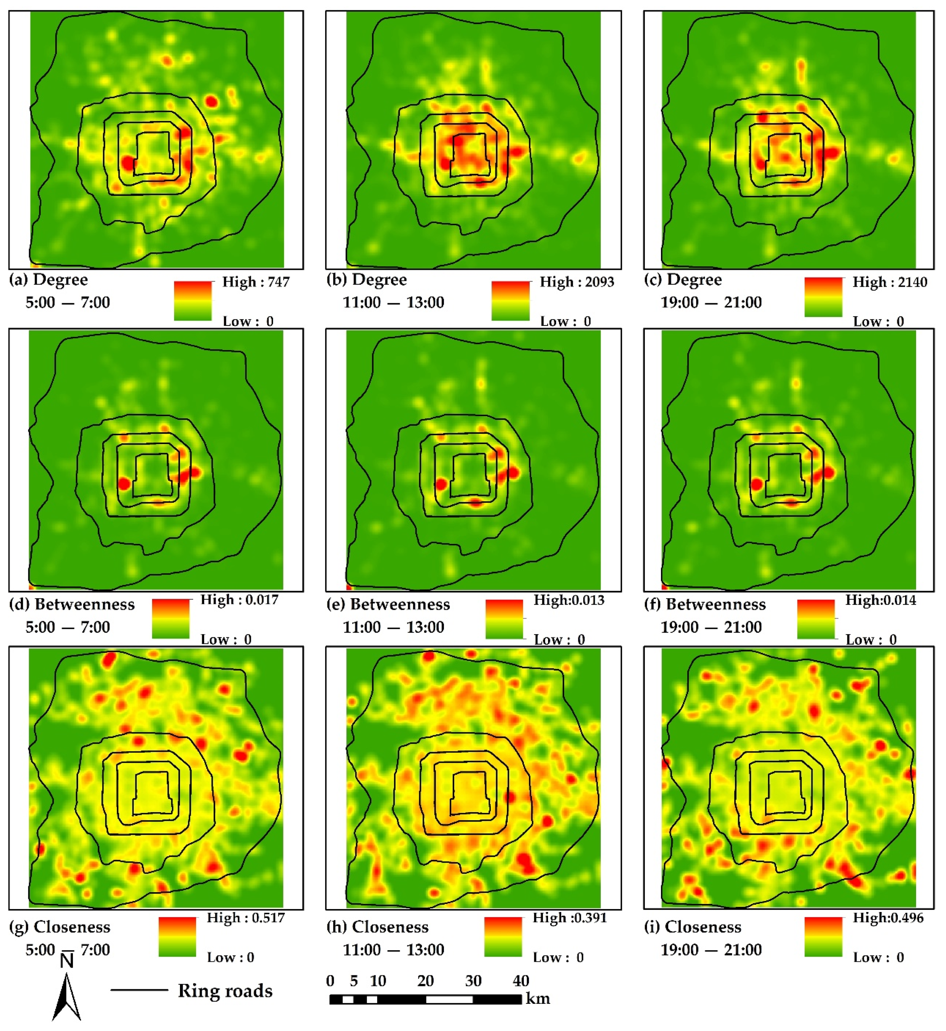
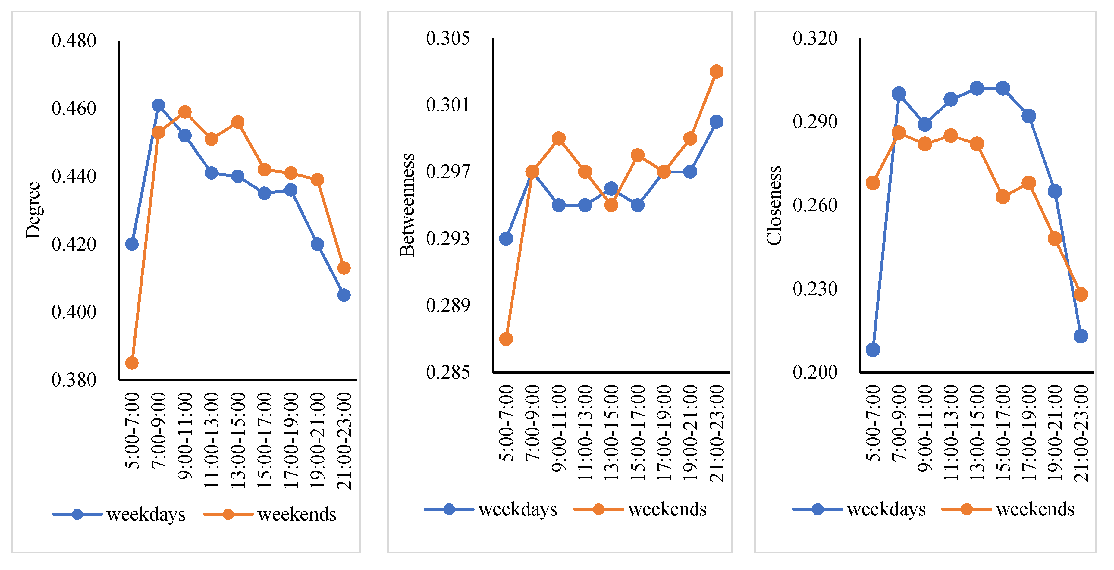
3.2. Temporal Variations in the Centrality of Flow Networks

The weighted centrality from 5:00 a.m. to 23:00 p.m. in a day, divided by two hour-periods, on weekdays and the weekend, was calculated. This study divided into three of these periods, including 7:00 a.m. to 9:00 a.m., 11:00 p.m. to 13:00 p.m., and 19:00 p.m. to 21:00 p.m. Figure 4 shows the distribution of three types of centralities in three periods of weekdays.

The centrality of the weighted degree is calculated based on the number of outgoing passengers in the grid. The range of distribution in the three periods gradually decreases. This reflects the difference between the place of residence and the workplace. The flow from 5:00 a.m. to 7:00 a.m. is mainly from the place of residence, and that from 19:00 p.m. to 21:00 p.m. is mainly from the place of work.

The change in weighted betweenness centrality is small. The stable multicore-high distribution includes the Beijing West Railway Station, CBD, among others. The weighted betweenness centrality of Zhongguancun increases significantly in the latter two periods, revealing that these places have strong links and are more accessible.

The more dispersed the passenger flow is from the grid, the longer the effective distance. Therefore, the higher the compactness centrality is when measured by effective distance, the more concentrated the inflow of passenger flow in the grid.

Figure 5 shows the distribution of three types of centralities in three periods of weekends. In contrast with the weighted degree centrality on weekdays, the weighted degree centrality reveals the characteristics of a high value range from 7:00 AM to 17:00 PM on weekends. Compared with weekdays, there are more stable passenger flows. Weighted betweenness centrality changes little on weekdays and weekends. In Zhongguancun, the weighted betweenness centrality shows a stable, high value on the weekends.

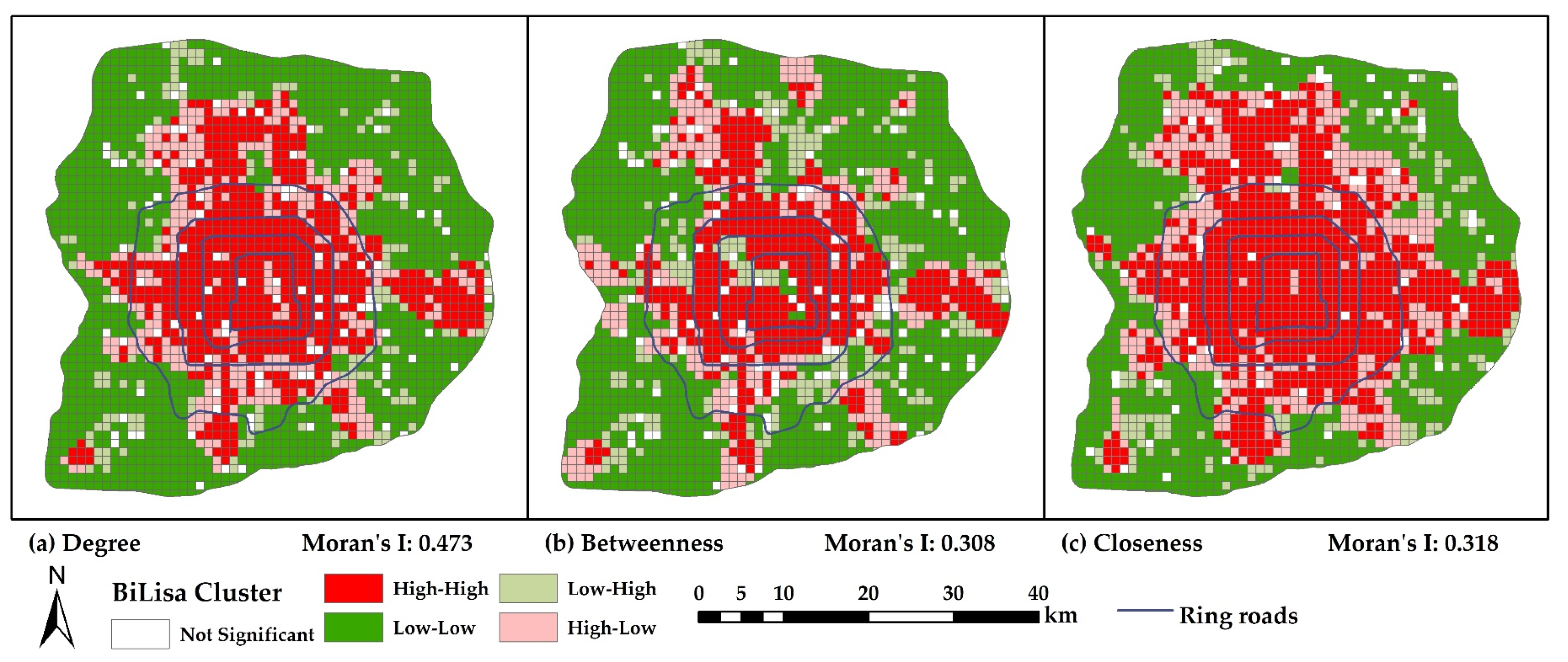
3.3. The Relationship between Line Network Centrality and Flow Networks

To explore the relationship between the centrality of the bus lines network and the centrality of the bus flow network, the bivariate Moran’s I was used in this study (Figure 6). Considering the distance between grids or the resident population in the grid as the spatial weight matrix, both passed the significance test. The insignificant grid proportion with population as the spatial weight matrix is less than with the spatial weight matrix measured by distance. Therefore, the population in the grid was selected as the spatial weight matrix.

On weekdays, the degree centrality and closeness centrality of the bivariate Moran’s I are small from 5:00 AM to 7:00 AM and reach a small peak from 7:00 AM to 9:00 AM. Then, both the bivariate Moran’s I of degree centrality and closeness centrality show a downwards trend. The bivariate Moran’s I of betweenness centrality shows an upwards trend throughout the day. For the bivariate Moran’s I of degree centrality, the value is small from 5:00 AM to 7:00 AM. During the morning peak from 7:00 AM to 9:00 AM, the bivariate Moran’s I of degree centrality reaches the peak (0.461). Then, it gradually shows a downwards trend until the evening peak from 17:00 PM to 19:00 PM, with a small increase to 0.436 and then continues to decline. The bivariate Moran’s I of betweenness centrality shows an upwards overall trend, in which 5:00 AM to 7:00 AM is the lowest value (0.293), reaches a small peak (0.297) from 7:00 AM to 9:00 AM, decreases slightly from 9:00 to 11:00, and then shows an upwards trend. Ultimately, the bivariate Moran’s I of betweenness centrality reaches the highest value (0.300) from 21:00 PM to 23:00 PM at night. The value of the bivariate Moran’s I of closeness centrality is 0.208 from 5:00 to 7:00 and presents a sharp increase (0.300) from 7:00 AM to 9:00 AM. There is a small decrease from 9:00 AM to 11:00 AM, down to 0.289. Then, it presents an upwards trend, reaching a peak of 0.302 at 15:00 PM–17:00 PM.

On the weekend, the bivariate Moran’s I shows a relatively low value in degree centrality and closeness centrality from 5:00 AM to 7:00 AM and then begins to rise, showing a fluctuating downwards trend. The bivariate Moran’s I of betweenness centrality presents the lowest value from 5:00 AM to 7:00 AM and then shows a fluctuating upwards trend. The minimum value of the bivariate Moran’s I of degree centrality is 0.385 from 5:00 AM to 7:00 AM. It rises rapidly from 7:00 AM to 9:00 AM and reaches 0.453. The peak value is 0.459 from 9:00 AM to 11:00 AM. The bivariate Moran’s I of degree centrality decreases slightly from 11:00 AM to 13:00 PM (0.451), reaches a small peak from 13:00 PM to 15:00 PM (0.456), and then gradually decreases. The bivariate Moran’s I of betweenness centrality presents two peaks at 9:00 AM–11:00 AM and 17:00 PM–19:00 PM and reaches the maximum value of 0.303 at 21:00 PM-23:00 PM. The value of closeness centrality is 0.268 at 5:00 AM–7:00 AM, reaches the peak value of 0.286, and then declines with some fluctuation.

Generally, the changing trend of the bivariate Moran’s I of the three central indices is the same on weekdays and weekends. The difference is that the bivariate Moran’s I of degree centrality and betweenness centrality on weekdays are lower than those on weekends. The bivariate Moran’s I of closeness centrality on weekends is lower than that on weekdays.

Table 4. Comparison of bivariate spatial autocorrelation peaks of line networks and traffic networks.

Type	Weekdays	Weekends
Degree	0.461 (7:00–9:00)	0.459 (9:00–11:00)
Betweenness	0.302 (15:00–17:00)	0.286 (7:00–9:00)
Closeness	0.302 (15:00–17:00)	0.286 (7:00–9:00)

shows the highest values of the bivariate Moran’s I of the three types of centralities. The highest value of degree centrality on weekdays occurs from 7:00 AM to 9:00 AM, and the highest value on weekends is delayed (9:00 AM–11:00 AM). The highest values of betweenness centrality and closeness centrality appear from 15:00 PM–17:00 PM on weekdays and from 7:00 AM–9:00 AM on weekends.

Figure 7 shows the spatial difference and correlation of the bus line network and bus flow network measured by bivariate Moran’s I. The spatial distribution of bivariate Moran’s I by the three types of centralities of distance is similar. High-High grids are mainly distributed within the Fifth Ring Road and residential areas such as Fangshan District and Tongzhou District. LH outliers are mainly distributed in residential areas such as Changyang town, Fangshan District, Shahe station and Shahe town, and Changping District. The regional distribution of HL outliers is mainly along the Fifth Ring Road, northwest Wangzhen, Zhongguancun Park, Yongfeng Township, and other places in the northwest, which is characterized by its distribution around the HH area.

4. Discussion and Conclusions

4.1. General Discussion

The objective in this study is to explore the correlation between the network of urban bus lines and the flow network on it. Based on SCD data, a network of bus lines and bus flows was constructed, and the complex network analysis approach was employed to examine the spatial patterns of the networks. Three kinds of node centrality indices were calculated and compared. The results are as follows:

First, the overall spatial patterns of node centralities between the bus line network and the bus flow network were similar, while there were also some differences to a certain degree. This further reveals that the flow of passengers in Beijing City has been taken into account in the construction of public bus lines. In other words, the design of public bus lines in Beijing is relatively favorable;

Secondly, when comparing the static structure of the bus line network with the dynamic structure of the bus flow network, the differences varied with time, such as between weekends and weekdays, or at different hours of the day. The spatial centrality pattern of the bus line network has a higher correlation with the flow network at the morning peak hours of 7:00 AM to 9:00 AM on weekdays and at 9:00 AM to 11:00 AM on weekends. This can be explained by the fact that, given the traffic jams, passengers may mainly choose public transportation to arrive at their workplaces in time in metropolitan areas; Thirdly, the areas of the type high-low or type low-high are mainly distributed at the edge of type high-high areas, which are mostly also at the edge of the main built-up areas of Beijing. This implies that the match of the two networks is relatively good in urban areas and rural areas but relatively poor in the transition zones between them. In other words, the relationship between the bus line organization and the passenger flow network is not coordinated in metropolitan suburban areas. Either there is a lack of bus lines, or the scale of passenger flow is relatively smaller.

4.2. Theoretical Contributions

Our study makes the following contribution: First, this study further enriches the content on the change in network characteristics with time. Secondly, the application of bus-card swiping data with a large sample size and high precision provides an objective basis for interpreting the dynamic characteristics of bus passenger flow networks. Thirdly, this research is of great significance for enhancing the capability of urban management, and further promoting the science of urban traffic planning. More importantly, a research framework that integrates complex network analysis and GIS spatial analysis is universal and can be applied to the investigation of bus lines and flows across other urban metropolitan areas in the world.

4.3. Practical Implications

According to the main conclusions, this study provides the following recommendations. First, against the background regarding deconstruction of noncapital functions, the bus lines need to be enhanced in an orderly fashion based on the flows, especially in regions with high volumes of passenger traffic. If possible, dynamic changes between holidays or within a day should be noticed by transport planning authorities. Secondly, the running time of buses on holidays should be enhanced in the areas around train stations and airports to promote the supply capacities of bus systems for passenger flows. Thirdly, the mismatch situation mostly occurs at the transition zones at the city edge, which should be given more attention by bus service planning authorities.

References

1. Macioszek, E.; Kurek, A. P&R parking and bike-sharing system as solutions supporting transport accessibility of the city. Transp. Probl. 2020, 15, 275–286. [Google Scholar] [CrossRef]
2. Soomro, R.; Memon, I.A.; Pathan, A.F.H.; Mahar, W.A.; Sahito, N.; Lashari, Z.A. Factors That Influence Travelers’ Willingness to Adopt Bus Rapid Transit (Green Line) Service in Karachi. Sustainability 2022, 14, 10184. [Google Scholar] [CrossRef]
3. Macioszek, E.; Cieśla, M. External Environmental Analysis for Sustainable Bike-Sharing System Development. Energies 2022, 15, 791. [Google Scholar] [CrossRef]
4. Wang, L.-N.; Wang, K.; Shen, J.-L. Weighted complex networks in urban public transportation: Modeling and testing. Phys. A Stat. Mech. Appl. 2019, 545, 123498. [Google Scholar] [CrossRef]
5. Porta, S.; Crucitti, P.; Latora, V. The Network Analysis of Urban Streets: A Primal Approach. Environ. Plan. B Plan. Des. 2006, 33, 705–725. [Google Scholar] [CrossRef] [Green Version]
6. Du, Z.; Tang, J.; Qi, Y.; Wang, Y.; Han, C.; Chunyang, H. Identifying critical nodes in metro network considering topological potential: A case study in Shenzhen city—China. Phys. A Stat. Mech. Appl. 2019, 539, 122926. [Google Scholar] [CrossRef]
7. Chen, Y.-Z.; Li, N.; He, D.-R. A study on some urban bus transport networks. Phys. A Stat. Mech. Appl. 2007, 376, 747–754. [Google Scholar] [CrossRef]
8. Soh, H.; Lim, S.; Zhang, T.; Fu, X.; Lee, G.K.K.; Hung, T.G.G.; Di, P.; Prakasam, S.; Wong, L. Weighted complex network analysis of travel routes on the Singapore public transportation system. Phys. A Stat. Mech. Appl. 2010, 389, 5852–5863. [Google Scholar] [CrossRef]
9. Yang, X.-H.; Chen, G.; Chen, S.-Y.; Wang, W.-L.; Wang, L. Study on some bus transport networks in China with considering spatial characteristics. Transp. Res. Part A Policy Pr. 2014, 69, 1–10. [Google Scholar] [CrossRef]
10. Zhong, C.; Arisona, S.M.; Huang, X.; Batty, M.; Schmitt, G. Detecting the dynamics of urban structure through spatial network analysis. Int. J. Geogr. Inf. Sci. 2014, 28, 2178–2199. [Google Scholar] [CrossRef]
11. Liu, C.; Duan, D. Spatial inequality of bus transit dependence on urban streets and its relationships with socioeconomic intensities: A tale of two megacities in China. J. Transp. Geogr. 2020, 86, 102768. [Google Scholar] [CrossRef]
12. Cardillo, A.; Scellato, S.; Latora, V.; Porta, S. Structural properties of planar graphs of urban street patterns. Phys. Rev. E 2006, 73, 066107. [Google Scholar] [CrossRef] [PubMed] [Green Version]
13. Lin, J.; Ban, Y. Complex Network Topology of Transportation Systems. Transp. Rev. 2013, 33, 658–685. [Google Scholar] [CrossRef]
14. Zhang, M.; Huang, T.; Guo, Z.; He, Z. Complex-network-based traffic network analysis and dynamics: A comprehensive review. Phys. A Stat. Mech. Appl. 2022, 2022, 128063. [Google Scholar] [CrossRef]
15. Luo, D.; Cats, O.; van Lint, H.; Currie, G. Integrating network science and public transport accessibility analysis for comparative assessment. J. Transp. Geogr. 2019, 80, 102505. [Google Scholar] [CrossRef] [Green Version]
16. Xu, Q.; ZU, Z.; Xu, Z.; Zhang, W.; Zheng, T. Space P-Based Empirical Research on Public Transport Complex Networks in 330 Cities of China. J. Transp. Syst. Eng. Inf. Technol. 2013, 13, 193–198. [Google Scholar] [CrossRef]
17. Wan, D.; Huang, Y.; Feng, J.; Shi, Y.; Guo, K.; Zhang, R. Understanding Topological and Spatial Attributes of Bus Transportation Networks in Cities of Chongqing and Chengdu. Math. Probl. Eng. 2018, 2018, 4137806. [Google Scholar] [CrossRef] [Green Version]
18. Zhu, L.; Luo, J. The Evolution Analysis of Guangzhou Subway Network by Complex Network Theory. Procedia Eng. 2016, 137, 186–195. [Google Scholar] [CrossRef] [Green Version]
19. Zhang, L.; Lu, J.; Fu, B.-B.; Li, S.-B. Dynamics analysis for the hour-scale based time-varying characteristic of topology complexity in a weighted urban rail transit network. Phys. A Stat. Mech. Appl. 2019, 527, 121280. [Google Scholar] [CrossRef]
20. Gao, S.; Wang, Y.; Gao, Y.; Liu, Y. Understanding Urban Traffic-Flow Characteristics: A Rethinking of Betweenness Centrality. Environ. Plan. B Plan. Des. 2013, 40, 135–153. [Google Scholar] [CrossRef]
21. Wu, Y.; Wang, L.; Fan, L.; Yang, M.; Zhang, Y.; Feng, Y. Comparison of the spatiotemporal mobility patterns among typical subgroups of the actual population with mobile phone data: A case study of Beijing. Cities 2020, 100, 102670. [Google Scholar] [CrossRef]
22. Ding, R.; Ujang, N.; Bin Hamid, H.; Manan, M.S.A.; Li, R.; Albadareen, S.S.M.; Nochian, A.; Wu, J. Application of Complex Networks Theory in Urban Traffic Network Researches. Netw. Spat. Econ. 2019, 19, 1281–1317. [Google Scholar] [CrossRef]
23. Xu, Q.; Mao, B.; Bai, Y. Network structure of subway passenger flows. J. Stat. Mech. Theory Exp. 2016, 2016, 033404. [Google Scholar] [CrossRef] [Green Version]
24. Meng, Y.; Tian, X.; Li, Z.; Zhou, W.; Zhou, Z.; Zhong, M. Exploring node importance evolution of weighted complex networks in urban rail transit. Phys. A Stat. Mech. Appl. 2020, 558, 124925. [Google Scholar] [CrossRef]
25. Feng, J.; Li, X.; Mao, B.; Xu, Q.; Bai, Y. Weighted complex network analysis of the Beijing subway system: Train and passenger flows. Phys. A Stat. Mech. Appl. 2017, 474, 213–223. [Google Scholar] [CrossRef]
26. Wang, Y.; Deng, Y.; Ren, F.; Zhu, R.; Wang, P.; Du, T.; Du, Q. Analysing the spatial configuration of urban bus networks based on the geospatial network analysis method. Cities 2020, 96, 102406. [Google Scholar] [CrossRef]
27. Liao, C.; Dai, T.; Zhao, P.; Ding, T. Weighted Centrality and Retail Store Locations in Beijing, China: A Temporal Perspective from Dynamic Public Transport Flow Networks. Appl. Sci. 2021, 11, 9069. [Google Scholar] [CrossRef]
28. Li, Q.; Zhou, S.; Wen, P. The relationship between centrality and land use patterns: Empirical evidence from five Chinese metropolises. Comput. Environ. Urban Syst. 2019, 78, 101356. [Google Scholar] [CrossRef]
29. Opsahl, T.; Agneessens, F.; Skvoretz, J. Node centrality in weighted networks: Generalizing degree and shortest paths. Soc. Netw. 2010, 32, 245–251. [Google Scholar] [CrossRef]
30. Freeman, L.C. Centrality in social networks conceptual clarification. Soc. Netw. 1978, 1, 215–239. [Google Scholar] [CrossRef]
31. Wang, J.; Li, C.; Xia, C. Improved centrality indicators to characterize the nodal spreading capability in complex networks. Appl. Math. Comput. 2018, 334, 388–400. [Google Scholar] [CrossRef]
32. Sabidussi, G. The centrality index of a graph. Psychometrika 1966, 31, 581–603. [Google Scholar] [CrossRef] [PubMed]
33. Liu, Q.; Song, J.; Dai, T.; Xu, J.; Li, J.; Wang, E. Spatial Network Structure of China’s Provincial-Scale Tourism Eco-Efficiency: A Social Network Analysis. Energies 2022, 15, 1324. [Google Scholar] [CrossRef]
34. Lü, L.; Zhang, Y.-C.; Yeung, C.H.; Zhou, T. Leaders in Social Networks, the Delicious Case. PLoS ONE 2011, 6, e21202. [Google Scholar] [CrossRef] [Green Version]
35. Barrat, A.; Barthelemy, M.; Pastor-Satorras, R.; Vespignani, A. The architecture of complex weighted networks. Proc. Natl. Acad. Sci. USA 2004, 101, 3747–3752. [Google Scholar] [CrossRef] [Green Version]
36. Brockmann, D.; Helbing, D. The hidden geometry of complex, network-driven contagion phenomena. Science 2013, 342, 1337–1342. [Google Scholar] [CrossRef] [Green Version]
37. Silverman, B.W. Density Estimation for Statistics and Data Analysis; Routledge: New York, NY, USA, 2018. [Google Scholar]
38. Wang, F.; Antipova, A.; Porta, S. Street centrality and land use intensity in Baton Rouge, Louisiana. J. Transp. Geogr. 2011, 19, 285–293. [Google Scholar] [CrossRef] [Green Version]
39. Lin, G.; Chen, X.; Liang, Y. The location of retail stores and street centrality in Guangzhou, China. Appl. Geogr. 2018, 100, 12–20. [Google Scholar] [CrossRef]
40. Anselin, L. The Local Indicators of Spatial Association—LISA. Geogr. Anal. 1995, 27, 93–115. [Google Scholar] [CrossRef]
Figure 1. Case study area.
Sustainability 14 15454 g001
Figure 2. The spatial distribution of the centrality of the bus line network.
Sustainability 14 15454 g002
Figure 3. The spatial distribution of the weighted centrality of the bus flow network.
Sustainability 14 15454 g003
Figure 4. The spatial distribution of the weighted degree centrality of bus flow networks on weekdays.
Sustainability 14 15454 g004
Figure 5. The spatial distribution of the weighted degree centrality of bus flow networks on weekends.
Sustainability 14 15454 g005
Figure 6. Temporal variations of the bivariate Moran’s I between the centrality indices and weighted centrality indices on weekdays and weekends. (Left: degree; Middle: betweenness; and Right: closeness).
Sustainability 14 15454 g006
Figure 7. Bivariate Moran’s I of centrality in the bus line network and flow network.
Sustainability 14 15454 g007