A Study on Optimal Location Selection and Semi-Finished Product Inventory Allocation in the Steel Industry

Abstract

With the development of industrial production technologies and market economy, Postponement is increasingly being adopted by continuous production enterprise as a method that enables multi-product, mass customization production. In order to make use of the Postponement in manufacturing production enterprises need to achieve customized production and reduce enterprise costs. A modeling is conducted in the production process of Postponement in iron and steel enterprises in this paper. With the goal of minimizing total costs on a specific customer service level, mixed integer nonlinear programming and particle swarm algorithms are adopted for modeling and solving, to determine the optimal location and optimal semi-finished product inventory of PDP and CODP. Finally, taking an iron and steel enterprise as an example, the feasibility and effectiveness of the model and algorithm are verified. The study shows that the change of the optimal locations of PDP and CODP is affected by the change of customer service level and delay penalty coefficient, but the speed of change of the optimal location of PDP shows longer delays. In addition, the size of the capacity of semi-finished product inventory corresponding to CODP has a direct influence on whether the semi-finished product inventory corresponding to PDP participates in production, which in turn affects the optimal semi-finished product inventory on all levels. Through the analysis, it is found that the model constructed in this paper can better describe the overall situation and the influence relationship of the Postponement, and the study supplements the deficiency of the research on Postponement in the continuous manufacturing enterprises and enriches the content of the quantitative research on the Postponement.

1. Introduction

Iron and steel enterprises are typical continuous manufacturing enterprises, with high continuity in production, various process routes, and high product diversification. Besides, the industry is one of the main players regarding carbon emission production [1,2]. Therefore, responsible production planning is a key issue also from sustainability aspect. In the past, iron and steel enterprises mainly adopted the make-to-stock mode (MTS) and the make-to-order mode (MTO) for production [3,4]. MTS has the advantages of high production efficiency, low production cost and fast delivery, but it cannot meet the needs of product diversification and customization. MTO has the advantages of adapting to product diversification and customization, although with low production efficiency and slow delivery. Generally, MTO brings higher production cost. Neither of the two production modes can effectively meet the current production requirements of iron and steel enterprises. Postponement has been widely applied in enterprises as an effective way to realize mass product customization, and the optimization of Postponement has also received more attention from business and academic circles [5,6].

Production mode refers to the form and operation mode of enterprise system, operation, management, etc. In this article, it mainly refers to the inventory management rules and production scheduling sequence [7]. An effective production mode can promote enterprises to improve efficiency and reduce costs. At present, for various manufacturing enterprises, it is an important development trend to use Industry 4.0 to optimize production plans and processes to achieve mass customization and diversified production [8,9]. For iron and steel enterprises, the main way of this optimization is Postponement, which is also the optimization of production control process [10].

Postponement is a production strategy that appropriately delays production links such as production, assembly, distribution, and transportation. The subsequent production strategy will not be completed until the customer order arrives. Postponement originates from supply chain management and was mainly used to realize customized production and balance production cost and production time. Later, with the improvement of marketization, the development of information technology, and the progress of production technology, the Postponement is widely used in enterprise production [11]. At present, with the promotion of Industry 4.0, more enterprises use the Postponement to achieve large-scale customization [12,13]. This production mode can be seen as an integration of MTO and MTS. In contrast with MTO, the Postponement has higher production efficiency and lower production cost. Compared with MTS, it can better meet the needs of product diversification and customization [13]. In enterprises that engage in continuous manufacturing of iron and steel, the Postponement is mainly applied in cases of production delay, where the goal is to achieve continuous, multi-product, customized production. For a production process there are often multiple points at which unique property changes can be determined, called points of decoupling (DP). Different types of decoupling points are used to divide control modes, production modes, production continuity, etc. [14]. Among them, the customer order decoupling point (CODP) is the basis for differentiating different production modes (ETO, MTO, ATO, MTS), and it is also the focus of the research and control of Postponement [15,16].

The Postponement in iron and steel enterprises mainly includes two steps. The first step can be called “production preparation stage”; that is, the initial production capacity is converted into a different semi-finished products inventory, including general semi-finished product inventory corresponding to PDP and dedicated semi-finished product inventory corresponding to CODP. The second step can be called the “order fulfillment phase”, which is to use the general semi-finished product inventory and the dedicated semi-finished product inventory to complete the production of the product according to the customer’s order requirements. Among them, the location of the dedicated semi-finished product inventory is related to the location of CODP, while the location of the general semi-finished product inventory is related to the location of PDP. PDP as a product differentiation point refers to the starting point for product differentiation in a certain product category. The location of PDP can affect the unit cost of production and production time of all products in this product category. The semi-finished product inventory corresponding to PDP can affect production costs and customer order fulfillment cycle times for all products in the product category under specific customer needs. CODP as the customer order decoupling point stands for the starting point for enterprises to start production according to customer orders. The location of CODP can affect the unit cost of production and production time of this kind of product. The semi-finished product inventory corresponding to CODP can affect the production costs and customer order fulfillment cycle times for such products under specific customer needs. Therefore, for the use of Postponement in continuous manufacturing enterprises, the locations of PDP and CODP and their corresponding semi-finished product inventory are important means to adjust the production time and costs.

Previous optimization studies on Postponement mostly aimed at continuous manufacturing enterprises, focusing on the positioning of PDP and CODP, and often without considering anything about the influence of semi-finished product inventory. Daaboul et al. [17] studied the influence of the optimal locations of CODP and PDP on Postponements in continuous manufacturing enterprises. Immawan and Arkeman [18] studied the optimal location of CODP for Postponement in continuous manufacturing enterprises in different scenarios but did not consider the influence of the location of PDP and semi-finished product inventory. Ji, Qi, and Gu [19] and Zandieh and Motallebi [20] studied the Postponement of process manufacturing enterprises, and only analyzed the optimal position of CODP without considering the influence of CODP on semi-finished product inventory. Referring to previous research methods and cases, this paper studies the Postponement in continuous manufacturing enterprises, comprehensively considers the influence of PDP and CODP locations and their semi-finished product inventory on the Postponement, and also determines the optimal location and inventory by establishing a quantitative model to balance the production time and total costs.

The model built in this paper is large-scale mixed integer programming. The decision variables include discrete variables and continuous variables solved by an exact algorithm that is slow in operation and complicated in programming. Kitayama and Yasuda [21] show that PSO is a method for holistic or quasi-minimum for nonlinear, non-convex optimization problems, which is high in accuracy and fast in solving mixed integer programming problems. Şahin and Kellegoz [22] used particle swarm algorithm, tabu and cuckoo search to solve the mixed integer programming problem. The study shows that particle swarm algorithm is more advantageous in solving speed and accuracy, thereby used in this paper to solve the model.

The main contributions of this paper are as follows: First, combining the problems in the production of iron and steel enterprises, it complements the lack of research on Postponement in continuous manufacturing enterprises. The second is to conduct quantitative research on the optimization of Postponement. Thirdly, it considers a variety of control contents, and effectively describes the overall situation of Postponement and the impact of various factors on the control contents. Its research results can be better applied to other continuous manufacturing enterprises such as glass manufacturing, chemical manufacturing, food processing, etc.

The innovations of this study lie in three aspects: first, it considers, in a continuous manufacturing enterprise, the influence of the locations of PDP and CODP as well as semi-finished product inventory on Postponement; second, it is found that the change of the optimal locations of PDP and CODP is affected by the change of customer service level and delay penalty coefficient, but the speed of change of the optimal location of PDP shows longer delays; third, it is further found that the size of the capacity of semi-finished product inventory corresponding to CODP has a direct influence on whether the semi-finished product inventory corresponding to PDP participates in production, which in turn affects the optimal semi-finished product inventory at all levels.

The rest of this paper is as follows: Section 2 introduces the research status and insufficiency of the literature related to the content of this paper; Section 3 introduces the production process and features of Postponement in iron and steel enterprises, outlines the research questions of this paper, designs various parameters and variables, and builds a mixed integer nonlinear programming model according to the needs of modeling; Section 4 introduces the heuristic algorithm used for model solution, compares the heuristic algorithm with the exact algorithm, and solves large-scale cases based on the actual data of an iron and steel enterprise; Section 5 discusses and analyzes the relevant influencing factors; Section 6 presents the conclusions.

2. Literature Review

Currently, numerous studies have been conducted on continuous manufacturing enterprises and supply chains related to Postponement than on continuous manufacturing enterprises. The reason behind that is that in actual production, Postponement is widely applied in continuous manufacturing enterprises and supply chains. However, with the development of market economy and the intensification of competition among enterprises, Postponement has been more often introduced to continuous manufacturing enterprises, and the study of such production mode in continuous manufacturing enterprises has also received more and more attention in the academia.

2.1. Studies on Postponement

After reading a large volume of literature on Postponement, we made statistics and analysis of 50 related sources (as shown in

Table 1. Statistics of key research points of papers on Postponement.

	CODP	PDP	Inventory Management	CODP and Inventory Management	CODP and PDP	Others
Supply Chain Management	11	1	1	4	0	4
Discrete Manufacturing Enterprises	11	3	0	3	1	5
Continuous Manufacturing Enterprises	3	0	0	1	0	2
Total	25	4	1	8	1	11

) and found that the research on the Postponement mainly includes three aspects: supply chain management, discrete manufacturing enterprises, and continuous manufacturing enterprises. Most of the publications studied the CODP location, and a small number of texts studied the PDP location and inventory management. There are few sources considering CODP and inventory management at the same time, and even less considering CODP and PDP at the same time. According to the characteristics of Postponement in manufacturing production enterprises, this paper also considers PDP, CODP and semi-finished product inventory management and divides the studies of Postponement into two categories: studies of Postponement in continuous manufacturing enterprises or supply chains, and those of Postponement in continuous manufacturing enterprises.

(1)

Most of the existing literature on Postponement aimed at continuous manufacturing enterprises or supply chains, focusing on the positioning of CODP and PDP and semi-finished product inventory on all levels.

Part of the literature focused on the positioning of the customer order decoupling point (CODP). Ramón-Lumbierres et al. [23], Immawan and Arkeman [18], Wang and Chen [24], Qian [25], and Man [26] combined the characteristics of Postponement in different scenarios to study the positioning of CODP by building models or frameworks. Jeong [27] and Sun et al. [28] focused on the optimization of Postponement in the supply chain and studied the positioning of the decoupling point (DP) by modeling. Rafiei and Rabbani [29] built a framework to study the positioning of order penetration point (OPP) in Postponement. These studies found that the CODP, DP and OPP are similar in definition and can be collectively referred to as “customer order decoupling point”, which is the starting point where customer orders begin to affect production.

Part of the literature focused on the positioning of the point of differentiation (POD). In different scenarios, Vanteddu and Chinnam [30], AlGeddawy and EIMaraghy [31], Hsu and Wang [32], Grag and Tang [33], and Lee and Tang [34] studied the positioning of POD or product differentiation point (PDP) in delayed production by building a model. These studies showed that the POD and the PDP are similar in definition and can be collectively referred to as “product differentiation point”, which is the starting point of all products in the enterprise or all products in a product category to create a differentiation.

Few sources considered the influence of the positioning of CODP and PDP, as well as semi-finished product inventory, on all levels at the same time. For the optimization of delayed production in the supply chain, Jewkes and Alfa [35] studied the optimal location of the POD and the optimal semi-finished product inventory through matrixes and enumeration. Daaboul et al. [17] studied the Postponement in the mass customization in a shoe factory. By dividing the “standard features” and “customizable features” of products, they designed an integrated value network, simulated product features based on actual data, and achieved a comprehensive balance between enterprise value and customer value to determine the optimal location of CODP and PDP. In a multi-stage production system, Renna [36] studied the effect and optimization rules of different buffer stocks for Postponement and conducted simulation tests.

(2)

Among the existing literature on Postponement, few studies investigated continuous manufacturing enterprises, most of which focused on the positioning of CODP.

To realize mass customization (MC), Ji, Qi, and Gu [19] studied the Postponement in process manufacturing enterprises, aiming to minimize the overall cost and build a model for the optimal location of CODP limited by the basic semi-finished product inventory level. However, the study only considered the optimal location of a CODP and applied it directly to all products in the system. Zandieh and Motallebi [20] studied the production mode of different products in process manufacturing enterprises, focusing on the analysis of the characteristics of Postponement with an aim to reduce costs and shorten delivery time, build a queuing theory model, and study the optimal location of CODP. Although this study considered the optimal location of CODP for different products, it did not consider the stock and impact of CODP corresponding to the semi-finished product inventory. Research by van Donk [37] produced a study on the food processing industry for process manufacturing. To meet the needs of logistic services and product diversification, combined with the characteristics of the food processing industry, the study considered the characteristics of products, markets, production, and storage, to fulfill logistics needs and reduce costs, and to build a decision-making framework for the positioning of DP. However, the study did not conduct sufficient quantitative analysis, and only constructed a decision-making framework. Sharda and Akiya [38] examined the inventory strategy (production mode), used a multi-objective model to quantitatively study the optimal inventory strategy (production mode), analyzed the simulation data of a chemical company, and eventually concluded that it would work best when Postponement was integrated into the MTS production mode.

2.2. Solving Mixed Integer Programming with Particle Swarm Optimization

The solution of large-scale mixed integer programming is very complicated, with the decision variables generally including discrete variables and continuous variables. The use of exact algorithm or general heuristic algorithm to solve the problem tends to be slow and bring only local optimal solution. To overcome the possible drawbacks during the process of generating solutions, particle swarm optimization (PSO) was studied in a lot of literature to solve mixed integer programming problems. The studies on solving mixed integer programming with PSO focused on two aspects: first, to solve the mixed integer programming model with PSO; second, to solve the mixed integer programming model with the improved particle swarm algorithm.

Some scholars directly adopted the particle swarm algorithm to solve mixed integer programming. Fukuyama, Takayama, and Nakanishi [39] constructed a problem of power system control as a mixed integer nonlinear programming problem (MINLP) and solved it with PSO. Compared with tabu search and enumeration, it is found that the PSO is better for solving mixed integer nonlinear programming problems. Other studies investigated improved particle swarm optimization in solving mixed integer programming problems. Coelho [40] studied the solution to reliability–redundancy optimization and proposed a PSO based on Gaussian distribution and chaotic sequence to solve the proposed problem, which was quite effective. Li and Gao [41] proposed an improved PSO to solve mixed integer nonlinear programming problems, to overcome the precocious phenomenon by introducing the transport operator. Y. Tan, G. Tan and Deng [42] proposed a new combination of chaotic search and PSO to solve the mixed integer programming problems; they found that the newly proposed method had better stability and convergence rate. Chanthasuwannasin, Kottititum and Srinophakun [43] adopted the combination of PSO and GASQP to solve the mixed integer nonlinear programming problems and achieved a better solution effect for discrete variables and continuous variables. Sheikhpour and Mahani [44] aimed at the mixed integer nonlinear programming problem considering reliable–redundant optimization and proposed a new intelligent PSO based on particle swarm optimization. Through numerical and experimental analysis, it was found that the newly proposed algorithm improved the search capability and reliability of PSO. Sun and Gao [45] proposed an improved particle swarm optimization for solving mixed integer nonlinear programming problems. The algorithm introduced a new evolution strategy for discrete variables, solving the problem that the evolution strategy of the classical particle swarm optimization is invalid for discrete variables. Based on the PSO method, combined with the artificial bee colony (ABC) method, Sukpancharoen, Srinophakun, and Hirunlabh [46] proposed an optimization using a hybrid ABC-PSO algorithm to solve the mixed integer nonlinear programming (MINLP) and mixed integer linear programming (MILP) problems.

Based on the above literature review, we can see that not many studies had been done on Postponement in continuous manufacturing enterprises, and few considered the influence of the positioning of PDP and CODP and semi-finished product inventory at the same time. This paper studies Postponement in continuous manufacturing enterprises, and comprehensively considers the influence of the positioning of PDP and CODP and the inventory of semi-finished products. For the locations of PDP and CODP, it is more convenient to use 0–1 planning analysis, and more reasonable to use integer programming to analyze the allocation of semi-finished product inventory at all levels, which is why the mixed integer programming model is adopted in this paper.

3. Problem Statement and Modeling

3.1. Production Process

Iron and steel enterprises are strong in continuity but diverse in processes and products. When using Postponement, it is necessary to consider both the dedicated semi-finished product inventory (corresponding to CODP) and the general semi-finished product inventory (corresponding to PDP), given the volatility of the initial production capacity. In addition, owing to the diversification of production processes and categories, it is necessary to consider the situation of multiple CODPs and PDPs. The production process is usually divided into two stages:

In Stage 1, enterprises will produce and store semi-finished products according to inventory status and market expectations. Semi-finished products include general and dedicated semi-finished products. General semi-finished products can be used to produce all products in a certain product category. Corresponding to PDP studied in this paper, dedicated semi-finished products can only be used to produce a certain kind of product, corresponding to CODP studied in this paper. After receiving the customer order in Stage 2, the enterprise uses the specific or general semi-finished product inventory produced in the previous stage as the raw material to complete the subsequent production according to customer order requirements. The production process of Postponement in a continuous manufacturing enterprise is shown in Figure 1.

The production process and features are as follow:

(1)

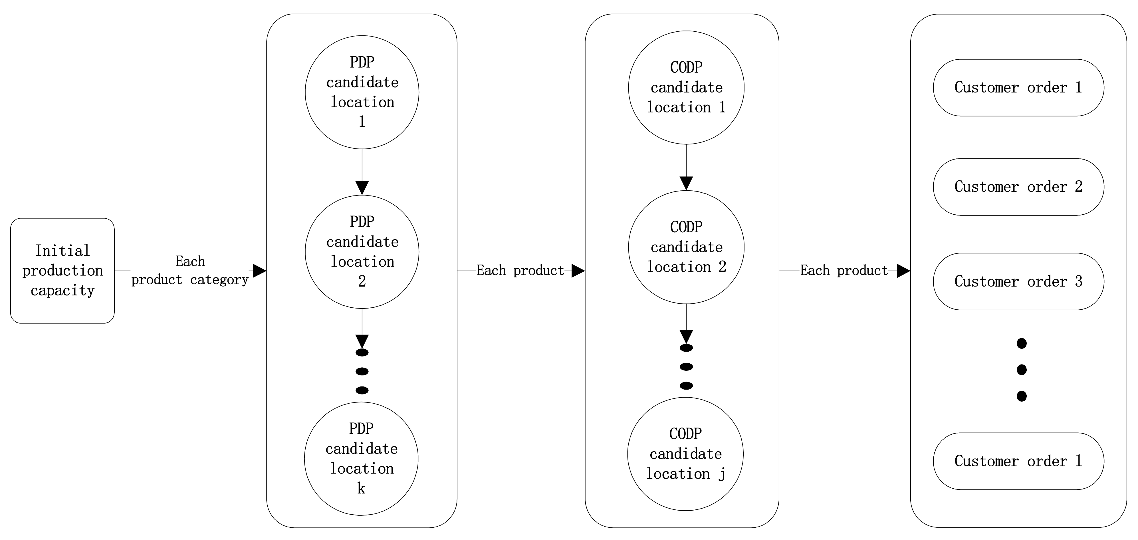
At the beginning of the cycle, the enterprise has a certain amount of initial production capacity, which should be converted into a general semi-finished product inventory for each product category and dedicated semi-finished product inventory for each product;

(2)

Among the two categories of product inventory, the storage location of general semi-finished products corresponds to PDP; that is, to select an optimal location as a PDP from multiple PDP candidate locations in the general production process of the product category for general semi-finished product storage. The storage location of the dedicated semi-finished products corresponds to CODP; that is, to select an optimal position as a CODP from multiple CODP candidate locations in the specific production process for dedicated semi-finished product storage. When the locations of PDP and CODP are determined, the production process only stays at the location of PDP or CODP;

(3)

In addition, each product corresponds to multiple customer orders. Enterprises should first use the dedicated semi-finished product inventory of this product for production according to customer order requirements. If the dedicated semi-finished product inventory is insufficient, a general semi-finished product inventory of the product category shall be used.

3.2. Problem Analysis

The study of this paper belongs to the optimization of production mode, which usually needs to consider the holding cost, delay penalty cost, etc. [46,47,48]. In addition, since the semi-finished product inventory of iron and steel enterprises will generate transportation costs and heating energy consumption when it enters the production process again, it is usually converted into the return cost. Therefore, this paper also considers the effects of holding cost, return cost and delayed production cost, with the sum of the three costs as the total costs. In addition, enterprises need to maintain a certain level of customer service to maintain stable customer relationships, so this paper also considers the impact of customer service levels.

The theoretical basis of this paper is the literature about PDP positioning and CODP positioning. In addition, according to the actual problems faced by enterprises and the content of literature research. In the initial stage of the research, we built a linear model, only considering PDP location and CODP location. However, with the deepening of the research by communication with enterprises, we found the influence of semi-finished product inventory should also be considered. Thus, the decision variables of the model were multiplied and the model became a nonlinear model. Although the linear model is clear and simple, it cannot fully reflect the research problems, so, the problem studied in this paper can be briefly described as follows: considering PDP location, CODP location and semi-finished product inventory allocation, and under the premise of satisfying specific customer service level, a nonlinear mixed integer programming model is constructed with the goal of minimizing total costs. The objectives, constraints and decision-making content of the model constructed in this paper are as follows:

The purpose of modeling in this paper is to determine the optimal locations of PDP and CODP, and the optimal semi-finished product inventory to minimize total costs. The constraints are that the customer service level achieved by production is not lower than the minimum standard of the enterprise, and that the semi-finished product inventory cannot exceed the inventory limits:

(1)

Minimizing total costs (C = C_h + C_r + C_d) is the purpose of modeling. The total costs include three aspects: first, the holding costs (C_h), which includes the holding cost of semi-finished products before participating in production and that of semi-finished products that are not involved in production; second, the return costs (C_r), namely, the cost of transportation, processing or loading and unloading when the semi-finished product is entering the production link again; and third, the delayed costs (C_d). Given the different storage locations and stocks of semi-finished products, when there is a delay in the fulfillment of customer orders delayed penalty costs are incurred;

(2)

The main constraint of modeling is that the average customer order fulfillment rate (R_pr) of all products of the enterprise is higher than the minimum customer service level (R_sl) specified by the enterprise. During the research period, the customer order information for different products is different, including order quantity, production start time, final delivery date and delayed penalty coefficient. For a certain product order, production cannot be carried out before the start time specified in the order and production must be completed before the final delivery date specified, which is known as order fulfillment. In addition, the inventory limits of semi-finished products at the locations of PDP and CODP are also important constraints;

(3)

The decision making of the model is the locations of PDP and CODP, where the semi-finished product inventory corresponds to PDP and CODP.

The locations of PDP and CODP affect total costs and production time. The production process of the Postponement is shown in Figure 1, and the parameters and customer order information in each link are shown in

Table A1. The costs and production time of the PDP candidate locations of different products.

Product Categories	PDP Candidate Location 1		PDP Candidate Location 2		PDP Candidate Location 3		PDP Candidate Location 4		PDP Candidate Location 5
First product category	Holding cost coefficient per unit	1.80	Holding cost coefficient per unit	1.89	Holding cost coefficient per unit	1.98	Holding cost coefficient per unit	2.07	Holding cost coefficient per unit	2.16
	Return cost per unit	67.00	Return cost per unit	65.50	Return cost per unit	64.00	Return cost per unit	62.50	Return cost per unit	61.00
	Time needed to produce the first kind of products in this category	25.00	Time needed to produce the first kind of products in this category	23.50	Time needed to produce the first kind of products in this category	22.00	Time needed to produce the first kind of products in this category	20.50	Time needed to produce the first kind of products in this category	19.00
	Time needed to produce the second kind of products in this category	23.00	Time needed to produce the second kind of products in this category	21.50	Time needed to produce the second kind of products in this category	20.00	Time needed to produce the second kind of products in this category	18.50	Time needed to produce the second kind of products in this category	17.00
	Time needed to produce the third kind of products in this category	21.00	Time needed to produce the third kind of products in this category	19.50	Time needed to produce the third kind of products in this category	18.00	Time needed to produce the third kind of products in this category	16.50	Time needed to produce the third kind of products in this category	15.00
Second product category	Holding cost coefficient per unit	1.37	Holding cost coefficient per unit	1.44	Holding cost coefficient per unit	1.51	Holding cost coefficient per unit	1.58	Holding cost coefficient per unit	1.65
	Return cost per unit	62.00	Return cost per unit	60.60	Return cost per unit	59.20	Return cost per unit	57.80	Return cost per unit	56.40
	Time needed to produce the first kind of products in this category	23.00	Time needed to produce the first kind of products in this category	21.00	Time needed to produce the first kind of products in this category	19.00	Time needed to produce the first kind of products in this category	17.00	Time needed to produce the first kind of products in this category	15.00
	Time needed to produce the second kind of products in this category	21.00	Time needed to produce the second kind of products in this category	19.00	Time needed to produce the second kind of products in this category	17.00	Time needed to produce the second kind of products in this category	15.00	Time needed to produce the second kind of products in this category	13.00
	Time needed to produce the third kind of products in this category	19.00	Time needed to produce the third kind of products in this category	17.00	Time needed to produce the third kind of products in this category	15.00	Time needed to produce the third kind of products in this category	13.00	Time needed to produce the third kind of products in this category	11.00
Third product category	Holding cost coefficient per unit	1.22	Holding cost coefficient per unit	1.28	Holding cost coefficient per unit	1.34	Holding cost coefficient per unit	1.40	Holding cost coefficient per unit	1.46
	Return cost per unit	68.00	Return cost per unit	66.50	Return cost per unit	65.00	Return cost per unit	63.50	Return cost per unit	62.00
	Time needed to produce the first kind of products in this category	21.00	Time needed to produce the first kind of products in this category	18.50	Time needed to produce the first kind of products in this category	16.00	Time needed to produce the first kind of products in this category	13.50	Time needed to produce the first kind of products in this category	11.00
	Time needed to produce the second kind of products in this category	19.00	Time needed to produce the second kind of products in this category	16.50	Time needed to produce the second kind of products in this category	14.00	Time needed to produce the second kind of products in this category	11.50	Time needed to produce the second kind of products in this category	9.00
	Time needed to produce the third kind of products in this category	18.00	Time needed to produce the third kind of products in this category	15.50	Time needed to produce the third kind of products in this category	13.00	Time needed to produce the third kind of products in this category	10.50	Time needed to produce the third kind of products in this category	8.00

,

Table A2. The costs and production time of the CODP candidate locations of different products.

Product Types	CODP Candidate Location 1		CODP Candidate Location 2		CODP Candidate Location 3		CODP Candidate Location 4		CODP Candidate Location 5		CODP Candidate Location 6
First kind of products in the first product category	Holding cost coefficient per unit	2.50	Holding cost coefficient per unit	2.55	Holding cost coefficient per unit	2.60	Holding cost coefficient per unit	2.65	Holding cost coefficient per unit	2.70	Holding cost coefficient per unit	2.75
	Return cost per unit	40.00	Return cost per unit	39.50	Return cost per unit	39.00	Return cost per unit	38.50	Return cost per unit	38.00	Return cost per unit	37.50
	Time needed to produce this product	16.00	Time needed to produce this product	14.00	Time needed to produce this product	12.00	Time needed to produce this product	10.00	Time needed to produce this product	8.00	Time needed to produce this product	6.00
Second kind of products in the first product category	Holding cost coefficient per unit	2.40	Holding cost coefficient per unit	2.44	Holding cost coefficient per unit	2.48	Holding cost coefficient per unit	2.52	Holding cost coefficient per unit	2.56	Holding cost coefficient per unit	2.60
	Return cost per unit	38.00	Return cost per unit	37.60	Return cost per unit	37.20	Return cost per unit	36.80	Return cost per unit	36.40	Return cost per unit	36.00
	Time needed to produce this product	14.00	Time needed to produce this product	12.00	Time needed to produce this product	10.00	Time needed to produce this product	8.00	Time needed to produce this product	6.00	Time needed to produce this product	4.00
Third kind of products in the first product category	Holding cost coefficient per unit	2.30	Holding cost coefficient per unit	2.33	Holding cost coefficient per unit	2.36	Holding cost coefficient per unit	2.39	Holding cost coefficient per unit	2.42	Holding cost coefficient per unit	2.45
	Return cost per unit	36.00	Return cost per unit	35.70	Return cost per unit	35.40	Return cost per unit	35.10	Return cost per unit	34.80	Return cost per unit	34.50
	Time needed to produce this product	12.00	Time needed to produce this product	10.00	Time needed to produce this product	8.00	Time needed to produce this product	6.00	Time needed to produce this product	4.00	Time needed to produce this product	2.00
First kind of products in the second product category	Holding cost coefficient per unit	2.10	Holding cost coefficient per unit	2.14	Holding cost coefficient per unit	2.18	Holding cost coefficient per unit	2.22	Holding cost coefficient per unit	2.26	Holding cost coefficient per unit	2.30
	Return cost per unit	38.00	Return cost per unit	37.50	Return cost per unit	37.00	Return cost per unit	36.50	Return cost per unit	36.00	Return cost per unit	35.50
	Time needed to produce this product	13.00	Time needed to produce this product	11.00	Time needed to produce this product	9.00	Time needed to produce this product	7.00	Time needed to produce this product	5.00	Time needed to produce this product	3.00
Second kind of products in the second product category	Holding cost coefficient per unit	2.00	Holding cost coefficient per unit	2.03	Holding cost coefficient per unit	2.06	Holding cost coefficient per unit	2.09	Holding cost coefficient per unit	2.12	Holding cost coefficient per unit	2.15
	Return cost per unit	36.00	Return cost per unit	35.60	Return cost per unit	35.20	Return cost per unit	34.80	Return cost per unit	34.40	Return cost per unit	34.00
	Time needed to produce this product	11.00	Time needed to produce this product	10.00	Time needed to produce this product	9.00	Time needed to produce this product	8.00	Time needed to produce this product	7.00	Time needed to produce this product	6.00
Third kind of products in the second product category	Holding cost coefficient per unit	1.90	Holding cost coefficient per unit	1.90	Holding cost coefficient per unit	1.90	Holding cost coefficient per unit	1.90	Holding cost coefficient per unit	1.90	Holding cost coefficient per unit	1.90
	Return cost per unit	34.00	Return cost per unit	34.00	Return cost per unit	34.00	Return cost per unit	34.00	Return cost per unit	34.00	Return cost per unit	34.00
	Time needed to produce this product	9.00	Time needed to produce this product	9.00	Time needed to produce this product	9.00	Time needed to produce this product	9.00	Time needed to produce this product	9.00	Time needed to produce this product	9.00
First kind of products in the third product category	Holding cost coefficient per unit	1.74	Holding cost coefficient per unit	1.77	Holding cost coefficient per unit	1.80	Holding cost coefficient per unit	1.83	Holding cost coefficient per unit	1.86	Holding cost coefficient per unit	1.89
	Return cost per unit	36.00	Return cost per unit	35.50	Return cost per unit	35.00	Return cost per unit	34.50	Return cost per unit	34.00	Return cost per unit	33.50
	Time needed to produce this product	9.00	Time needed to produce this product	8.00	Time needed to produce this product	7.00	Time needed to produce this product	6.00	Time needed to produce this product	5.00	Time needed to produce this product	4.00
Second kind of products in the third product category	Holding cost coefficient per unit	1.64	Holding cost coefficient per unit	1.66	Holding cost coefficient per unit	1.68	Holding cost coefficient per unit	1.70	Holding cost coefficient per unit	1.72	Holding cost coefficient per unit	1.74
	Return cost per unit	34.00	Return cost per unit	33.60	Return cost per unit	33.20	Return cost per unit	32.80	Return cost per unit	32.40	Return cost per unit	32.00
	Time needed to produce this product	7.00	Time needed to produce this product	6.00	Time needed to produce this product	5.00	Time needed to produce this product	4.00	Time needed to produce this product	3.00	Time needed to produce this product	2.00
Third kind of products in the third product category	Holding cost coefficient per unit	1.54	Holding cost coefficient per unit	1.55	Holding cost coefficient per unit	1.56	Holding cost coefficient per unit	1.57	Holding cost coefficient per unit	1.58	Holding cost coefficient per unit	1.59
	Return cost per unit	32.00	Return cost per unit	31.70	Return cost per unit	31.40	Return cost per unit	31.10	Return cost per unit	30.80	Return cost per unit	30.50
	Time needed to produce this product	6.00	Time needed to produce this product	5.00	Time needed to produce this product	4.00	Time needed to produce this product	3.00	Time needed to produce this product	2.00	Time needed to produce this product	1.00

and

Table A3. The order information of different products.

Product Orders	Customer Order Number	Customer Order Quantity	Customer Order Start Production Time	Final Delivery Date	Order Delayed Penalty Coefficient
First product order in the first product category	1	1000	1	10	0.1
	2	1000	1	10	0.1
	3	1000	5	20	0.1
	4	1000	10	27	0.1
Second product order in the first product category	1	1000	11	15	0.1
	2	1000	11	15	0.1
	3	1000	20	25	0.1
	4	1000	25	30	0.1
Third product order in the first product category	1	1000	5	15	0.1
	2	1000	10	20	0.1
	3	1000	15	25	0.1
	4	1000	19	30	0.1
First product order in the second product category	1	1000	1	10	0.08
	2	1000	7	15	0.08
	3	1000	7	15	0.08
	4	1000	15	28	0.08
Second product order in the second product category	1	1000	5	10	0.08
	2	1000	7	15	0.08
	3	1000	10	20	0.08
	4	1000	15	25	0.08
Third product order in the second product category	1	1000	5	10	0.08
	2	1000	10	15	0.08
	3	1000	17	25	0.08
	4	1000	22	30	0.08
First product order in the third product category	1	1000	5	10	0.06
	2	1000	5	15	0.06
	3	1000	5	15	0.06
	4	1000	7	25	0.06
Second product order in the third product category	1	1000	7	15	0.06
	2	1000	7	15	0.06
	3	1000	10	20	0.06
	4	1000	15	30	0.06
Third product order in the third product category	1	1000	10	15	0.06
	2	1000	15	25	0.06
	3	1000	15	25	0.06
	4	1000	15	30	0.06

. According to the production process, related parameters, and total costs, when the location of PDP moves to the direction of production start the holding cost per unit decreases, the return costs per unit increases, while the production time to complete the same product increases, and vice versa. Similarly, when the location of CODP is moved to the direction of the production start, the holding costs per unit decrease, the return costs per unit increase, and the production time to complete this kind of products increases.

The semi-finished product inventory corresponding to CODP and PDP will affect the total costs and customer order fulfillment time. According to the production rules, a semi-finished product inventory corresponding to CODP should be used for production first. If the semi-finished product inventory corresponding to CODP is big enough to meet the customer demand, there is no need to use the semi-finished product inventory corresponding to PDP of this product category for production. Otherwise, the unfulfilled customer orders shall be met using the semi-finished product inventory corresponding to PDP of this product category to complete subsequent production. If the semi-finished product inventory corresponding to PDP is high, it can quickly fulfill customer orders to avoid or reduce delayed penalty costs, but the holding costs will increase; if the semi-finished product inventory corresponding to CODP is low, the holding costs will decrease and the customer orders may not be able to be fulfilled, resulting in higher delayed penalty costs. In addition, the semi-finished product inventory allocation corresponding to PDP will affect the size of the holding costs.

According to the production process and features of Postponement, the above analysis is converted to an operation research model for quantitative research. Relevant parameters, decision variables, modular forms and descriptions are as follows:

3.3. Symbol Descriptions

(1)

Parameter Setting

Parameters	Parameter Meanings
$T_s$	cycle start time
$T_e$	cycle end time
$M$	total number of product categories
$m$	$m$th Product category
$N^m$	total number of product varieties in $m$th product category
$n^m$	product$n$ in $m$th product category
$L^{mn}$	total number of customer orders in product$n^m$
$l^{mn}$	No.$l$ customer order in product$n^m$
$Q^{lmn}$	number of orders of customer order $l^{mn}$
$K^m$	total number of PDP candidate locations in $m$th product category
$k^m$	PDP candidate locations of $k$ in $m$th product category
$Q^{km}$	corresponding general semi-finished product inventory when $k$ candidate location is selected in $m$th product category as PDP
$J^{mn}$	total number of CODP candidate locations in $n^m$ product
$j^{mn}$	CODP candidate locations of $j$ in $n^m$ product
$Q^{jmn}$	corresponding dedicated semi-finished product inventory when selecting $j^{mn}$ candidate location in $n^m$ product as CODP
$C_h$	cycle total holding cost
$C_h^{km}$	holding cost coefficient per unit of corresponding general semi-finished product inventory when $k^m$ candidate location is selected in $m$th product category as PDP
$C_h^{jmn}$	holding cost coefficient per unit of corresponding dedicated semi-finished product inventory when $j^{mn}$ candidate location is selected in $n^m$ product as CODP
$C_r$	cycle total return costs
$C_r^{km}$	return costs per unit of corresponding general semi-finished product inventory when $k^m$ candidate location is selected in $m$th product category as PDP
$C_r^{jmn}$	return costs per unit of corresponding dedicated semi-finished product inventory when $j^{mn}$ candidate location is selected in $n^m$ product as CODP
$C_d$	cycle total delayed penalty costs
$C_d^{km}$	delayed penalty costs per unit of corresponding general semi-finished product inventory when $k^m$ candidate location is selected in $m$th product category as PDP
$C_r^{jmn}$	delayed penalty costs per unit of corresponding general semi-finished product inventory when $k^m$ candidate location is selected in $m$th product category as PDP
$C$	cycle total costs, $C=C_h+C_r+C_d$
$P(j^{mn}$,$Q^{jmn}$)	when $j^{mn}$ candidate location is selected as the CODP in $n^m$ product, and the stock of the dedicated semi-finished product corresponding to this CODP is $Q^{jmn}$, the first $P(j^{mn}$,$Q^{jmn}$) customer orders require the dedicated semi-finished product stock corresponding to the CODP for production; the $P(j^{mn}$,$Q^{jmn}$)+1 to the $L^{mn}$ customer orders require the general semi-finished product inventory corresponding to the PDP category of this product for production
${\theta }^{lmn}$	the delayed costs coefficient in $l$ customer order in. $n^m$ product
$R_{sl}$	the lowest customer service level required, i.e., the average on-time fulfillment rate of all customer orders
$R_{pr}$	the average on-time fulfillment rate of customer orders in all products of the enterprise
$D_s^{lmn}$	the start time of $l^{mn}$ customer order
$D_e^{lmn}$	the end time of $l^{mn}$ customer order
$D_{dl}^{lmn}$	$\mathrm{the} \mathrm{final} \mathrm{delivery} \mathrm{date} \mathrm{of} l^{mn}$ customer order
$T_i^{lmn}$	the time needed to produce $l^{mn}$ customer order
$T(k^m$,$l^{mn}$)	the time needed for production from $k^m$ PDP to the fulfillment of $l^{mn}$ customer order
$U(k^m$,$l^{mn}$)	whether production can be completed before the date required by the customer order from $k^m$ PDP to the fulfillment of $l^{mn}$ customer order. 0 refers to on-time fulfillment, while 1 failure of on-time fulfillment
$T(j^{mn}$,$l^{mn}$)	the time needed for production from $j^{mn}$ CODP to the fulfillment of $l^{mn}$ customer order
$V(j^{mn}$,$l^{mn}$)	whether the production can be completed before the date required by the customer order from $j^{mn}$ CODP to the fulfillment of $l^{mn}$ customer order. 0 refers to on-time fulfillment, while 1 failure of on-time fulfillment

(2)

Decision Variables

Parameters	Parameter Meanings
$X^{km}$	whether to choose $k^m$ as PDP in $m$th product category. 1 refers to Yes, while 0 is No
$Q^{km}$	corresponding general semi-finished product inventory when $k^m$ candidate location is selected in $m$ product category as PDP
$Y^{jmn}$	whether to choose $j^{mn}$ as CODP in $n^m$ product. 1 refers to Yes, while 0 is No
$Q^{jmn}$	corresponding dedicated semi-finished product inventory when $j^{mn}$ candidate location is selected in $n^m$ product as CODP

3.4. Modeling

(1)

Objective Function

$$\begin{gathered} \mathrm{MinZ}=\mathrm{C}={\mathrm{C}}_{\mathrm{h}}+{\mathrm{C}}_{\mathrm{r}}+{\mathrm{C}}_{\mathrm{d}} \\ \begin{array}{cc}\hfill & {\mathrm{C}}_{\mathrm{h}}=\sum _{\mathrm{m}=1}^{\mathrm{M}}\left(\sum _{{\mathrm{n}}^{\mathrm{m}}=1}^{{\mathrm{N}}^{\mathrm{m}}}\left(\sum _{{\mathrm{j}}^{\mathrm{mn}}=1}^{{\mathrm{J}}^{\mathrm{mn}}}\left({\mathrm{Y}}^{\mathrm{jmn}}*{\mathrm{C}}_{\mathrm{h}}^{\mathrm{jmn}}*\sum _{{\mathrm{l}}^{\mathrm{mn}}=1}^{\mathrm{p}({\mathrm{j}}^{\mathrm{mn}},{\mathrm{Q}}^{\mathrm{jmn}})}\left({\mathrm{D}}_{\mathrm{e}}^{\mathrm{lmn}}-{\mathrm{T}}_{\mathrm{s}}\right)*{\mathrm{Q}}^{\mathrm{lmn}}\right)\right)\right)\hfill \\ \hfill & +\sum _{\mathrm{m}=1}^{\mathrm{M}}\left(\sum _{{\mathrm{n}}^{\mathrm{m}}=1}^{{\mathrm{N}}^{\mathrm{m}}}\left(\sum _{{\mathrm{j}}^{\mathrm{mn}}=1}^{{\mathrm{J}}^{\mathrm{mn}}}\left({\mathrm{Y}}^{\mathrm{jmn}}*{\mathrm{C}}_{\mathrm{h}}^{\mathrm{jmn}}*\mathrm{T}*\left({\mathrm{Q}}^{\mathrm{jmn}}-\sum _{{\mathrm{l}}^{\mathrm{mn}}=1}^{\mathrm{p}({\mathrm{j}}^{\mathrm{mn}},{\mathrm{Q}}^{\mathrm{jmn}})}{\mathrm{Q}}^{\mathrm{lmn}}\right)\right)\right)\right)\hfill \\ \hfill & +\sum _{\mathrm{m}=1}^{\mathrm{M}}\left(\sum _{{\mathrm{n}}^{\mathrm{m}}=1}^{{\mathrm{N}}^{\mathrm{m}}}\left(\sum _{{\mathrm{k}}^{\mathrm{m}}=1}^{{\mathrm{K}}^{\mathrm{m}}}\left({\mathrm{X}}^{\mathrm{km}}*{\mathrm{C}}_{\mathrm{h}}^{\mathrm{km}}\right)*\sum _{{\mathrm{j}}^{\mathrm{mn}}=1}^{{\mathrm{J}}^{\mathrm{mn}}}\left({\mathrm{Y}}^{\mathrm{jmn}}*\left(\sum _{{\mathrm{l}}^{\mathrm{mn}}=\mathrm{p}({\mathrm{j}}^{\mathrm{mn}},{\mathrm{Q}}^{\mathrm{jmn}})+1}^{{\mathrm{L}}^{\mathrm{mn}}}\left({\mathrm{D}}_{\mathrm{e}}^{\mathrm{lmn}}-{\mathrm{T}}_{\mathrm{s}}\right)*{\mathrm{Q}}^{\mathrm{lmn}}\right)\right)\right)\right)\hfill \\ \hfill & +\sum _{\mathrm{m}=1}^{\mathrm{M}}\left(\sum _{{\mathrm{n}}^{\mathrm{m}}=1}^{{\mathrm{N}}^{\mathrm{m}}}\left(\sum _{{\mathrm{k}}^{\mathrm{m}}=1}^{{\mathrm{K}}^{\mathrm{m}}}\left({\mathrm{X}}^{\mathrm{km}}*{\mathrm{C}}_{\mathrm{h}}^{\mathrm{km}}\right)*\mathrm{T}*\sum _{{\mathrm{j}}^{\mathrm{mn}}=1}^{{\mathrm{J}}^{\mathrm{mn}}}\left({\mathrm{Y}}^{\mathrm{jmn}}*\left({\mathrm{Q}}^{\mathrm{km}}-\sum _{{\mathrm{l}}^{\mathrm{mn}}=\mathrm{p}({\mathrm{j}}^{\mathrm{mn}},{\mathrm{Q}}^{\mathrm{jmn}})+1}^{{\mathrm{L}}^{\mathrm{mn}}}{\mathrm{Q}}^{\mathrm{lmn}}\right)\right)\right)\right)\hfill \end{array} \end{gathered}$$

(1)

$$\begin{array}{l}{\mathrm{C}}_{\mathrm{r}}={\displaystyle \sum _{\mathrm{m}=1}^{\mathrm{M}}\left({\displaystyle \sum _{{\mathrm{n}}^{\mathrm{m}}=1}^{{\mathrm{N}}^{\mathrm{m}}}\left({\displaystyle \sum _{{\mathrm{j}}^{\mathrm{mn}}=1}^{{\mathrm{J}}^{\mathrm{mn}}}\left({\mathrm{Y}}^{\mathrm{jmn}}*{\mathrm{C}}_{\mathrm{r}}^{\mathrm{jmn}}*{\displaystyle \sum _{{\mathrm{l}}^{\mathrm{mn}}=1}^{\mathrm{p}({\mathrm{j}}^{\mathrm{mn}},{\mathrm{Q}}^{\mathrm{jmn}})}{\mathrm{Q}}^{\mathrm{lmn}}}\right)}\right)}\right)}\\ +{\displaystyle \sum _{\mathrm{m}=1}^{\mathrm{M}}\left({\displaystyle \sum _{{\mathrm{n}}^{\mathrm{m}}=1}^{{\mathrm{N}}^{\mathrm{m}}}\left({\displaystyle \sum _{{\mathrm{k}}^{\mathrm{m}}=1}^{{\mathrm{K}}^{\mathrm{m}}}\left({\mathrm{X}}^{\mathrm{km}}*{\mathrm{C}}_{\mathrm{r}}^{\mathrm{km}}\right)*{\displaystyle \sum _{{\mathrm{j}}^{\mathrm{mn}}=1}^{{\mathrm{J}}^{\mathrm{mn}}}\left({\mathrm{Y}}^{\mathrm{jmn}}*{\displaystyle \sum _{{\mathrm{l}}^{\mathrm{mn}}=\mathrm{p}({\mathrm{j}}^{\mathrm{mn}},{\mathrm{Q}}^{\mathrm{jmn}})+1}^{{\mathrm{L}}^{\mathrm{mn}}}{\mathrm{Q}}^{\mathrm{lmn}}}\right)}}\right)}\right)}\end{array}$$

(2)

$$\begin{array}{cc}\hfill & {\mathrm{C}}_{\mathrm{d}}=\sum _{\mathrm{m}=1}^{\mathrm{M}}\left(\sum _{{\mathrm{n}}^{\mathrm{m}}=1}^{{\mathrm{N}}^{\mathrm{m}}}\left(\sum _{{\mathrm{j}}^{\mathrm{mn}}=1}^{{\mathrm{J}}^{\mathrm{mn}}}\left({\mathrm{Y}}^{\mathrm{jmn}}*\sum _{{\mathrm{l}}^{\mathrm{mn}}=1}^{\mathrm{p}({\mathrm{j}}^{\mathrm{mn}},{\mathrm{Q}}^{\mathrm{jmn}})}{\mathrm{Q}}^{\mathrm{lmn}}*\left({\mathrm{D}}_{\mathrm{s}}^{\mathrm{lmn}}+{\mathrm{Y}}^{\mathrm{jmn}}*\mathrm{T}\left({\mathrm{j}}^{\mathrm{mn}},{\mathrm{l}}^{\mathrm{mn}}\right)-{\mathrm{D}}_{\mathrm{dl}}^{\mathrm{lmn}}\right)*{\theta }^{\mathrm{lmn}}*\mathrm{V}\left({\mathrm{j}}^{\mathrm{mn}},{\mathrm{l}}^{\mathrm{mn}}\right)\right)\right)\right)\hfill \\ \hfill & +\sum _{\mathrm{m}=1}^{\mathrm{M}}\left(\sum _{{\mathrm{n}}^{\mathrm{m}}=1}^{{\mathrm{N}}^{\mathrm{m}}}\left(\sum _{{\mathrm{j}}^{\mathrm{mn}}=1}^{{\mathrm{J}}^{\mathrm{mn}}}\left({\mathrm{Y}}^{\mathrm{jmn}}*\sum _{{\mathrm{l}}^{\mathrm{mn}}=\mathrm{p}({\mathrm{j}}^{\mathrm{mn}},{\mathrm{Q}}^{\mathrm{jmn}})+1}^{{\mathrm{L}}^{\mathrm{mn}}}{\mathrm{Q}}^{\mathrm{lmn}}*\left({\mathrm{D}}_{\mathrm{s}}^{\mathrm{lmn}}+{\mathrm{X}}^{\mathrm{km}}*\mathrm{T}\left({\mathrm{k}}^{\mathrm{m}},{\mathrm{l}}^{\mathrm{mn}}\right)-{\mathrm{D}}_{\mathrm{dl}}^{\mathrm{lmn}}\right)*{\theta }^{\mathrm{lmn}}*\sum _{{\mathrm{k}}^{\mathrm{m}}=1}^{{\mathrm{K}}^{\mathrm{m}}}\left({\mathrm{X}}^{\mathrm{km}}*\mathrm{U}\left({\mathrm{k}}^{\mathrm{m}},{\mathrm{l}}^{\mathrm{mn}}\right)\right)\right)\right)\right)\hfill \end{array}$$

(3)

Equation (1) refers to the holding costs. The holding costs consist of four parts: first, the holding costs of semi-finished product inventory incurred before being processed into finished products, when the first $p$ customer orders of a certain product are produced using the dedicated semi-finished product inventory corresponding to CODP; second, the remaining holding costs that are unable to meet the dedicated semi-finished product inventory for another complete customer order of this product, when the first $p$ customer orders of a certain kind of products are produced using the dedicated semi-finished product inventory corresponding to CODP; third, the holding costs of these semi-finished product inventories before processing, when the $p+1$ and subsequent customer orders of certain kind of products are produced using the general semi-finished product inventory corresponding to PDP; fourth, the remaining holding costs of the dedicated semi-finished product inventory after meeting the production demand of all kinds of products for the general semi-finished product inventory corresponding to PDP of a certain product category.

Equation (2) refers to the return costs, which consist of two parts: first, the return costs of the semi-finished product inventory before their use when the first $p$ customer orders of a certain kind of product are produced using the dedicated semi-finished product inventory corresponding to CODP; second, the return costs of general semi-finished product inventory before their use when the $p+1$ and subsequent customer orders of a certain kind of product are produced using the general semi-finished product inventory corresponding to PDP.

Equation (3) refers to the delayed costs. The delayed costs consist of two parts: first, when the first $p$ customer orders of a certain kind of products are produced using the dedicated semi-finished product inventory corresponding to CODP, the production is not completed before the final delivery date and delayed penalty costs are generated; second, when the $p+1$ and subsequent customer orders of a certain kind of product are produced using the general semi-finished product inventory corresponding to PDP, the production is not completed before the final delivery date, so delayed penalty costs are generated.

(2)

Constraints

$${\mathrm{Y}}^{\mathrm{jmn}}=0\mathrm{or}1$$

(4)

$${\mathrm{X}}^{\mathrm{km}}=0\mathrm{or}1$$

(5)

$${\displaystyle \sum _{{\mathrm{j}}^{\mathrm{mn}}=1}^{{\mathrm{J}}^{\mathrm{mn}}}{\mathrm{Y}}^{\mathrm{jmn}}}=1$$

(6)

$${\displaystyle \sum _{{\mathrm{k}}^{\mathrm{m}}=1}^{{\mathrm{K}}^{\mathrm{m}}}{\mathrm{X}}^{\mathrm{km}}}=1$$

(7)

$$0\le {\mathrm{Q}}^{\mathrm{jmn}}\le 5000$$

(8)

$$0\le {\mathrm{Q}}^{\mathrm{km}}\le 5000$$

(9)

$${\mathrm{when} \mathrm{Y}}^{\mathrm{jmn}}=0, {\mathrm{Q}}^{\mathrm{jmn}}=0$$

(10)

$${\mathrm{when} \mathrm{X}}^{\mathrm{km}}=0, {\mathrm{Q}}^{\mathrm{km}}=0$$

(11)

$${\mathrm{when} \mathrm{D}}_{\mathrm{dl}}^{\mathrm{lmn}}-{\mathrm{D}}_{\mathrm{s}}^{\mathrm{lmn}}-{\mathrm{Y}}^{\mathrm{jmn}}*\mathrm{T}\left({\mathrm{j}}^{\mathrm{mn}},{\mathrm{l}}^{\mathrm{mn}}\right)<0, \mathrm{V}\left({\mathrm{j}}^{\mathrm{mn}},{\mathrm{l}}^{\mathrm{mn}}\right)=1; otherwise\mathrm{V}\left({\mathrm{j}}^{\mathrm{mn}},{\mathrm{l}}^{\mathrm{mn}}\right)=0$$

(12)

$${\mathrm{when} \mathrm{D}}_{\mathrm{dl}}^{\mathrm{lmn}}-{\mathrm{D}}_{\mathrm{s}}^{\mathrm{lmn}}-{\mathrm{X}}^{\mathrm{km}}*\mathrm{T}\left({\mathrm{k}}^{\mathrm{m}},{\mathrm{l}}^{\mathrm{mn}}\right)<0, \mathrm{U}\left({\mathrm{k}}^{\mathrm{m}},{\mathrm{l}}^{\mathrm{mn}}\right)=1; otherwise\mathrm{U}\left({\mathrm{k}}^{\mathrm{m}},{\mathrm{l}}^{\mathrm{mn}}\right)=0$$

(13)

$$\mathrm{p}({\mathrm{j}}^{\mathrm{mn}},{\mathrm{Q}}^{\mathrm{jmn}})\mathrm{is} \mathrm{an} \mathrm{integer}, and{\displaystyle \sum _{{\mathrm{l}}^{\mathrm{mn}}=1}^{\mathrm{p}({\mathrm{j}}^{\mathrm{mn}},{\mathrm{Q}}^{\mathrm{jmn}})}{\mathrm{Q}}^{\mathrm{lmn}}}\le {\mathrm{Q}}^{\mathrm{jmn}}<{\displaystyle \sum _{{\mathrm{l}}^{\mathrm{mn}}=1}^{\mathrm{p}({\mathrm{j}}^{\mathrm{mn}},{\mathrm{Q}}^{\mathrm{jmn}})+1}{\mathrm{Q}}^{\mathrm{lmn}}}$$

(14)

$$\begin{array}{c}\hfill {\mathrm{R}}_{\mathrm{f}}=\sum _{\mathrm{m}=1}^{\mathrm{M}}\left(\sum _{{\mathrm{n}}^{\mathrm{m}}=1}^{{\mathrm{N}}^{\mathrm{m}}}\left(\sum _{{\mathrm{j}}^{\mathrm{mn}}=1}^{{\mathrm{J}}^{\mathrm{mn}}}\left(\frac{{\mathrm{Y}}^{\mathrm{jmn}}*{\displaystyle \sum _{{\mathrm{l}}^{\mathrm{mn}}=1}^{\mathrm{p}({\mathrm{j}}^{\mathrm{mn}},{\mathrm{Q}}^{\mathrm{jmn}})}}{\mathrm{Q}}^{\mathrm{lmn}}*\left(1-\mathrm{V}\left({\mathrm{j}}^{\mathrm{mn}},{\mathrm{l}}^{\mathrm{mn}}\right)\right)+{\mathrm{Y}}^{\mathrm{jmn}}*{\displaystyle \sum _{{\mathrm{k}}^{\mathrm{m}}=1}^{{\mathrm{K}}^{\mathrm{m}}}}\left({\mathrm{X}}^{\mathrm{km}}\right)*{\displaystyle \sum _{{\mathrm{l}}^{\mathrm{mn}}=\mathrm{p}({\mathrm{j}}^{\mathrm{mn}},{\mathrm{Q}}^{\mathrm{jmn}})+1}^{{\mathrm{L}}^{\mathrm{mn}}}}{\mathrm{Q}}^{\mathrm{lmn}}*\left(1-\mathrm{U}\left({\mathrm{k}}^{\mathrm{m}},{\mathrm{l}}^{\mathrm{mn}}\right)\right)}{{\displaystyle \sum _{{\mathrm{L}}_{\mathrm{i}}^{\mathrm{MaNb}}=1}^{{\mathrm{L}}^{\mathrm{MaNb}}}}{\mathrm{Q}}_{\mathrm{i}}^{\mathrm{MaNb}}}\right)\right)\right)\ge {\mathrm{R}}_{\mathrm{sl}}\end{array}$$

(15)

• Equation (4) indicates whether a certain kind of product chooses a certain location as CODP. 1 means Yes, while 0 means No.
• Equation (5) indicates whether a certain product category chooses a certain location as PDP. 1 means Yes, while 0 means No.
• Equation (6) indicates there is only one CODP in a certain kind of product.
• Equation (7) indicates there is only one PDP in a certain product category.
• Equation (8) indicates that the “dedicated semi-finished product inventory” corresponding to CODP of a certain kind of product cannot exceed 5000.
• Equation (9) indicates that the “general semi-finished product inventory” of a certain product category cannot exceed 5000.
• Equation (10) indicates when a certain CODP candidate location is not selected as CODP, and the corresponding dedicated semi-finished product inventory is 0.
• Equation (11) indicates when a certain PDP candidate location is not selected as PDP, and the corresponding general semi-finished product inventory is 0.
• Equation (12) indicates whether the customer order can be fulfilled on time when a certain customer order uses the “dedicated semi-finished product inventory” corresponding to CODP for production. 1 means Yes, while 0 means No.
• Equation (13) indicates whether the customer order can be fulfilled on time when a certain customer order uses the “general semi-finished product inventory” corresponding to PDP for production. 1 means Yes, while 0 means No.
• Equation (14) indicates when a certain customer order uses the dedicated semi-finished product inventory corresponding to CODP for production, its inventory can only satisfy the order quantity of the first p customer orders, and the p+1 and subsequent customer orders need to be produced using the general semi-finished product inventory corresponding to PDP.
• Equation (15) indicates the average on-time fulfillment rate of customer orders for all products in all categories, which should be greater than or equal to the minimum level as required.

4. Algorithm Design and Simulation

4.1. The Design and Comparison of Heuristic Algorithm

This paper constructs a nonlinear mixed integer programming model. It is very difficult to solve the large-scale nonlinear mixed integer programming model by using the exact algorithm. In addition, according to the relevant literature, for the mixed integer programming problem, the particle swarm algorithm is more efficient and accurate than other heuristic algorithms (tabu search algorithm, cuckoo search algorithm, enumeration algorithm, etc.), so the particle swarm algorithm is used to solve the model [39,40,41,49].

(1)

Pseudocode of Heuristic Algorithm

This paper solves the model with PSO, where the pseudocode of the principles and application of the Algorithm 1 are as follows:

Algorithm 1: The positioning of CODP and PDP and the semi-finished product inventory allocation process in Postponement

1:  function PSO(m): 2:    for Every particle do: 3:    Initialization speed 4:     Initialization location 5:    Optimal solution for the population ← Optimal objective function value in all particles 6:   end for 7:   while Number of iterations unachieved m: 8:    for Every particle do: 9:     for Every dimension i do: 10:      Speed update: vi ← ω · vi + c1 · (pbesti − xi) + c2 · (gbesti − xi) 11:      Location update: $x_i\leftarrow v_i+x_i$ 12:     Calculate the objective function value of the particle with x in the objective function 13:    end for 14:     Update of optimal solution for the population 15:   end while 16:  end function 17:  function The positioning of CODP and corresponding semi-finished product inventory allocation, the positioning of PDP and corresponding semi-finished product inventory allocation: 18:    for Every product category do: 19:     x ← (The location of CODP of the first product, the semi-finished product inventory corresponding to CODP of the first product..., the location of CODP of n product, the semi-finished product inventory corresponding to CODP of n product, the location of PDP, total customer order quantity --allocated inventory) 20:     x ← PSO 21:    The location of PDP in this category and the corresponding semi-finished product inventory, the location of CODP in this category and the corresponding semi-finished product inventory ← x 22:    end for 23:   end function 24:  function Surplus allocation: 25:   Unallocated production capacity ← Overall capacity—Total demand for customer orders 26:   while There is still unallocated production capacity: 27:    for Every location of PDP with available storage do: 28:     Unit gain ← Unit objective function gain/maximum storage capacity resulting from maximum storage capacity at this location 29:    end for 30:     The location of PDP corresponding to the minimum objective function gain per unit continues to allocate inventory 31:    Unallocated production capacity ← Unallocated production capacity—Capacity allocated on the selected location of PDP 32:   end function 33:   main 34:    Unallocated inventory ← Initial capacity 35:    Order inventory allocation 36:    Unallocated inventory ← Initial capacity—Total order quantity 37:    Surplus allocation 38:   end procedure

(2)

Comparison of Heuristic Algorithm and Exact Algorithm

Relevant literature suggests that PSO is better than other heuristic algorithms for solving mixed integer programming problems, but relevant research cannot prove PSO being accurate enough. Therefore, the mixed integer programming model built in this paper is based on a small-scale example comparing PSO with exact algorithm. The specific results are as follows:

Based on the mixed integer nonlinear programming model built in this paper, exact algorithm (achieved through lingo) and PSO (achieved through python) are used to solve and compare small-scale examples with different numbers of variables. The results are shown in

Table 2. Comparison of PSO and exact algorithm.

Model Parameter Settings	Number of Variables	The Average Difference between the Results Calculated by the Two Algorithms	Average Computation Time with Exact Algorithm	Average Computation Time Using Particle Swarm Heuristics
One product category, each product category has 2 PDP candidate locations. Each product category consists of 2 kinds of products, and each kind of product has 2 CODP candidate locations	12	0.0223%	1.1 min	8 s
One product category, each product category has 2 PDP candidate locations. Each product category consists of 2 kinds of products, and each kind of product has 3 CODP candidate locations	16	0.1391%	1.4 min	10 s
One product category, each product category has 3 PDP candidate locations. Each product category consists of 2 kinds of product, and each kind of product has 4 CODP candidate locations	22	0.4667%	3.6 min	11 s
One product category, each product category has 3 PDP candidate locations. Each product category consists of 2 kinds of product, and each kind of product has 5 CODP candidate locations	26	0.4179%	8 min	12 s
One product category, each product category has 3 PDP candidate locations. Each product category consists of 3 kinds of product, and each kind of product has 5 CODP candidate locations	36	0.6358%	3.5 h	20 s

. The mean difference between the calculation results of the two algorithms is small, and the heuristic algorithm has a faster calculating speed.

4.2. The Solution and Description of Large-Scale Examples

To verify the validity of the model, this paper uses a large iron and steel enterprise as the study object and adopts the method of simulating the market environment and production environment to conduct a case study subject, while observing the privacy requirements and research needs of the enterprise. The enterprise in the case study is a large iron and steel enterprise running well, which has three product categories: hot-rolled coils, cold-rolled coils, and tin-plated coils. Each product category includes a variety of products. Enterprises pay attention to the two objectives of minimizing inventory costs and maintaining a customer service level not lower than the market requirements. The main factors to be considered include: the holding costs, the return costs, and the delayed costs. Among them, in the investigated enterprises, the holding costs represent the various expenses consumed by enterprises to retain these stocks. The return costs represent the transportation cost and energy consumption cost that may be incurred when semi-finished products are put into production again. The delayed costs represent the compensation cost caused through the delay caused by the unreasonable distribution of semi-finished products. These three aspects comprehensively reflect the influencing factors considered by iron and steel enterprises in actual production. In this case, we consider three product categories: hot-rolled coils, cold-rolled coils, and tin-plated coils. Each product category includes five PDP candidate positions, and various parameters of each position are shown in Table A1 in the Appendix A; three products are considered for each product category, and each product includes six CODP candidate positions. The various parameters of each position are shown in Table A2 in the Appendix A. In addition, it is assumed that there are four orders for each product, and various explanations of each order are shown in Table A3 in the Appendix A. Some information is not included in the Appendix A. Specifically, the production cycle is 30 days, the initial production capacity is 60,000, the inventory capacity limit of semi-finished products corresponding to PDP and CODP is 5000, and the minimum customer service level is 0.85. At the same time, PSO can be used as a tool for case analysis in this paper. The problem is solved with the model built in this paper, with related information and results as follows:

{‘pdp’: [4000, 0, 0, 0, 0], ‘codp’: [[4000, 0, 0, 0, 0, 0], [0, 0, 4000, 0, 0, 0], [0, 4000, 0, 0, 0, 0]]}

{‘pdp’: [5000, 0, 0, 0, 0], ‘codp’: [[0, 0, 0, 4000, 0, 0], [0, 0, 0, 4000, 0, 0], [0, 4000, 0, 0, 0, 0]]}

{‘pdp’: [5000, 0, 0, 0, 0], ‘codp’: [[0, 0, 0, 0, 0, 4000], [0, 4000, 0, 0, 0, 0], [0, 0, 0, 0, 0, 4000]]}

Taking the first row of the calculation results as an example, for the first product category the optimal location of PDP is 1, and the optimal general semi-finished product inventory corresponding to PDP is 4000; for the first kind of product in the first product category, the optimal location of CODP is 1, and the optimal dedicated semi-finished product inventory corresponding to CODP is 4000; for the second kind of product in the first product category, the optimal location of CODP is 3, and the optimal dedicated semi-finished product inventory corresponding to CODP is 4000; for the third kind of product in the first product category, the optimal location of CODP is 2, and the optimal dedicated semi-finished product inventory corresponding to CODP is 4000. Other product categories and their optimal location and inventory of the included products are analogous. The total cost using the optimal decision making is 3,314,040 CNY (Chinese yuan).

5. Discussions

The model built in this paper includes multiple parameters that are all influencing factors of optimal decision making. In the above example all parameters are set, but in the actual production process they may be subject to changes, which in turn affect decision making. This paper conducts a simulation analysis based on the actual situation of the investigated enterprises, assuming that the observed period is 30 days long and the initial production capacity is 60,000 tons. The data in the Appendix A are used for discussions.

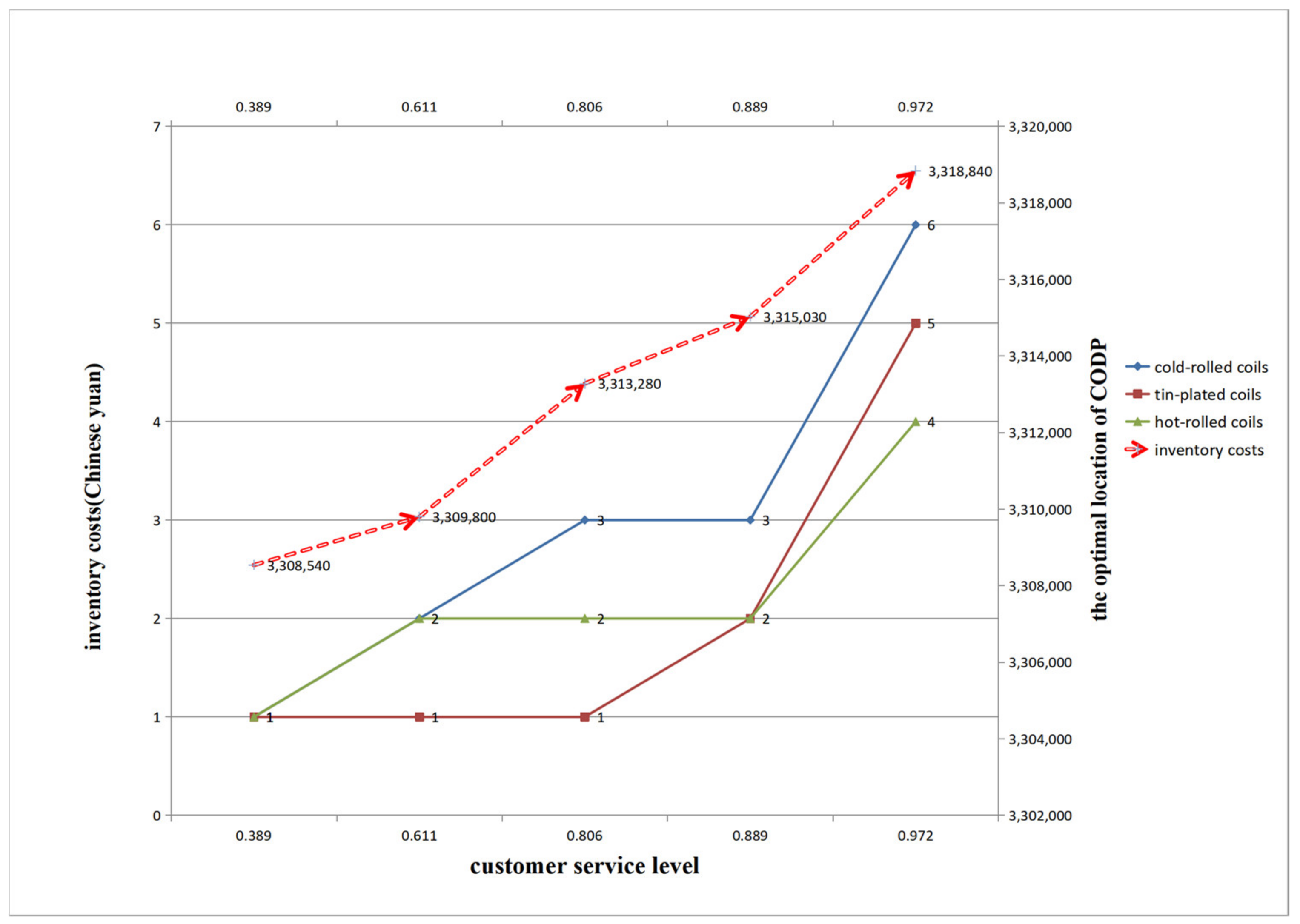
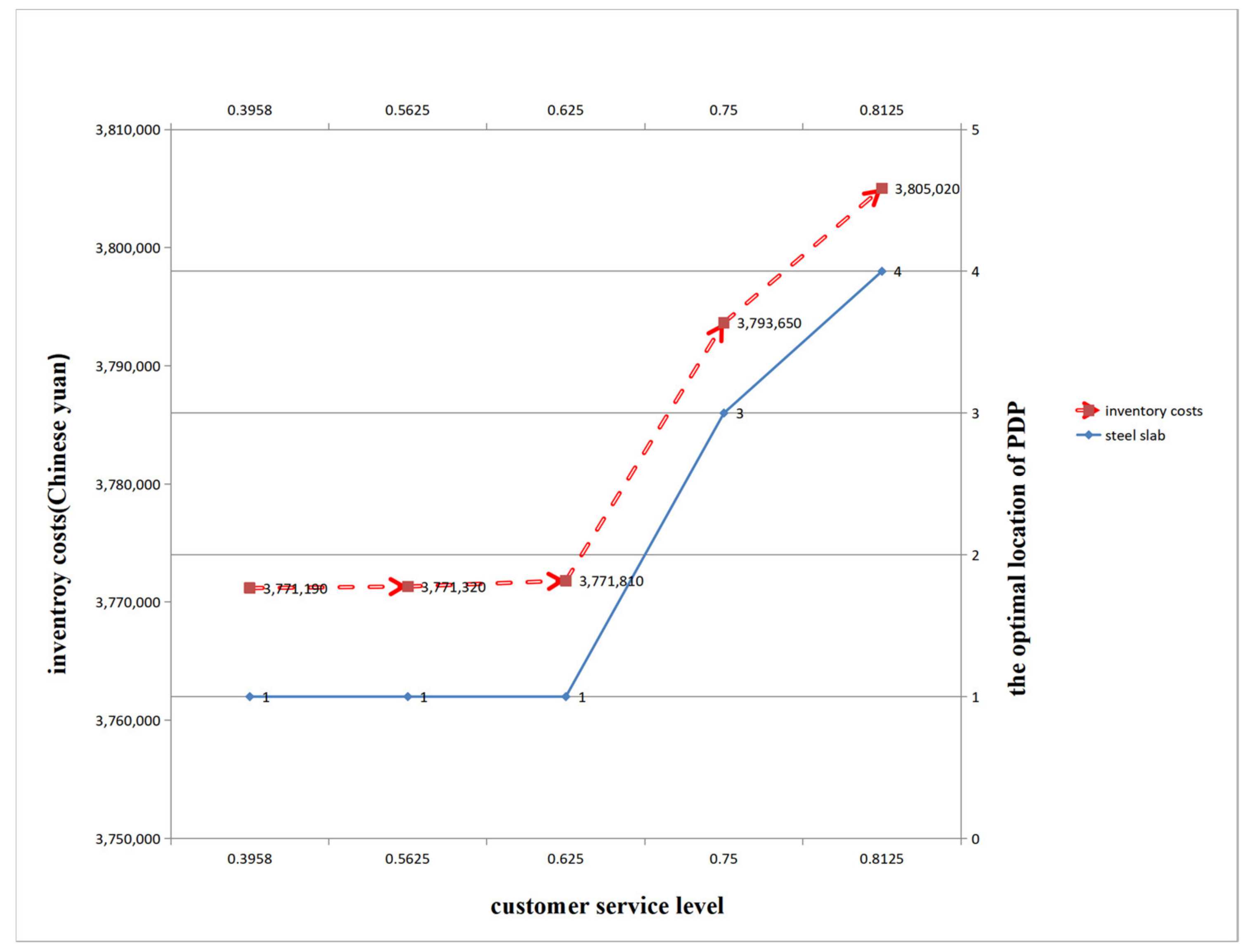
5.1. The Influence of Customer Service Level

For high-end tin-plated coils, mid-end cold-rolled coils, and low-end hot-rolled coils, other parameters are set, and the influence of customer service level on the optimal location of CODP and total costs of the three kinds of products is analyzed by changing the customer service level. Specific analysis results are shown in Figure 2:

Figure 2 shows that with the improvement of customer service level, the optimal location of CODP of the three kinds of products gradually moved from the beginning of production to the end of production, and the total costs also gradually increased. Similarly, as shown in Figure 3, the impact of the improvement of customer service level on the optimal position of PDP of steel slab is similar to that on CODP. Further studies show that in the production and operation of enterprises, and under the premise of achieving the minimum customer service level, enterprises can control their production time and total costs by adjusting the processing degree of semi-finished products. In the model of this paper, the control of the processing degree of semi-finished products is reflected in the adjustment of the optimal locations of CODP and PDP.

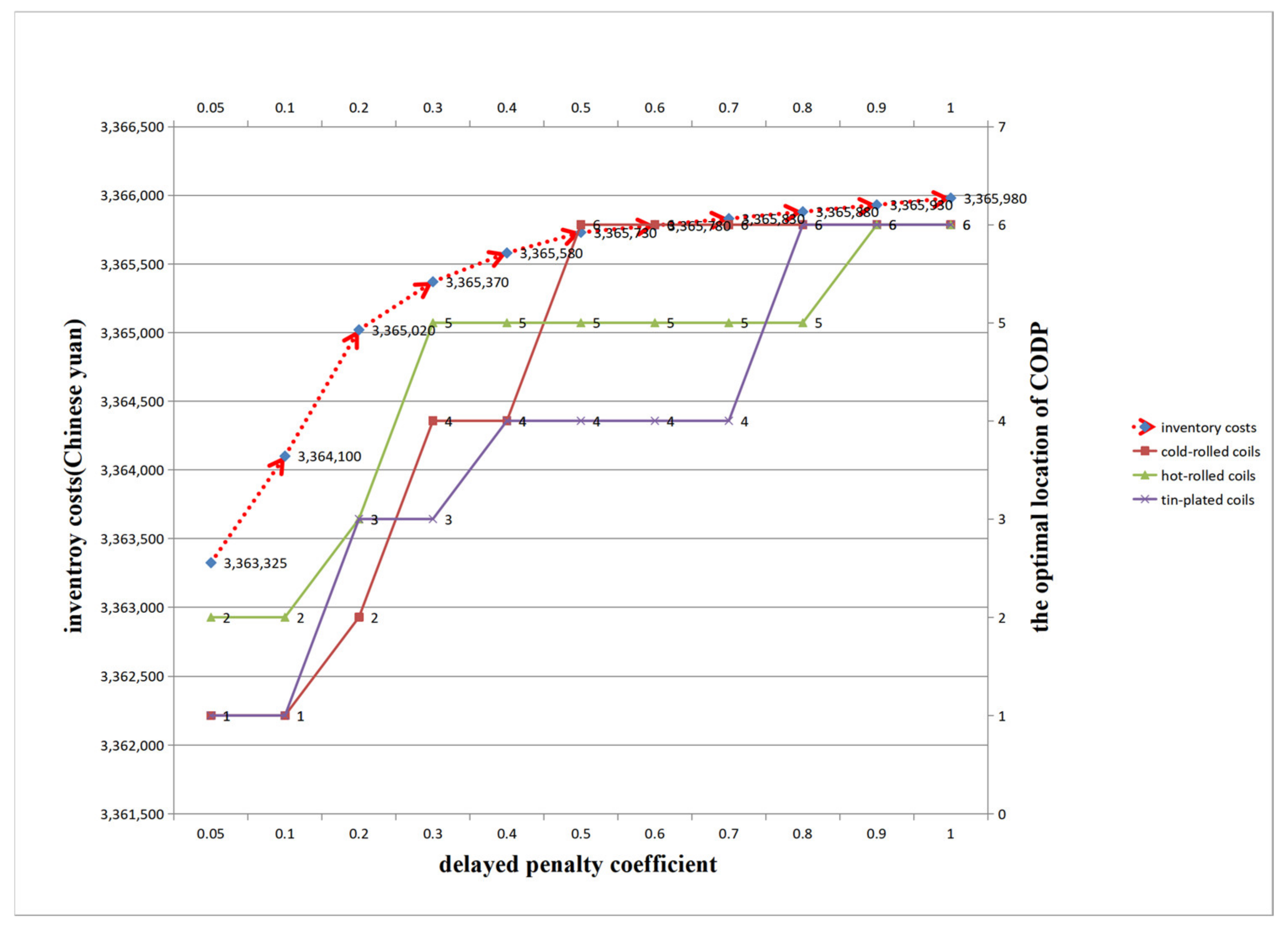
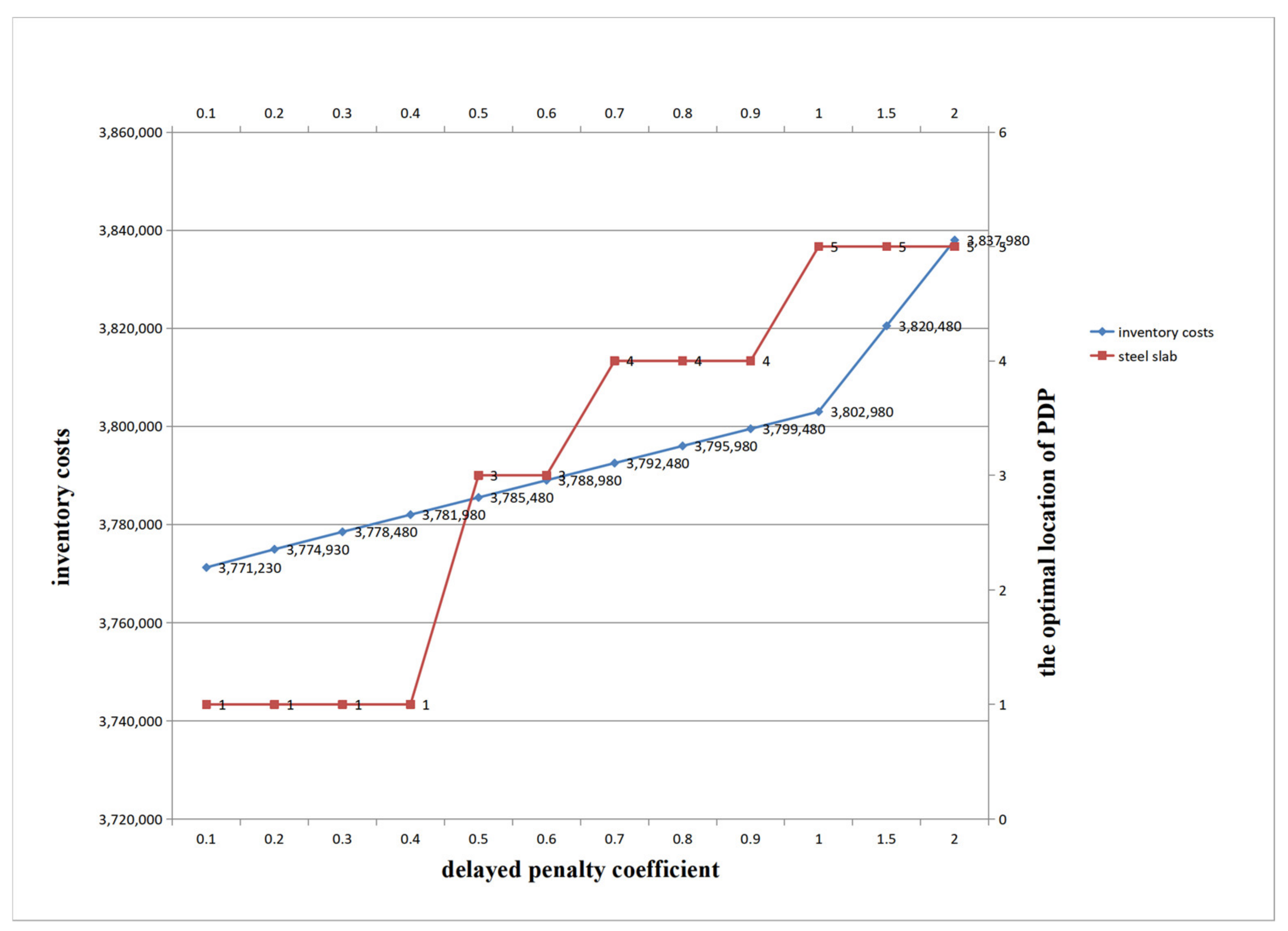
5.2. Influence of Delayed Penalty Coefficient

Other parameters are set, and the influence of the delayed penalty coefficient on the optimal location of CODP, the optimal location of PDP, and total costs of the three kinds of products is analyzed by changing the delayed penalty coefficient. The specific analysis results are shown in Figure 4 and Figure 5:

Figure 4 and Figure 5 show that the optimal location of CODP of the three kinds of products gradually moves rightward with the increase in the delayed penalty coefficient, and the total costs also gradually increase. Similarly, when PDP participates in product production corresponding to the semi-finished product inventory, the impact of delay penalty coefficient on the optimal position of PDP is similar to that on CODP. Further studies show that, in the production and operation of enterprises, delayed penalty coefficient reflects the degree of strictness of the customers on the on-time fulfillment of orders. Specifically, a delayed penalty coefficient is specified in the contract to determine the delayed cost of the enterprise, and the enterprise is urged to complete the order within the specified time, which further affects the material preparation location of semi-finished products on all levels and the total costs (to a certain extent).

5.3. Integrated Influence of Return Costs per Unit, Holding Costs per Unit and Delayed Penalty Coefficient

The holding costs per unit, return costs per unit, and delayed cost per unit of different CODP candidate locations of the three kinds of products are different. The sum of the holding costs per unit, return costs per unit, and delayed costs per unit are the total costs per unit, and the optimal location of CODP of the product will be located where the total cost per unit is the lowest. Similarly, the optimal location of PDP of the product will be located where the total costs per unit is the lowest.

5.4. Analysis of Optimal Semi-Finished Product Inventory

When the optimal locations of CODP and PDP are determined, a certain amount of dedicated semi-finished product inventory and general semi-finished product inventory will be stored in this location. The amount of semi-finished product inventory will affect the customer service level and total costs.

(1)

Optimal dedicated semi-finished product inventory corresponding to CODP

If the dedicated semi-finished product inventory corresponding to CODP has no capacity limits, or the capacity limits are greater than the total order quantity for this product, the optimal dedicated semi-finished product inventory corresponding to CODP is the total order quantity for this product; if the dedicated semi-finished product inventory corresponding to CODP has capacity limits, and the capacity limits are lower than the total order quantity for this product, the optimal semi-finished product inventory corresponding to CODP is the upper limit of the capacity.

(2)

Optimal general semi-finished product inventory corresponding to PDP

Firstly, in all determined PDPs, search for the PDP with the lowest total costs per unit, convert the available capacity into its semi-finished product inventory, and reach the capacity limit as permitted. Then, continue to search for the PDP with the next-lowest total costs per unit among other determined PDPs with unallocated capacity, and continue to convert the available capacity into its semi-finished product inventory and reach the capacity limit as permitted by the capacity limit. Finally, repeat the above steps, and continue to allocate available capacity until all available capacity is allocated.

6. Conclusions

This paper conducts a quantitative study on the optimization of the Postponement in iron and steel enterprises and comes to the following conclusions after fully considering the influence of the optimal locations of PDP and CODP and the optimal semi-finished product inventory. The study supplements the research deficiency on Postponement in the continuous manufacturing enterprises, and also enriches the content of the quantitative research on Postponement. The research results are as follows:

(1)

The optimal locations of CODP and PDP will move to the end of production with the improvement of customer service level, but not necessarily to the rightmost. The total costs also increase with the improvement of customer service level. In addition, the optimal location of PDP changes more slowly than that of CODP.

(2)

With the increase in the delayed penalty coefficient, the total costs continue to increase, and the locations of CODP and PDP gradually move to the end of production and finally to the far right.

(3)

When the return costs per unit, holding costs per unit, and delayed penalty coefficient change at the same time, the three influencing factors can be converted into the total costs per unit, the size of which affects the change of the optimal locations of CODP and PDP.

(4)

The size of the inventory capacity of dedicated semi-finished products corresponding to CODP directly affects whether the semi-finished product inventory corresponding to PDP participates in production, which in turn affects the optimal semi-finished product inventory at all levels.

The essential problem of this paper is the quantitative modeling of Postponement in continuous enterprises, which can be applied to all similar continuous manufacturing enterprises, such as the glass manufacturing industry, oil refining and processing industry, food manufacturing industry, etc. The model constructed in this paper can effectively guide the control of Postponement in these enterprises. This paper expands the content of the optimization of the Postponement in continuous manufacturing enterprises. However, the research in the paper has limitations, mainly including two aspects: first, when building the model, the factors considered are internal factors of the enterprise, and the factors selected are based on production experience and financial indicators, without considering the impact of external factors of the enterprise; second, when building the model, this paper only considers the single-cycle production situation and does not consider the construction of Postponement in the multiple-cycles situation. Future studies can be carried out in two aspects: first, we can use data mining methods or statistical analysis methods to analyze the internal and external factors that affect Postponement, and further optimize the model; secondly, considering the situation of different continuous manufacturing enterprises, the optimization problem of Postponement should be studied in multiple cycles.

References

1. Ono, A.; Kubo, T. What determines firms’ intention to postpone product differentiation? J. Mark. Channels 2018, 25, 198–210. [Google Scholar] [CrossRef]
2. Xu, D.; Liu, E.; Duan, W.; Yang, K. Consumption-Driven Carbon Emission Reduction Path and Simulation Research in Steel Industry: A Case Study of China. Sustainability 2022, 14, 13693. [Google Scholar] [CrossRef]
3. Fransoo, J.C.; Rutten, W.G.M.M. A typology of production control situations in process industries. Int. J. Oper. Prod. Manag. 1994, 14, 47–57. [Google Scholar] [CrossRef] [Green Version]
4. Denton, B.; Gupta, D.; Jawahir, K. Managing increasing product variety at integrated steel mills. Interfaces 2003, 33, 41–53. [Google Scholar] [CrossRef]
5. Rocha, F.; Silva, E.; Lopes, Â.; Dias, L.; Pereira, G.; Fernandes, N.O.; Carmo-Silva, S. Materials Flow Control in Hybrid Make-to-Stock/Make-to-Order Manufacturing. In International Conference on Computational Logistics; Springer: Cham, Switzerland, 2015; pp. 559–568. [Google Scholar]
6. Fernandes, N.; Silva, C.; Carmo-Silva, S. Order release in a hybrid MTO-MTS two-stage production system. In Proceedings of the Pre-prints of the 18th International Working Seminar on Production Economics, Innsbruck, Austria, 24–28 February 2014. [Google Scholar]
7. Liu, Q.Q. A Case Study of Hybrid MTS-MTO Production System in Age. Ph.D. Thesis, Beijing University of Technology, Beijing, China, 2016. [Google Scholar]
8. Rossit, D.A.; Tohmé, F.; Frutos, M. Production planning and scheduling in Cyber-Physical Production Systems: A review. Int. J. Comput. Integr. Manuf. 2019, 32, 385–395. [Google Scholar] [CrossRef]
9. Cannas, V.G.; Pero, M.; Rossi, T.; Gosling, J. Integrate Customer Order Decoupling Point and Mass Customisation Concepts: A Literature Review. In Customization 4.0. Springer Proceedings in Business and Economics; Springer: Cham, Switzerland, 2018. [Google Scholar]
10. Fries, C.; Bauernhansl, T.; Planning, C. Customer-Induced Planning Deviations within Order Management. Procedia Comput. Sci. 2022, 200, 71–82. [Google Scholar] [CrossRef]
11. Cantini, A.; Peron, M.; De Carlo, F.; Sgarbossa, F. A decision support system for configuring spare parts supply chains considering different manufacturing technologies. Int. J. Prod. Res. 2022, 1–21. [Google Scholar] [CrossRef]
12. Guo, L.; Chen, S.; Allen, J.K.; Mistree, F. A Framework for Designing the Customer-Order Decoupling Point to Facilitate Mass Customization. J. Mech. Des. 2021, 143, 022002. [Google Scholar] [CrossRef]
13. Ferreira, K.A.; Flávio, L.A.; Rodrigues, L.F. Postponement: Bibliometric analysis and systematic review of the literature. Int. J. Logist. Syst. Manag. 2018, 30, 69–94. [Google Scholar] [CrossRef]
14. Wikner, J.; Noroozi, S. A modularised typology for flow design based on decoupling points -a holistic view on process industries and discrete manufacturing industries. Prod. Plan. Control. 2016, 27, 1344–1355. [Google Scholar] [CrossRef]
15. Buergin, J.; Belkadi, F.; Hupays, C.; Gupta, R.K.; Bitte, F.; Lanza, G.; Bernard, A. A modular-based approach for Just-In-Time Specification of customer orders in the aircraft manufacturing industry. CIRP J. Manuf. Sci. Technol. 2018, 21, 61–74. [Google Scholar] [CrossRef]
16. Giesberts, P.M.J.; Van Der Tang, L. Dynamics of the customer order decoupling point: Impact on information systems for production control. Prod. Plan. Control. Manag. Oper. 1992, 3, 300–313. [Google Scholar] [CrossRef] [Green Version]
17. Daaboul, J.; da Cunha, C.; le Duigou, J.; Novak, B.; Bernard, A. Differentiation and customer decoupling points: An integrated design approach for mass customization. Concurr. Eng. 2015, 23, 284–295. [Google Scholar] [CrossRef]
18. Immawan, T.; Arkeman, Y. Sustainable supply chain management for Make To Stock-Make To Order production typology case study: Batik industry in Solo Indonesia. Supply Chain. Manag. 2015, 7, 94–106. [Google Scholar]
19. Ji, J.H.; Qi, L.L.; Gu, Q.L. Study on CODP position of process industry implemented mass customization. Syst. Eng.-Theory Pract. 2007, 27, 151–157. [Google Scholar] [CrossRef]
20. Zandieh, M.; Motallebi, S. Determination of production planning policies for different products in process industries: Using discrete event simulation. Prod. Eng. 2018, 12, 737–746. [Google Scholar] [CrossRef]
21. Kitayama, S.; Yasuda, K. A method for mixed integer programming problems by particle swarm optimization. Electr. Eng. Jpn. 2006, 152, 813–820. [Google Scholar]
22. Şahin, M.; Kellegöz, T. A new mixed-integer linear programming formulation and particle swarm optimization based hybrid heuristic for the problem of resource investment and balancing of the assembly line with multi-manned workstations. Comput. Ind. Eng. 2019, 133, 107–120. [Google Scholar] [CrossRef]
23. Ramón-Lumbierres, D.; Cervera, F.J.H.; Minguella-Canela, J.; Muguruza-Blanco, A. Optimal postponement in supply chain network design under uncertainty: An application for additive manufacturing. Int. J. Prod. Res. 2021, 59, 5198–5215. [Google Scholar] [CrossRef]
24. Wang, Y.; Chen, Y. Multi-CODP adjustment model and algorithm driven by customer requirements in dynamic environments. Clust. Comput. 2016, 19, 2119–2131. [Google Scholar] [CrossRef]
25. Qian, H. Research on Customer Order Decoupling Point Based on Adjustable Machining Operations. Master’s Thesis, Hefei University of Technology, Hefei, China, 2016. [Google Scholar]
26. Man, X.L. Research on Relationship between Competitive Priorities and Manufacturing Objectives under Different Production Modes Based on CODP. Ph.D. Thesis, Harbin Institute of Technology, Harbin, China, 2011. [Google Scholar]
27. Jeong, I.J. A dynamic model for the optimization of decoupling point and production planning in a supply chain. Int. J. Prod. Econ. 2011, 131, 561–567. [Google Scholar] [CrossRef]
28. Sun, X.Y.; Ji, P.; Sun, L.Y.; Wang, Y.L. Positioning multiple decoupling points in a supply network. Int. J. Prod. Econ. 2008, 113, 943–956. [Google Scholar] [CrossRef]
29. Rafiei, H.; Rabbani, M. An MADM Framework toward Hierarchical Production Planning in Hybrid MTS/MTO Environments. World Acad. Sci. Eng. Technol. 2009, 3, 462–466. [Google Scholar]
30. Vanteddu, G.; Chinnam, R.B. Supply chain focus dependent sensitivity of the point of product differentiation. Int. J. Prod. Res. 2014, 52, 4984–5001. [Google Scholar] [CrossRef]
31. AlGeddawy, T.; El Maraghy, H. Design of single assembly line for the delayed differentiation of product variants. Flex. Serv. Manuf. J. 2010, 22, 163–182. [Google Scholar] [CrossRef]
32. Hsu, H.M.; Wang, W.P. Dynamic programming for delayed product differentiation. Eur. J. Oper. Res. 2004, 156, 183–193. [Google Scholar] [CrossRef]
33. Garg, A.; Tang, C.S. On postponement strategies for product families with multiple points of differentiation. IIE Trans. 1997, 29, 641–650. [Google Scholar] [CrossRef]
34. Lee, H.L.; Tang, C.S. Modelling the costs and benefits of delayed product differentiation. Manag. Sci. 1997, 43, 40–53. [Google Scholar] [CrossRef]
35. Jewkes, E.M.; Alfa, A.S. A queueing model of delayed product differentiation. Eur. J. Oper. Res. 2009, 199, 734–743. [Google Scholar] [CrossRef]
36. Renna, P. Production control policies for a multistage serial system under MTO-MTS production environment. Int. J. Adv. Manuf. Technol. 2016, 83, 449–459. [Google Scholar] [CrossRef]
37. Van Donk, D.P. Make to stock or make to order: The decoupling point in the food processing industries. Int. J. Prod. Econ. 2001, 69, 297–306. [Google Scholar] [CrossRef]
38. Sharda, B.; Akiya, N. Selecting make-to-stock and postponement policies for different products in a chemical plant: A case study using discrete event simulation. Int. J. Prod. Econ. 2012, 136, 161–171. [Google Scholar] [CrossRef]
39. Fukuyama, Y.; Yoshida, H. A particle swarm optimization for reactive power and voltage control in electric power systems. In Proceedings of the 2001 Congress on Evolutionary Computation (IEEE Cat. No. 01TH8546), Seoul, Korea, 27–30 May 2001; pp. 87–93. [Google Scholar]
40. Dos Santos Coelho, L. An efficient particle swarm approach for mixed-integer programming in reliability–redundancy optimization applications. Reliab. Eng. Syst. Saf. 2009, 94, 830–837. [Google Scholar] [CrossRef]
41. Li, H.R.; Gao, Y.L. Improved particle swarm optimization algorithm for mixed integer nonlinear programming problems. In Key Engineering Materials; Trans Tech Publications Ltd.: Bäch, Switzerland, 2001; Volume 467, pp. 359–364. [Google Scholar] [CrossRef]
42. Tan, Y.; Tan, G.; Deng, S. Hybrid particle swarm optimization with chaotic search for solving integer and mixed integer programming problems. J. Cent. South Univ. 2014, 21, 2731–2742. [Google Scholar] [CrossRef]
43. Chanthasuwannasin, M.; Kottititum, B.; Srinophakun, T. A mixed coding scheme of a particle swarm optimization and a hybrid genetic algorithm with sequential quadratic programming for mixed integer nonlinear programming in common chemical engineering practice. Chem. Eng. Commun. 2017, 204, 840–851. [Google Scholar] [CrossRef]
44. Sheikhpour, S.; Mahani, A. Particle swarm optimization with intelligent mutation for nonlinear mixed-integer reliability-redundancy allocation. Int. J. Comput. Intell. Appl. 2017, 16, 1750003. [Google Scholar] [CrossRef]
45. Sun, Y.; Gao, Y. An efficient modified particle swarm optimization algorithm for solving mixed-integer nonlinear programming problems. Int. J. Comput. Intell. Syst. 2019, 12, 530–543. [Google Scholar] [CrossRef] [Green Version]
46. Sukpancharoen, S.; Srinophakun, T.R.; Hirunlabh, J. The application of a mixed coding approach to address mixed integer linear and non-linear programming problems using Particle Swarm Optimization (PSO) with an Artificial Bee Colony (ABC) Algorithm. In Proceedings of the 2nd International Conference on Intelligent Systems, Metaheuristics & Swarm Intelligence, Phuket, Thailand, 24–25 March 2018. [Google Scholar]
47. Zhang, T.; Zheng, Q.P.; Fang, Y.; Zhang, Y. Multi-level inventory matching and order planning under the hybrid Make-To-Order/Make-To-Stock production environment for steel plants via Particle Swarm Optimization. Comput. Ind. Eng. 2015, 87, 238–249. [Google Scholar] [CrossRef]
48. Ghalehkhondabi, I.; Sormaz, D.; Weckman, G. Multiple customer order decoupling points within a hybrid MTS/MTO manufacturing supply chain with uncertain demands in two consecutive echelons. Opsearch 2016, 53, 976–997. [Google Scholar] [CrossRef]
49. James, C.D.; Mondal, S. Optimization of decoupling point position using metaheuristic evolutionary algorithms for smart mass customization manufacturing. Neural Comput. Appl. 2021, 33, 11125–11155. [Google Scholar] [CrossRef] [PubMed]
Figure 1. Production process of Postponement.
Sustainability 14 15279 g001
Figure 2. The influence of customer service level on the optimal location of CODP and the total costs of three kinds of products.
Sustainability 14 15279 g002
Figure 3. The influence of customer service level on the optimal location of steel slab PDP and total costs.
Sustainability 14 15279 g003
Figure 4. Influence of delayed penalty coefficient on the optimal location of CODP and total costs of the three kinds of products.
Sustainability 14 15279 g004
Figure 5. Influence of delayed penalty coefficient on the optimal location of steel slab PDP and total costs.
Sustainability 14 15279 g005