Investigating the Relationship between Land Use/Land Cover Change and Land Surface Temperature Using Google Earth Engine; Case Study: Melbourne, Australia

Abstract

The rapid alteration to land cover, combined with climate change, results in the variation of the land surface temperature (LST). This LST variation is mainly affected by the spatiotemporal changes of land cover classes, their geospatial characteristics, and spectral indices. Melbourne has been the subject of previous studies of land cover change but often over short time periods without considering the trade-offs between land use/land cover (LULC) and mean daytimes summer season LST over a more extended period. To fill this gap, this research aims to investigate the role of LULC change on mean annual daytime LST in the hot summers of 2001 and 2018 in Melbourne. To achieve the study’s aim, LULC and LST maps were generated based on the cost-effective cloud-based geospatial analysis platform Google Earth Engine (GEE). Furthermore, the geospatial and geo-statistical relationship between LULC, LST, and spectral indices of LULC, including the Normalised Difference Built-up Index (NDBI) and the Normalised Difference Vegetation Index (NDVI), were identified. The findings showed that the mean daytime LST increased by 5.1 °C from 2001 to 2018. The minimum and maximum LST values were recorded for the vegetation and the built-up area classes for 2001 and 2018. Additionally, the mean daytime LST for vegetation and the built-up area classes increased by 5.5 °C and 5.9 °C from 2001 to 2018, respectively. Furthermore, both elevation and NDVI were revealed as the most influencing factors in the LULC classification process. Considering the R² values between LULC and LST and their NDVI values in 2018, grass (0.48), forest (0.27), and shrubs (0.21) had the highest values. In addition, urban areas (0.64), bare land (0.62), and cropland (0.61) LULC types showed the highest R² values between LST regarding their NDBI values. This study highlights why urban planners and policymakers must understand the impacts of LULC change on LST. Appropriate policy measures can be proposed based on the findings to control Melbourne’s future development.

1. Introduction

According to the United Nations, the world’s proportion of the human population living in cities is projected to grow from 55% to 70% by 2050 if the current urbanisation rate continues [1]. The rapid population growth in urban areas is expected to pressure the surrounding rural areas and natural resources. This scenario would result in the sudden reduction of vegetative coverage, wetlands, and agricultural lands, contributing to degradation of the environment and ecosystems, eventually causing adverse impacts on the built environment in the forms of climate change, urban overheating, and a heavy precipitation rate [2,3,4,5]. The rapid replacement of natural vegetative and green coverage by impervious surfaces (land use/land cover (LULC) change) impacts local and regional environments [6]. The depletion of green lands, the concentration of concrete and asphalt surfaces, reduced groundwater resources, and diminished water surface areas in urban areas are some examples of LULC changes. The LULC changes could potentially lead to land surface temperature (LST) alteration. [7]. Increases in LST values are connected to reductions in natural landscapes (vegetation) in cities, increasing impervious surfaces, low reflectance of urban building materials, and rising anthropogenic heat. Indeed, impervious surfaces include built-up areas in cities, roads, and industrial farms, and they absorb shortwave incoming solar radiation and reduce outgoing longwave radiation [8].

Numerous studies have investigated the LULC mechanisms and have focused on the association between LST and land cover types and their temporal or spatial variations. For instance, studies have reported a relative increase in LST related to the LULC types [9,10]. Some other studies have employed different LULC spectral indices, such as vegetation, built-up, bareness, and water indexes, to quantify the magnitude of changes in LULC over a long time and to connect the contribution of the LULC types to LST change [11,12]. Furthermore, studies such as Khan, et al. [13], Mohamed [14], Guha, et al. [15], Jamei, et al. [16], and Ossola, et al. [17] reported a linear relationship between LST and some of the LULC types, such as impervious surfaces and vegetation types for certain cities.

However, studies that address the link between the biophysical variable of the lands, LST, and LULC types in Australia—and Melbourne in particular—are rare. Zhang, et al. [18] elaborated the LST distribution and variation and LST of the LULC categories by quantifying it using landscape metrics and LST zones, but their study did not discuss the contribution of each LULC type to its relationship with LST. Rasul and Ningthoujam [19] revealed a positive correlation between Normalised Difference Built-Up Index (NDBI) and LST and a negative correlation between Normalised Difference Vegetation Index (NDVI) and LST in Australia; however, they did not clarify the spatial status of the correlation between NDBI, NDVI, and LST in various locations of metropolitan areas in Australia.

Moreover, Harmay, et al. [20] investigated the variations in the temperature difference between urban and rural areas considering LULC types and climate variations. The purpose of their study was to provide a link between urbanisation, surface energy balance interactions, and extreme hydroclimatic events in Melbourne, Australia. The contribution of the LULC types is identified in this study; however, it does not explain the effect of biophysical variables on LST in conjunction with LULC types. As such, a fundamental knowledge gap exists in understanding the response of LST variation towards dynamic land-use types and its biophysical characteristics. Further, the methodological drawbacks, such as the spatial resolution and the type of the sensor for LST and LULC mapping, are also apparent [21,22,23].

Some of the key research gaps and challenges in the body of knowledge are identified as follows:

• Problems with high-resolution daytime LST retrieval due to the spatial resolution of the available thermal bands of satellite imagery and the type of the sensors [24].
• Lack of studies on LULC classification and its driving mechanism throughout Melbourne concerning its relationship with LST.
• Dynamic, accurate LULC mapping with a proper spatial resolution that could be applicable for urban planning studies.
• Lack of insights and comprehensive understanding of the spatio-temporal alterations of vegetation and impervious surfaces as critical biophysical variables related to land cover.
• Lack of studies on the contribution of LULC types on LST regarding the biophysical variables of the lands such as NDBI and NDVI in Melbourne.

Notably, studies based on remote sensing (RS) technology, in studying the pattern, density, and distribution of UHI through LST and LULC change, potentially confuse the LST, atmospheric UHI, and surface UHI as the main types of UHIs [25].

The UHI is linked to the characteristic of the land use within an urban area; as such, LST refers to the temperature measured in the air close (1 m) to the earth’s surface in an open area rather than at a higher level at which weather stations record the temperature. UHI could be measured if a city has a good network of weather stations for every land use type. However, this is not possible in any city; therefore, it is determined by processing thermal RS imagery for the city in a geographic information system (GIS). LST is recorded by thermal RS satellite imageries in the longwave or thermal infrared radiation. The characteristics of the LST depend on surfaces energy balance influenced by a surface orientation and openness to sun, sky, and wind, its ability to reflect solar and infrared and to emit infrared, the availability of surface moisture to evaporate, and its ability to conduct and diffuse heat and surface roughness [26].

As a result, to avoid uncertainty and understand the complexity of temperature variation and its relationship with LULC regardless of urban and pre-urban areas, the LST will be used in this study.

To fill the research gaps and overcome the challenges mentioned above, Metropolitan Melbourne was chosen as a case study due to its profound demographical changes. Between 2015 and 2051, Melbourne’s population is projected to grow by 3.4 million, starting from a population of 4.5 million to almost 8 million [24]. In addition to the natural population growth in Melbourne, new waves of migrants have also come to the city from other states or overseas, as Victoria is well known as an education, employment, and affordable housing hub in Australia. To remain on the top list of global liveable cities, Melbourne must serve the current and future needs of Melbournians. To achieve this objective, Melbourne has undertaken a rapid transformation of LULC in recent years. Notably, since 2001, Melbourne has faced climate-related events. First, there were drought conditions between 2001 to 2009. Second, higher-than-average rainfall occurred in 2010 and 2011. Third, there were two heat waves with temperatures above 40 degrees for three consecutive days in 2009 and 2014. Fourth, another warm and dry year and below the average rainfall for Melbourne occurred between 2016 and 2018 [27,28,29].

This study aims to quantify and investigate the magnitude and type of LULC change in Melbourne’s metropolitan area and identify the relationship between different land cover types and daytime summer season LST, NDBI, and NDVI in 2001 and 2018.

The objectives of this study are as follows:

• To downscale the Moderate Resolution Imaging Spectroradiometer (MODIS)-based land cover maps.
• To implement an automated LST retrieval method considering the sensor type and spatial resolution of the selected satellite imagery (Landsat 7 and 8) in the Google Earth Engine (GEE) platform based on the available daytime LST satellite imageries.
• To investigate the geospatial and statistical relationship between daytime summer season LST, LULC, NDVI, and NDBI and understand the contribution of each land cover type to the LST, NDVI, and NDBI relationship.

Furthermore, this study brings two key novelties to urban microclimatic studies:

• Downscaling the MODIS-based land cover map with 19 ancillary data by using the GEE platform (which could be applied to and checked for accuracy in other cities).
• Performing the pixel-based spatial Pearson correlation between LST and land cover spectral indices (NDVI and NDBI).

2. Materials and Methods

2.1. Study Area

Greater Melbourne (Figure 1) is the coastal capital of the south-eastern Australian state of Victoria. Its area is 9992 km², and its population was estimated to be 5 million in 2020. Melbourne is the second-most populous city in Australia [30], with a climate comprising temperate oceanic with warm to hot summers and mild winters (Köppen Climate Classification) [31].

Melbourne’s built-up area and natural landscape have undergone tremendous transformation in recent decades. The change, which can be attributed to population growth and urban expansion, has resulted in a considerable shift in LULC, a substantial drop in natural vegetative coverage, and an increase in impervious built-up spaces in the city. In fact, the establishment of new suburbs has raised the urgent need for an integrated transport and city infrastructure network that can serve urban dwellers. Melbourne has also faced a sudden increase in the density of built-up areas in the last decade. The government plans to further develop Melbourne’s outer-suburban growth areas, providing high-quality transport for new land uses and a range of other factors that have led to substantial alterations in the LULC. As a result, urban overheating and gradual increases of LST and air temperature have occurred and will continue to occur. Given the significant alterations of the city’s land use, an evaluation of the impact of urban overheating changes, particularly LST, and a determination of the role of NDBI and NDVI in the formation and magnitude of LST are both urgent endeavours.

2.2. Input Data and Preparation Process

This study selected Landsat 7 Enhanced Thematic Mapper Plus (ETM+) and Landsat 8 OLS/TIRS Collection 1 Tier 1 TOA Reflectance products. The selection of the Landsat imagery is mainly due to ready availability and long-term historical coverage. Dates in the year’s first quarter and especially the summer season were chosen to keep a steady seasonal condition, avoiding biases, which is important for change detection analysis. Images were also double-checked for minimum cloud and haze coverage.

TOA reflectance was selected based on the solar irradiance exoplanetary effects that needed to be removed. In addition to Landsat and MODIS as the primary input data, the Digital Elevation Model (DEM) with a 30-m spatial resolution was used as the complementary input. The elevation, slope, and aspect were extracted from the DEM [32]. The coarse resolution input of MODIS (MODIS/006/MCD12Q1), annual land cover type global product at 500 m spatial resolution, Landsat 8 and 7 Reflectance Tier 1, and Landsat 8 and 7 Collection 1 Tier 1 Raw Scenes from the GEE platform were also considered.

Table 1. Summary of the datasets used in this study.

Dataset Name/Sensor	Short Description	Spatial Resolution	Temporal Resolution
MODIS/006/MCD12Q1	Land Cover Type Global product	500 m	One year
LANDSAT/LC08/C01/T1_SR	Landsat 8 Surface Reflectance Tier 1	1. Multispectral bands (B2–B7) with a scale factor of 0.0001: (30 m)	16 Days
		2. Thermal band (B10) with scale factor of 0.1 (Kelvin): 30 m (resampled from 100 m)
LANDSAT/LE07/C01/T1_SR	Landsat 7 Surface Reflectance Tier 1	3. Multispectral bands (B1–B5; B7) with a scale factor of 0.0001: 30 m (resampled from 100 m)
		4. Thermal band (B6) with a scale factor of 0.1 (Kelvin): 30 m (resampled from 100 m)
LANDSAT/LC08/C01/T1	Landsat 8 Collection 1 Tier 1 Raw Scene	5. Multispectral bands (B2–B7): 30 m
		6. Thermal band (B10) (Kelvin): 30 m (resampled from 100 m)
LANDSAT/LE07/C01/T1	Landsat 7 Collection 1 Tier 1 Raw Scene	Multispectral bands (B1–B5; B7): 30 m
		7. Thermal band (B6_VCID_1–B6_VCID_2) with scale factor of 0.1 (Kelvin): 30 m (resampled from 100 m)

summarises the datasets used in this study.

This study utilised the GEE platform to prepare the Landsat 8 and 7 Top of Atmosphere (TOA) and annual MODIS land cover maps. The GEE platform contains various sources and datasets, mainly the United States Geological Survey (USGS), which provides the raw Landsat and MODIS satellite imagery [33]. Landsat and MODIS imageries were acquired, pre-processed, filtered, stacked, and processed via JavaScript programming in the application programming interface.

This study aims to examine the relationship between LULC and LST between 2001 and 2018. Therefore, a high-level spatial resolution for LULC maps is critical. We selected 30 m as the spatial resolution to accommodate this requirement and then downscaled the LULC maps. The MODIS and Landsat satellite imageries were subsequently filtered based on the cloud coverage below 20% during the summer months of the selected study years. The selected satellite imageries were between the following rows and paths: 92/86, 92/87, 93/86, and 93/87. Additionally, satellite imageries were geo-referenced based on the Universal Transverse Mercator (UTM) and World Geodetic System (WGS) (1984) projection system. Table 1 lists the datasets used in this study. The list of available Landsat satellite imageries for LST mapping in 2001 and 2018 is provided in

Table 2. Satellite imagery information used for LST mapping in 2001 and 2018 (selected satellite imageries are highlighted).

Num	Sensor	Path/Raw	Acquisition Date
1	Landsat 8 Operational Land Imager (OLI)/Thermal Infrared Sensor (TIRS)	92/86	1 May 2018
2			8 October 2018
3			11 December 2018
4			27 December 2018
5		92/87	1 May 2018
6			11 December 2018
7			27 December 2018
8		93/86	16 January 2018
9			12 August 2018
10			13 September 2018
11			16 November 2018
12		93/87	16 January 2018
13			27 July 2018
14	Landsat 7 ETM+ (B6_VCID 1)	92/86	2 February 2001
15			18 February 2001
16			6 March 2001
17			26 June 2001
18		92/87	2 February 2001
19			6 March 2001
20			30 September 2001
21		93/86	30 April 2001
22			5 September 2001
23		93/87	26 February 2001
24			3 July 2001
25			5 September 2001

.

Among all these satellite imageries, only the summer season images were selected to calculate the mean daytime LST map in the summers of 2018 and 2001. The selected satellite imageries and their acquisition date are highlighted in grey in

Table 3. Land cover classes in this study.

Land Cover Classes	Descriptions (Based on LC_TYPE 1 MODIS LAND COVER TYPE)
Forest	Combination of classes 1 to 5
Shrubs	Combination of classes 6 and 7
Savannahs	Combination of classes 8 and 9
Grass	Class 10
Waterbodies	Combination of classes 11 and 17
Cropland	Combination of classes 12 and 14
Urban Areas	Class 13
Bare Land	Class 16

.

After finalising the key satellite imageries, they were pre-processed. Figure 2 shows the key steps of the research framework, including the general pre-processing tasks for Landsat 7 and 8 products to map the LST and LULC.

The next section discusses the step-by-step method of downscaling the LULC; generating the LST, NDBI, and NDVI; and quantifying the impervious and vegetative coverages to identify the potential geo-statistical relationship between LULC and LST in Melbourne.

2.3. LULC Generation, Classification, and Downscaling Process

The process of the land cover mapping of Melbourne, which included cloud-based and local computing algorithms, pre-processing methods, and validation of the classification and post-processing analysis, is shown in Figure 1. Due to the lack of historical high-resolution ground-based data, Google Earth images were used to create the PGT reference dataset and validate the downscaled LULC map through an RF classifier in GEE. For training the samples and the validation process, this study used the 17 land cover classes proposed by the Annual International Geosphere–Biosphere Programme Classification [34] that is specified in the band ‘LC_TYPE1’ of the MODIS global land cover type with a resolution of 500 m. After generating the land cover maps, the land cover classes were combined and reclassified into eight main classes. Table 3 presents the list of classes used in this study.

Amani, et al. [35] and Gorelick, et al. [33] illustrated the GEE’s application and advantages in their studies. Numerous studies have utilised the GEE platform to conduct their RS and LULC classification. Li, et al. [36] used Sentinel-2 and Landsat 8 satellite imageries for classification of the LULC of Africa with a spatial resolution of 10 m and the random forest (RF) method. Another example is Ghorbanian, et al. [37] study implementing the RF method in the GEE platform to classify the LULC in a large-scale area. In addition to the improvement of the total and user’s accuracy of the final LULC maps, some other methodological advantages of the GEE output LULC compared with the RF method to the original MODIS land cover map are:

• When completing the LULC downscaling with GEE and applying the RF method, the input variables in the LULC classification will be prioritised. Indeed, input variables with lower discriminative ability have a very low chance of being selected [38].
• Applying RF in the GEE for LULC classification allows for easy parameterisation and managing the research’s collinear features and high-dimensional ancillary data [39].

2.4. Landsat Spectral and Ancillary Variables

This study used 189 atmospherically corrected Landsat features to map the land cover. The feature set included the imageries from Landsat 7 (105 features from 2001 to 2002) and Landsat 8 (84 features from 2018 to 2019). The median of all images was calculated for each year. Cloud coverage below 20% was only considered via the stack function in GEE. The risk of missing data and cloud interference could be minimised by stacking the images. Accordingly, the multi-year stacks for each year included the median of all available valid observations at the pixel level. In addition to the satellite imageries, various spectral and biophysical indices were calculated and appended to the multispectral and thermal bands of the satellite imageries as ancillary factors for the downscaling process of the land cover classification. Similar to the Landsat satellite imageries, the median of the ancillary factors for each year was computed at the pixel level. The details are presented in

Table 4. Ancillary factors in the annual land cover MODIS land-type band composites and the land cover downscaling process.

Ancillary Factors Used for Downscaling the LULC
Multispectral and Thermal Bands of Landsat
Green
Red
Near-Infrared (NIR)
Short-Wave Infrared (SWIR) 1
SWIR2
Brightness Temperature (BT)
Spectral indices	Formula
NDVI [40]	NIR − RED/NIR + RED
NDBI [41]	SWIR − NIR/SWIR + NIR
Normalised Difference Water Index (NDWI) [42]	B3− B5/B3 + B5 (based on Landsat satellite type)
Enhanced Vegetation Index (EVI) [43]	2.5 × (NIR − RED/NIR + (6 × RED) − (7.5 × BLUE) + 1)
Modified Soil Adjusted Vegetation Index (MSAVI)	(2 × NIR + (1 − SQRT (2 × NIR + 1)2) − 8 × (NIR− RED))/2
Water Band Index (WBI) [44]	BLUE/NIR
Soil-Adjusted-Vegetation Index (SAVI) [45]	1.5 × (NIR − RED/NIR + RED + 0.5)
Optimised Soil-Adjusted-Vegetation Index (OSAVI) [46]	(NIR − RED)/(NIR − RED + 0.16)
Soil-Adjusted Total Vegetation Index (SATVI) [47]	1.5 × ((SWIR1 − RED)/(SWIR1 + RED + 0.5)) − (SWIR2/2)
Blue–Red [41]	BLUE − RED
Blue–Green [41]	BLUE − GREEN
Biophysical indices
Elevation and slope

.

2.5. Pseudo-Ground Truth (PGT) Data

PGT is a semi-automated process for data training and data validation. This study was conducted on the basis of the random stratified sampling of each land cover map for the selected years. The total number was 6000–6528 random samples (750–820 items for each land cover class). These random samples were evenly distributed across Melbourne with respect to all land cover classes. The ‘ee.Image.stratifiedSample’ function in the GEE was utilised to conduct the sampling process within each band and subsequently coordinate with the base map.

To remove the mislabelled pixels (known as outliers) during the training sample selection, the maximum possible number of training samples was selected for each land cover type, and the geographical characteristics of the pixels were double-checked using Google Earth Pro^®. In this manner, the homogeneity and complexity of Melbourne’s landscape could be thoroughly captured during the random sampling. Each year’s final land cover map was divided into a training dataset (6528 points) and a validation dataset (5000 points).

Table 5. The number of random training and validation points for each land cover class for the land cover map of 2018.

Land Cover Classes	Training Points	Validation Points
Forest	836	530
Shrubs	870	705
Savannahs	910	634
Grass	648	691
Waterbodies	820	654
Cropland	779	531
Urban areas	886	682
Bare Land	779	573
Total Number	6528	5000

presents the number of training and validation samples for each land cover type in the process of land cover mapping in 2018.

2.6. Supervised Classification and Post-Classification

This study used the RF classifier for land cover classification. RF algorithms are used to iteratively derive the number of trees from a set of sample training data. Previous studies have shown that RF algorithms have good processing power and can overcome data overfitting. Furthermore, RF algorithms can provide higher accuracy compared with other classification algorithms, such as maximum likelihood, single decision tree, and support vector machine [48]. The RF method is based on the concept of multiple decision tree generation by using random features and the classification of datasets based on decision trees.

In this study, the ‘ee.Classifier.smileRandomForest’ function in the GEE platform was applied to obtain the classified land cover map for each year by using the acquired samples. The two important parameters required by the RF classifier were as follows: (i) the desired number of tree classifications, and (ii) the number of predictor variables in each node.

This study used 600 as the number of trees. The final model (i.e., downscaled land cover map) was generated based on combining all trees and ancillary variables as predictors. In the downscaling of the land cover map, the RF model was run for each subset of bands (ancillary factors) based on the main LC_TYPE band of MODIS in the training dataset. Three RF models were developed during the land cover classification and its downscaling process, one model per time-step, with 19 variables (ancillary factors) as the predictors. Then, the land cover classification was validated using a confusion matrix. The LULC type alteration was analysed using the land use transfer matrix.

In the post-classification process of the land cover map for 2018, this study assigned the urban area classes to the built-up areas outside the urban centres. The classified map was double-checked using the Urban Centres and Localities (UCL) and localities’ map of Melbourne provided by the Australian Bureau of Statistics (ABS [49] and Australian Statistical Geography Standard (ASGS [50].

2.7. Accuracy Assessment

Based on retrieved land cover classes and the validation points, confusion matrices were calculated to determine the user, producer, and overall accuracy of the final land cover maps. Using the approach of Foody [51], the current research randomly validated 1500 points for three different sites in Melbourne. These sites have diverse landscape characteristics. The visual checking of each land cover classification was conducted using a Google Earth map for each site. A total of 500 points (pixels) was sampled via the stratified random approach for each year.

The first site in the Melbourne City Central Business District (CBD) had a dense and compact urban form featuring a variety of land cover types, and built-up areas mainly dominated it. The second site, Werribee Park Golf Club in Hoppers Crossing (a suburb in the south-western area of Greater Melbourne), was primarily covered by croplands, grass, and lower-level built-up areas. The third site, located near Box Hill Train Station in Box Hill (a suburb in the south-eastern part of Melbourne City), was characterised by savannahs, shrublands, and built-up areas. Using a stratified random approach with Google Earth, the land cover classification of 500 sample points (pixels) was visually checked for each site and year.

2.8. Retrieval of LST

This study utilised the RS technique in the GEE platform and ArcMap software to assess and present Melbourne’s LST values and NDVI and NDBI indexes. The primary factors considered in the LST calculation were NDVI, BT, and Land Surface Emissivity (LSE). The thermal bands of Landsat 7 and Landsat 8 were also considered in the calculation process of LST. Figure 2, step 3 summarises the process of LST retrieval. The LST was calculated based on the proposed method of the Avdan and Isaya Ndossi studies [52,53] and was performed on the GEE platform.

NDVI and NDBI Analysis

NDVI is an index typically used to understand the magnitude and quality of vegetation in urban areas. Previous studies [54] show that the NDVI values range from +1.0 to −1.0. The lowest NDVI values (i.e., below 0.1) are often recorded for barren rock, sand, or snow. NDVI values between 0.2 and 0.5 indicate sparse vegetation, such as shrubs, grasslands, or senescing crops. NDVI values between 0.6 to 0.9 are often related to dense vegetation areas, such as forests or crop areas.

The NDBI was first introduced by [41] to map built-up areas. Similar to NDVI, the NDBI values also range from +1.0 to −1.0. Areas with NDBI values closer to +1 have higher reflectance in the SWIR than in the NIR. The NDBI values between 0.1 and 0.3 show the presence of built-up areas. When the values exceed 0.25, bare lands are indicated. The values below 0 represent vegetation, and values between 0 and 0.1 show waterbodies.

NDVI and NDBI indexes are calculated based on Equation (1) and Equation (2) according to the Landsat 7 and Landsat 8 satellite imageries bands [40,41].

NDVI _index = NIR _{(Band 4 for Landsat 7 and Band 5 for Landsat 8)} − RED _{(Band 3 for Landsat 7 and Band 4 for Landsat 8)}/NIR + RED

(1)

NDBI _index = SWIR _{(Band 5 for Landsat 7 and Band 6 for Landsat 8)} − NIR _{(Band 4 for Landsat 7 and Band 5 for Landsat 8)}/SWIR + NIR

(2)

2.9. Statistical Analysis between NDVI, NDBI, LST, and LULC

This study utilised the zonal statistic to calculate the mean LST for each land cover class. To understand the alteration of the LST for each land cover type in 2001 and 2018, the main statistical parameters (mean, max, mean, standard deviation (STD), and range) were compared. Additionally, as NDBI and NDVI represent the vegetative and built-up areas, the pixel-based Pearson correlation analysis method was utilised and implemented in Python programming language to determine the relationship between NDBI, NDVI, and LST (Figure 1). The Pearson correlation coefficient is a statistical metric widely used to measure relationships/associations between two variables, which is called a bivariate correlation.

The coefficient value (r-value) ranges from minus one (−1) to plus one (+1). A value higher than zero (0) through plus one (+1) means that when the value of one variable increases, the other variable also tends to increase. In contrast, a value less than zero (0) through minus one (−1) shows a negative relationship; as one variable increases, the other variable decreases too. Finally, the value of zero (0) means no correlation between the two variables. Investigating the relationship between LST, LULC, NDBI, and NDVI allowed us to determine how the changes in NDVI and LULC would impact LST.

The pixel-based correlation analysis used the LST, NDBI, and NDVI pixel values to conduct the Pearson analysis based on Equation (3).

$$\mathrm{Correlation}\mathrm{Coefficient} (\mathrm{r})=\left(\frac{{\displaystyle {\sum }_x{\displaystyle {\sum }_y(x-\overline{x})(y-\overline{y})}}}{{\mathrm{STD}}_x\times {\mathrm{STD}}_y}\right)\times \frac{1}{N-1}$$

(3)

where the r (correlation coefficient)-value was calculated considering each pixel value, the mean value for all the pixels in each raster, and the raster image’s STD concerning all the pixels. Additionally, N is the number of pairs of raster images.

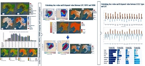
3. Results

This section is presented in three parts: (1) the results of LULC; (2) the results of LST; and (3) an examination as to whether a link exists between these two parameters based on the correlation analysis. In the first section related to LULC, the accuracy assessment for the downscaled land cover maps is presented, and the temporal alteration of the land cover maps is discussed. In the second section, the differences amongst the LST maps are established based on the NDVIs and NDBIs for 2001 and 2018. Finally, the last section analyses the relationship between LULC, LST, NDVI, and NDBI.

3.1. Accuracy Assessment of LULC

The importance of each secondary factor in the LULC classification was identified using RF. The characteristics of these factors were investigated using the GEE platform. The higher the values of the factors, the higher their effectiveness in terms of the classification results. The importance scores related to DEM (elevation) in 2001 (78) and vegetation quality (NDVI) in 2018 (80) were the highest among the factors. The influence of these factors on LULC classification was significant in mountainous and forest areas of Greater Melbourne. The importance of each factor in the classification process is presented in Figure 3.

The accuracy of the land cover maps should be assessed before analysing the spatiotemporal characteristics of the LULC. The accuracy assessment results indicated that the user and producer accuracy indices were approximated to be more than 90% of the downscaled map’s accuracy for all periods.

The results also showed that the overall accuracy was higher than 90% for 2001 and 2018 (90.02% to 90.04%, respectively). The kappa coefficients were 82.1% and 82.3% for 2001 and 2018, respectively. According to previous studies [54,55], if the calculated value of the kappa coefficients is higher than 75, then the classification and reference data are sufficient for accuracy assessment. If the classification accuracy is within the acceptable threshold [51], then the accuracy requirements are met.

Table 6. User’s accuracy, producer’s accuracy, overall accuracy, and kappa coefficient for LULC classification (unit: %).

Land Cover Types	Users’ Accuracy (2001)	Users’ Accuracy (2018)	Producers’ Accuracy (2001)	Producers’ Accuracy (2018)
Forest	89	91	93	88
Shrubs	88	86	89	92
Savannahs	91	91	93	92
Grass	86	91	92	90
Waterbodies	88	89	88	92
Cropland	86	90	90	90
Urban Areas	90	92	91	88
Bare Land	90	92	89	87
Overall Accuracy	90.02		90.04
Kappa Coefficient	82.1		82.03

lists the detailed classification accuracy of each LULC type.

This study utilised Google Earth high-resolution images and the land cover maps from [56] to visually compare them and generated LULC maps of Melbourne in three different locations (for 2001 and 2018). These locations were the CBD area (A), the Werribee Park Golf Club (B), and the Box Hill Train Station (c) (Figure 4). The consistency of the spatial distribution of the main LULC types was considered while conducting the visual comparison between the results of the LULC classification of Melbourne, Google Earth, and Landsat images and the land cover maps from [56].

For instance, in location (A) in the CBD area, besides for urban areas, other types of vegetation that covered those urban areas were more evident in the current study map in comparison to [56]. A similar situation was evident in location (B) near Box Hill Train Station, as these areas are mostly covered with built-up areas; however, the distribution of other land cover types around them was mapped more accurately in the current study.

3.2. Spatiotemporal Characteristics of LULC Changes

The LULC maps of Melbourne and the percentage of each land cover class for 2001 and 2018 are presented in Figure 5 and Figure 6, respectively. Forests, the main LULC type, were found to occupy approximately 32% to 34.5% of the total area of Melbourne. The forests are mainly distributed in the north-eastern areas of the city. The other major LULC classes in Melbourne are urban built-up areas (more than 17%), savannas (15% to 17.5%), grasslands (13% to 13.5%), and croplands (9.5% to 11.5%). Amongst the different land cover types, shrubs and bare lands have the lowest LULC percentage in the study area.

Figure 6 shows the alterations in each LULC from 2001 to 2018. The built-up area percentage increased from 17.81% to 19.4% (from 14,579 to 15,882 hectares) between 2001 and 2018. The bare land percentage increased from 0.65% to 1.35% between 2001 and 2018.

All types of greenery (forests, shrubs, grasslands, and croplands) decreased in their coverage percentages. The percentage of forest areas, crops, shrubs, grasslands, and wetlands also gradually dropped. The decrease in cropland areas (from 92,595 to 78,105 hectares) was the highest amongst the LULC classes. Moreover, the areas of bare lands and savannahs gradually increased. In particular, the savannah areas increased from 15.05% to 17.32% during the study period. Furthermore, the urban built-up areas increased by 1.6% within the same timeline. Notably, the increase in savannah areas (from 126,164 hectares in 2001 to 143,762 hectares in 2018) was more significant than those of the bare lands and urban areas (from 12,319 hectares in 2001 to 14,175 hectares in 2018).

The percentage of urban built-up areas increased notably in Melbourne’s south-eastern and south-western suburbs. One of the significant transformations of land cover types was changing the major LULC classes into urban built-up areas. Furthermore, the vegetation types were replaced by other forms, e.g., grassland to forest (21,437.3 hectares), savannah to forest (41,151.8 hectares), and cropland to forest (18,482.2 hectares) between 2001 and 2018. Notably, a significant are of bare land was transformed into urban areas (1516.99 hectares).

Table 7. The area percentage of LULC types and their alterations in Greater Melbourne in 2001 and 2018.

Urban area 2001 (area percentage)	Urban area 2018 (area percentage)	Urban area alterations from 2001 to 2018 (percentage)
Bare land 2001 (area percentage)	Bare land 2018 (area percentage)	Bare land alterations 2001 to 2018 (percentage)
Grass 2001 (area percentage)	Grass 2018 (area percentage)	Grass alterations 2001 to 2018 (percentage)
Cropland 2001 (area percentage)	Cropland 2018 (area percentage)	Cropland alterations 2001 to 2018 (percentage)

and

Table 8. The area percentage of LULC types and their alterations in Greater Melbourne in 2001 and 2018 (Part 2).

Forest 2001 (area percentage)	Forest 2018 (area percentage)	Forest alterations 2001 to 2018 (percentage)
Savannah 2001 (area percentage)	Savannah 2018 (area percentage)	Savannah alterations 2001 to 2018 (percentage)
Shrubs 2001 (area percentage)	Shrubs 2018 (area percentage)	Shrubs alterations 2001 to 2018 (percentage)
Water 2001 (area percentage)	Water 2018 (area percentage)	Water alterations 2001 to 2018 (percentage)

show the status of the LULC as well as its alterations from 2001 to 2018. The highest values (area percentage) of LULC types in 2001 and 2018 belonged to waterbodies (55.56%, 55.63%) and savannas (57.73%, 60.78%) in Banyule and forests (59.03%, 59.41%) in Bayside.

The most significant increases in the area percentage of the LULC types were for waterbodies in Hume (939%) and bare land (280.86%) in Frankston. In contrast, the main decrease in area percentage of LULC types from 2001 to 2018 belonged to the savannas (−66.67%) in Melton, forests (−59.76%) in Yarra Ranges, and grasslands (−50.40%) in Stonnington.

The most notable increases in urban areas were in Banyule (55.60%), Bayside (31.87%), and Boroondara. In contrast, the decreases in vegetation areas, specifically forest areas, were detected in Stonnington (−31.54%) and Yarra (−29.49%). In addition, among vegetation types, shrubs and cropland faced lower percentages of decreases in comparison to the grass and forest. Shrubs and cropland area percentages increased specifically in Hobsons Bay (66.03%) and Glen Eira (50.64%).

Finally, comparing the LGAs and considering the LULC type alterations from 2001 to 2018 illustrated that some LGAs had fewer alterations in their LULC types. Examples are Maribyrnong in the inner-west area of Greater Melbourne and the City of Melbourne.

3.3. LST Status and Its Relationship with LULC

The statistical parameters of LST for 2001 and 2018 indicates that. both minimum and maximum values of LST in 2018 were higher than those in 2001. The minimum LST in Melbourne in 2018 was recorded as 15.25 °C, which is 3.7 °C higher than the minimum LST in Melbourne in 2001 (11.55 °C). The maximum LST in 2018 was recorded at 46.4 °C, which is 1 °C higher than the maximum LST in 2001 (45.4 °C). The difference indicates that Melbourne’s average LST increased over the selected study period. The LST frequency for Melbourne in 2001 was the highest, at 27.5 °C, which was 5.5 °C lower than in 2018 (33 °C).

In 2001, the LST in Melbourne ranged from 26 °C to 28 °C. Figure 7 shows that most parts of Melbourne, except the western, north-eastern and south-eastern suburbs, had LSTs within this range. In 2018, the temperature range increased from 31 °C to 33 °C, signifying a 5 °C increase in LST from 2001 to 2018 in most parts of Melbourne.

The western suburbs showed different ranges of temperature in 2001 (between 14 °C and 16 °C), increasing to the range of 20 °C–23 °C in 2018. This scenario signified a 6.5 °C increase in the average LST in these areas from 2001 to 2018. The highest LSTs recorded in summer (>30 °C) were captured within the high-temperature variation zones. These zones are primarily located in the city’s south-eastern suburbs, occupying 12% of Melbourne’s total area.

Figure 8 shows the mean values of LST for each LULC class. The highest LST values (46.03 °C) in 2001 were recorded for the urban-built-up areas, particularly in the Melbourne CBD. High levels of impervious surfaces, lack of green coverage, and high levels of anthropogenic heat caused by humans and transportation could explain the highest LST being recorded in this area. By contrast, the lowest values of LST were recorded for the forest areas at 11.5 °C. In 2018, croplands (46.42 °C) and savannahs (46.33 °C) had the highest maximum values, whereas the minimum values of LST were recorded for the shrub and forest LULC classes at 15.25 °C and 16.39 °C, respectively.

The findings indicated that the LST for all LULC types increased between 2001 and 2018. The mean LST for bare lands was 24.02 °C in 2001, increasing to 29.67 °C in 2018 (a difference of 5.65 °C). Similarly, the urban areas recorded a mean LST of 26.91 °C in 2001, increasing substantially to 32.86 °C in 2018 (a difference of 5.95 °C). The maximum change in the mean LST values was recorded for the shrub and grass LULC classes at 12.18 °C and 10.66 °C, respectively. The significant change recorded for these LULC classes can be linked to the rapid urban expansion that occurred between 2001 to 2018, suggesting a significant drop in the percentage of these LULC types, consequently affecting the average LST.

3.4. NDVI Status and Its Relationship with LST

The negative skewness of NDVI was −0.54 in 2001, and it decreased to −1.1 in 2018. The decline indicated that the NDVI values were left-skewed. Furthermore, the NDVI kurtosis values were recorded to be 4.1 in 2001 and 5.2 in 2018 (higher than 3), indicating that their distribution was normal. In addition, the low STD values of NDVI were 0.1 in 2001 and 0.09 in 2018, meaning the NDVI values were closer to their mean values.

Figure 9 shows that 72% of Melbourne was covered with NDVI, ranging from 0.25 to 0.50 in 2001, covering most of Melbourne, but the inner CBD and the western and eastern parts of Melbourne were excluded. By contrast, the lowest NDVI range values were below 0.02 and were mainly recorded in the Melbourne CBD, inner-south-eastern, and inner-south-western suburbs, particularly the areas close to the ocean. For 2018, the NDVI range did not change, as the values had the same range (0.2 to 0.5) for most parts of Melbourne (81% of the Melbourne area). The areas falling under the NDVI range of 0.25 to 0.5 increased from 72% to 81% in 2001, signifying an increase in the area covered by sparsely vegetated LULC classes (including shrubs and grasslands). The NDVI range from 0.2 to 0.5 mainly covered the eastern parts of Melbourne. Low values of NDVI (below 0.02) were observed primarily in the inner-western areas.

Figure 10 shows the low negative correlation and linear relationship between LST (summer daytime) and annual mean NDVI values for both 2001 (r: −0.386, R²: 0.148) and 2018 (r: −0.435, R²: 0.189). The r-value between NDVI and LST in 2018 was lower than in 2001. However, based on the analysis, higher values of the coefficient of determination (R²) were manifested in 2018 (0.189) compared with 2001 (0.148). The STD values of NDVI were calculated to be 0.182 in 2001 and 0.184 in 2018. This indicates that the NDVI values were clustered around their mean values, particularly 0.32 in 2001 and 0.34 in 2018.

Figure 11 shows the spatial distribution of r-value between NDVI and LST in 2001 and 2018. A positive r-value existed between NDVI and LST, particularly in the northern, south-eastern, and coastal areas for 2001 and 2018. Comparing NDVI and LST maps in 2001 and 2018 showed that most parts of Melbourne had a positive r-value. In 2001, 67.80% of Melbourne was covered with a positive range of r-values from 0.01 to 1. In 2018, 92.84% of Melbourne was covered with a positive r-value range from 0.06 to 1. The inner-city and north-eastern and north-western parts of Melbourne signified an inverse relationship between NDVI and LST. In 2001, this inverse relationship (negative r-value) varied from −1 to 0 and covered 32% of Melbourne’s areas. By contrast, in 2018, the same range of negative r-values (−1 to 0) covered 7.15% of Melbourne.

The results aligned with the findings of several studies [57,58] showing that the relationship between NDVI and LST is largely affected by surface types and land cover. The results of this study were also aligned with the findings of [57,59], in which the authors found a positive correlation between LST and NDVI, especially in waterbodies and salt ponds. One of the major changes depicted between 2001 to 2018 was the transition of the inner-south-eastern, western, and inner-northern areas from the negative r-value range (−0.08 to 0.2) to the positive r-value range (0.28 to 0.44).

Figure 12 shows the R² values between NDVI and LST. The R² values were closer to 1 for most parts of Melbourne from 2001 to 2018. However, this pattern was only seen in the eastern and north-eastern parts in 2001.

3.5. NDBI Status and Its Relationship and LST

The statistical analysis of NDBI in 2001 and 2018 showed that both maximum and minimum values of NDBI in 2001 (0.45, −0.77) were higher than those in 2018 (0.34, −0.54). However, the frequency of positive NDBI values was higher in 2018, which indicated an increase in the built-up areas from 2001 to 2018.

Figure 13 shows the spatial distribution of NDBI in Melbourne in 2001 and 2018. More than half (53%) of Melbourne’s areas were covered by the NDBI range of −0.19 to −0.06 in 2001. This range covered most parts of Melbourne, except the forest areas in the north-eastern suburbs. In 2018, 61% of Melbourne areas were covered by the NDBI range of −0.28 to −0.8. This range was primarily captured in the south-eastern suburbs. The spatial distribution of NDBI also showed that the areas with NDBI values more than 0 (built-up areas) mainly expanded towards the south-eastern and north-western suburbs.

In addition, the statistical analysis of the NDBI for each class of land cover in 2001 and 2018 showed that the maximum NDBI value for urban areas increased from 0.28 in 2001 to 0.34 in 2018 (+0.06), and the maximum NDBI value for vegetation cover decreased from 0.34 to 0.27 (−0.07).

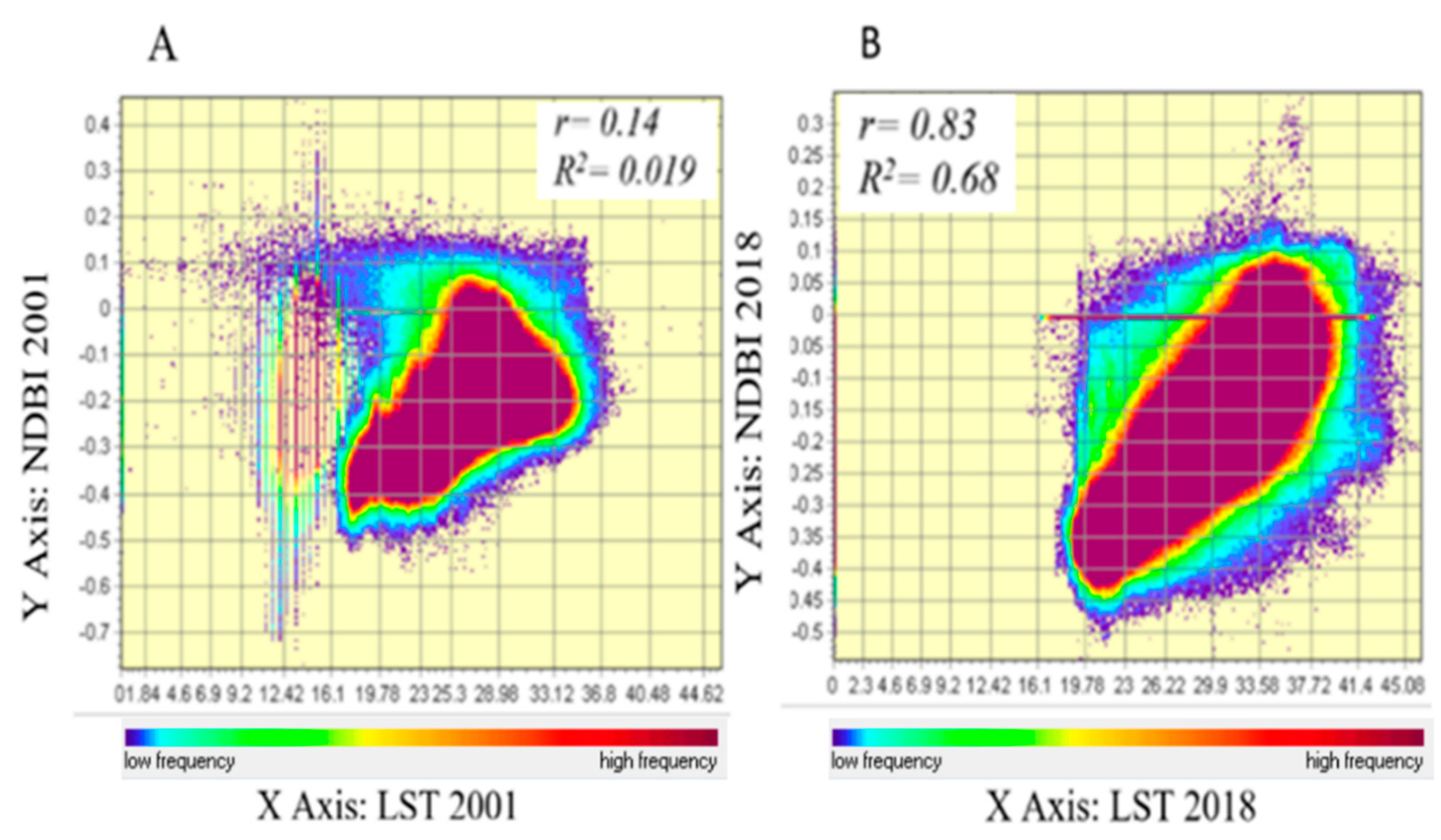
According to Figure 14, a positive correlation and linear relationship existed between LST and annual mean NDBI values in 2001 (A) (r: 0.14, R²: 0.019) and 2018 (B) (r: 0.83, R²: 0.68). The NDBI and LST had higher r-values during the summer of 2018, and their R-squared values explained at least 70% of the variation of the LST, as explained by the NDBI. This was also the case for NDVI; the lower STD values of 0.10 in 2001 indicated that the database was more clustered around the mean temperature than that in 2018. In addition, the alteration of LST based on the NDBI was faster in 2018 than in 2001.

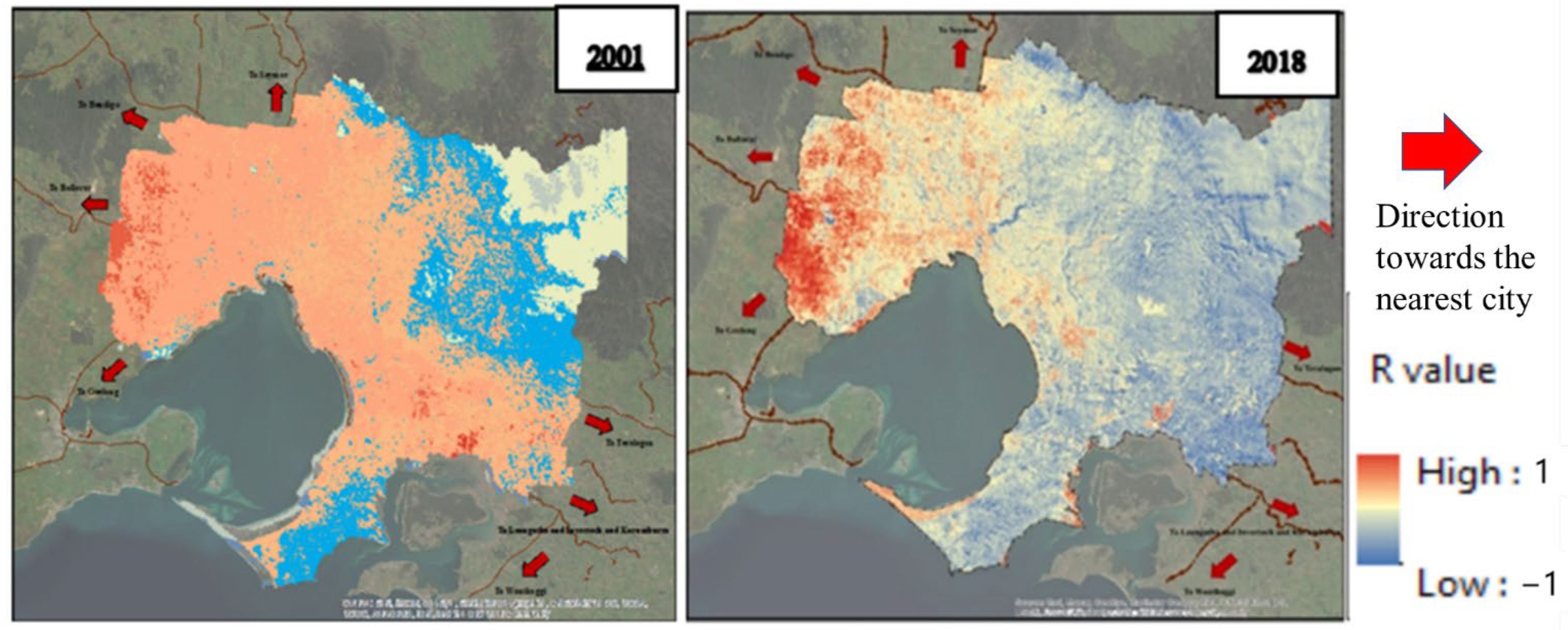
Figure 15 shows the spatial distribution of r value between NDBI and LST in 2001 and 2018. A positive r-value existed between NDBI and LST, particularly in the inner-metro areas and south-eastern and western suburbs of Melbourne, in 2001 and 2018. Comparing NDBI and LST maps in 2001 and 2008 shows more areas covered with a positive r-value for 2018 (21% of Melbourne’s area).

3.6. LULC and LST Association Considering NDBI and NDVI

This section first investigated the max, min, and mean of each LULC type in 2001 and 2018. Furthermore, based on the zonal statistical analysis, the r-value and coefficient of determination (R²) between each LULC type and LST were identified based on the NDBI, NDVI, and LST relationship.

Figure 16 shows that savannahs (0.84), grass (0.78), and forests (0.74) had the highest maximum NDVI values in 2001. By contrast, in 2018, the highest maximum value of NDVI was for forests (0.40). Concerning vegetation quality, high values of NDVI are related to high quality vegetation [60]. The mean values of NDVI in 2001 showed that grasslands (0.41) had the maximum level of health among the vegetation types in the study area. In 2018, the vegetation quality was at the maximum for forest (0.30) and savannah (0.28) areas, showing higher mean NDVI values than the other LULC classes. According to Figure 16, the mean NDVI value for urban areas increased from 0.19 in 2001 to 0.25 in 2018 (+0.06), and the mean NDVI value for vegetation covers decreased from 0.35 to 0.30 (−0.05) for forest areas, and from 0.30 to 0.28 (−0.02) for savannas during 2001 to 2018.

Figure 16 also shows that the absolute mean NDBI value for urban areas increased from 0.10 in 2001 to 0.25 in 2018 (+0.15), and the mean NDBI value for forest and grass areas decreased (−0.6).

Figure 17 indicates that in 2001, the forest had the highest R² values (0.88) with LST considering its NDVI value index. Following the waterbodies, shrubs and cropland had the highest R² values with LST in 2001. Furthermore, the forests and waterbodies in 2001 contributed more to altering the LST and cooling down the temperature than other vegetation types. In 2018, among land cover types, grass (0.48), forests (0.27), shrubs (0.21), and savannas (0.17) had important contribution to the LST decrement. It is clear from Figure 17 that the R² value for all the land cover types decreased from 2001 to 2018, and the most drastic change was related to the urban areas and bare lands.

In 2001, most land cover types had a lower R² value considering the NDBI. The highest R² values belonged to the grass (0.38), bare land (0.34), and urban areas (0.3). In 2018, R² values increased: urban areas (0.64), bare land (0.62), cropland (0.61), and grass (0.46). These land cover types contributed the most to LST increments from 2001 to 2018.

4. Discussion

4.1. Importance of Various Factors in LULC Classification

The analysis of the importance of each variable on LULC classification between 2001 and 2018 shows that elevation has a significant contribution to LULC classification due to the high elevation of the Greater Melbourne area, especially around the north-east. The elevation significantly impacts the spatial distribution of precipitation, temperature, and vegetation types.

For instance, various locations in Melbourne show different trends in elevation and temperature association. Mathew, et al. [61] listed some factors that affect the association between elevation and temperature for specific days, nights, and seasons. Some of these factors are solar radiation, angle of incidence of solar radiation, surface roughness, types of land cover, moisture content, weather conditions, and the extent of vegetation.

The spatial distribution of various land covers, such as farmland and waterbodies, is also affected by the elevation [62]. Accordingly, the spatial distribution of other factors, such as NDWI and NDVI, is affected by the elevation and, in fact, results in a variation of the spatial distribution of waterbodies, grasslands, farmlands, and forest areas [63].

From 2001 to 2018, according to the users’ accuracy and producers’ accuracy of LULC classification results, the classification accuracies of urban lands, bare lands (user’s accuracy), and savannahs and grassland (producer’s accuracy) were the highest. The higher accuracy values are potentially due to concentrated areas of bare lands, urban areas, grassland, and savannahs in Greater Melbourne, specifically in the eastern and inner areas. Notably, sometimes some farmland, cropland, and even urban areas are not classified properly, which may be due to the amalgamation of the grassland with them, resulting in similar spectral characteristics between farmland and urban areas, and between cropland and grassland.

4.2. Spatio-Temporal Variation of the LULC and Their Roles in LST Condition

In this study, forests and savannahs were the main LULC type in Greater Melbourne, followed by urban land, which is mainly consistent with the global LULC products [64]. Our LULC classification results indicated that the percentage of built-up areas increased dramatically. Furthermore, the total bare land area increased by 53% between 2001 and 2018. The substantial increase in bare lands from 2001 to 2018 can be explained by the large level of transformation of vegetative areas into bare lands. Furthermore, the vegetation coverage was reduced from 2001 to 2018 and mainly converted to built-up areas. The savannah areas expanded from 2001 to 2018, and the difference can probably be attributed to the continuous implementation of urban forest projects in Greater Melbourne [65]. In contrast, the expansion of construction projects and accelerated development that was dominant in inner areas of Greater Melbourne led to more urban lands in 2018. Most of the bare land has been converted into built-up areas in most parts of Melbourne.

The intensity of the land-use change is more apparent in the south-western areas of Greater Melbourne, where there are transitions from grasslands and bare lands to urban areas. These areas mainly have relatively flat terrain suitable for construction projects, and the land exploitation is relatively high. However, the eastern part of Greater Melbourne is high in elevation, and people have already settled in those areas, so the degree of land use development is low. In fact, the high elevation and higher amount of vegetation limit this area’s urbanisation process and generate a limited opportunity for land expansion. The alterations of the environmental conditions (mainly the NDVI and elevation in this study) could potentially change the process of LULC variation. Our results showed that the synergy between the LST and LULC changes was different. From 2001 to 2018, the LST values gradually increased due to the LULC changes, especially in the grassland areas, similar to the findings of [66,67]. Furthermore, the increase in LST mainly dominated the south-eastern, inner-metro, and north-western suburbs, occupying 15% of Melbourne’s area. Proximity to industrial zones (e.g., north-western suburbs), high levels of anthropogenic heat, and lack of vegetative coverage (e.g., inner-metro regions) and the sudden increase in the magnitude of built-up areas (e.g., south-eastern suburbs) could explain the increase in LST in these areas over the selected timeframe.

Several cities, such as Shenyang and Kuala Lumpur metropolitan area [68,69], show patterns similar to Greater Melbourne, with urban land recording the highest temperatures among the land-use classes and, in contrast, the lowest being recorded for the waterbodies and forest areas. In fact, the specific heat capacity of water and urban trees is higher than that of soil and impervious surfaces, which results in a higher temperature. Notably, Greater Melbourne is a coastal city with several rivers and many forest areas. In addition, comparing the lowest temperature of waterbodies and forest areas in Greater Melbourne and other studies such as KJ, et al. [70] could potentially be related to the percentage of each land cover type (waterbodies, forest, etc.) in various cities.

The variation in daytime LST values of urban land area and forest was significant between 2001 and 2018 in the summertime but more considerable by 2018. This is consistent with the results of other studies in Barcelona and Rotterdam [71,72]. The main reason for the LST difference is related to the ability of various surfaces to receive solar radiation. Furthermore, urban development from 2001 to 2018 increased the number of areas with low tree cover and high impervious surface densities in the inner parts of Greater Melbourne. Other studies conducted in different cities around the world [73,74] acknowledged that the LST of green areas (mainly forests) is lower than the impervious surfaces (urban lands).

4.3. LST, NDVI, and NDBI Association

The relationship between NDVI and LST has been widely studied in different cities around the world, such as in Shanghai, China [75]; Mashhad, Iran [76]; and Melbourne, Australia [16]. The results from those studies showed a negative correlation between NDVI and LST. However, the amount of R-value and R-squared values differed for each city depending on the geospatial characteristics, LULC types, climatic factors and evapotranspiration rates of plants [77].

The inverse direction concerning the association between LST and NDVI has been mentioned in many studies conducted in different cities worldwide [57,58]. Their association is affected by various surface types and land cover types. Moreover, the NDVI trend also depends on elevation and land cover types. The positive association between LST and NDVI, especially in waterbodies and salt ponds, is also mentioned in studies conducted by Deng, et al. [57] and Chi, et al. [59]. The variety of association values between LST and NDVI in some east-side areas of Greater Melbourne is related to the types of land use and land cover types in these areas. For instance, green areas could lead to cooling temperatures, whereas built-up and bare lands are the main reasons for the temperature increase [78].

The complex association between NDVI and LST could exist for various reasons. For instance, Sandholt, et al. [79] and Lambin and Ehrlich [80] mention the critical role of surface moisture in LST and NDVI association. In the current paper, a negative association between LST and NDVI was shown to increase when the soil moisture content increased. This situation is consistent with the findings of Guha and Govil [78]. Furthermore, the current research found that the inverse association between LST and NDVI is more evident in the north-east and inner-north-east LGAs covered with dense vegetation, which aligns with the results of Chi, et al. [59]. One of the main reasons behind this inverse association is the leaves of trees and plants that prevent rainfall from being absorbed by the soil. Furthermore, vegetation in these areas absorbs a large amount of the soil’s water. Thus, the soil’s moisture content will reduce. In many cases, LSTs have an inverse association with soil moisture content. The LSTs in areas with high moisture content increase gradually due to the evaporation absorbed by heat [81].

The positive association between LST and NDBI detected in the current research is consistent with most prior studies [82,83,84]. This association demonstrates that built-up areas, plus bare and fallow land, are responsible for high values of LST. Some studies, such as Feng, et al. [85] and Guha, et al. [83], show that the NDBI and LST association is affected by the land cover types and seasonal changes, similar to the NDVI and LST association. Similar to NDVI, various r and R² values were detected in different cities and are governed by different physical, environmental, and climatic factors [86]. For instance, in Melbourne, the negative range of the NDBI is most likely associated with forest land cover, waterbodies, and agricultural land. In contrast, higher NDBI values are related to built-up urban areas.

One of the main reasons for the inverse association between NDBI and LST is related to the city’s expansion, which caused LST value reduction [87]. Furthermore, a study by Mpakairi and Muvengwi [88] showed that NDBI, in some cases, is a minor contributor to predicting LST because the aerial extent of built-up areas remains the same for urban and suburban areas. Notably, NDBI has a high spectral confusion rate between bare and urban areas. Another reason is that built-up surfaces reflect less incoming solar radiation than expected. In the case of Melbourne, the inner-city and the western and south-western suburbs showed a negligible positive relationship between NDBI and LST. This finding aligns with the results of previous studies [84].

4.4. Land Cover Types’ Contributions to LST Alteration

According to the relationship between NDBI and LST, the positive contribution of urban and built-up areas to increasing the LST is identified as one of the important factors in 2018 (R² = 0.64) compared to 2001 (R² = 0.30). This situation indicated the key contribution of urban expansion to the LST increment in Melbourne, similar to Harmay, et al. [20]. In contrast, according to the relationship of the LST and NDVI, the forest (R² = 0.27), grass (R² = 0.48) and shrubs (R² = 0.21) had mitigation impacts on LST in 2018 in comparison to other types of land cover. The mitigation impact of the urban vegetation in this study was consistent with Liu, et al. [89] and Ke, et al. [90]. In 2001, vegetation types had more significant impacts on LST, especially forests (R² = 0.88) and shrubs (R² = 0.78). The cooling effect of these types of vegetation, such as grass, is mentioned in Salleh, et al. [91] and Shen, et al. [92]. These studies indicated that the vegetation types have a lower surface albedo and high surface heat capacity. Indeed, the variations in evapotranspiration and albedo affect the latent heat flux (evaporative cooling) and net shortwave radiation.

It is expected that the higher R² value for the forest LULC type is due to the combined effect of shading and evapotranspiration; however, the evaporative cooling differs based on the type of tree species according to their various physiological traits [93]. The variety in physiological characteristics could result in different R² values for forest and savannah classes in Greater Melbourne. Simultaneously, microclimatic factors such as humidity, wind flow, soil moisture, and precipitation rate impact these vegetation types’ cooling effects in different Melbourne locations [94,95].

Sometimes, in both 2001 and 2018, the cooling effects of the LULC types related to the vegetation are close to each other in terms of their R² values. Examples are forest and shrub land types. Indeed, the capacity of these LULC types to reduce LST is not equal in all parts of Melbourne. The reason may be related to the composition and configuration of vegetation types in Melbourne, the structural and biophysical characteristics of vegetation, or the microclimate conditions of various locations in the city [96,97,98].

Similar to Zhao, et al. [99] in Beijing, these types of LULC were potentially planted together and led to a potential synergic cooling effect. The significant cooling effect of the grass in 2018 is similar to the findings of Shashua-Bar, et al. [100]. The results of the mentioned study showed that grass can provide greater cooling when it is shaded.

Like the vegetative types of the LULC, planting grass with impervious surfaces could be a potential reason for having a high R² value for this type of LULC. Indeed, in 2001, the composition of the urban areas had a limited impact on LST, while grass, in this case, altered the LST more intensely. In 2018, in addition to having more urban areas, other details such as the colour of the rooftops and building sizes, heights, geometry, and materials played a role in increasing the LST value.

4.5. Potential Impacts of Climate-Related Changes in Melbourne

The evaporative cooling variation affects the drought conditions and water restrictions in Melbourne, which also impact the temperature difference between urban and rural areas [101]. During this period, the water retention in the vegetation areas was higher than in urban areas, which can be seen in the results section. Indeed, the area percentage of water in 2001 was higher in the Cardinia and Mornington Peninsula rural areas. This status is also related to the soil moisture and vegetation fraction.

Higher rainfall values and cloud cover fractions during 2010 and 2011 were the major factors in the high efficiency of the convective heat transfer in Greater Melbourne. However, note that the convective heat transfer was less efficient in dissipating the heat from urban areas in comparison to rural areas [102], as the alterations of urban areas are more intense in Greater Melbourne’s rural areas. Furthermore, the intensity of urban area alterations was highlighted as a more important factor than vegetation density, considering its impact on convection [102]. Finally, the high temperature and its fluctuation from 2011 to 2018 were mainly due to the high heat storage release of impervious surfaces during the day [103] and the change in direction and wind speed intensity.

4.6. Advantages and Limitations of the Current Study

The GEE cloud computing platform can process massive amounts of geographic data [104]. Furthermore, the image cloud removal and training sample can quickly and accurately be applied to the Melbourne LULC classification based on GEE. Although GEE has numerous advantages, there are some computational limitations, such as calculation timeout, the exceeding of user memory, and limitations of the output size [105].

Notably, the effect of anthropogenic factors, transportation, and the contribution of socio-economic factors on LULC classification in Greater Melbourne could be considered in addition to the ancillary factors (the mainly environmental factors mentioned in this study) so as to establish a comprehensive model that integrates multi-source data.

5. Conclusions

This study analysed the impact of the change in LULC on LST over 17 years (2001–2018) in Melbourne using remote sensing satellite imageries. The spatiotemporal pattern of the LULC changes was measured for the selected years, and eight different LULC classes, including forest, shrub, savannah, grass, waterbodies, cropland, urban areas, and bare land, were identified. In addressing the study objectives, the spatiotemporal patterns of LST, NDVI, and NDBI; the fluctuations in LST with respect to LULC classes; and the variations of LST in relation to NDVI and NDBI were studied.

The findings revealed that the percentage of built-up areas increased dramatically from 1434 to 1588 km² between 2001 and 2018. The total bare land area increased by 53% between 2001 and 2018. The substantial increase in bare lands from 2001 to 2018 can be explained by the significant level of transformation of vegetative areas into bare lands. Furthermore, the vegetation coverage was reduced from 6413 km² in 2001 to 6263 km² in 2018 and mainly converted to built-up areas. Therefore, most parts of the bare land have been converted into built-up areas in most parts of Melbourne.

According to the LST analysis, the south-eastern and north inner-eastern parts were the hottest locations in Melbourne in 2001. However, the hottest places found in 2018 were located in the north-western, inner-city, and south-eastern areas. The lowest LSTs were detected in the north-eastern forest areas in both 2001 and 2018. High humidity and evapotranspiration rates for the areas closer to the ocean, lower levels of soil moisture in north-inner-eastern parts of Melbourne, and high levels of impervious surfaces in the inner-city (CBD) were the leading causes of the variations in LST between 2001 and 2018.

The mean LST in 2001 was 25.4 °C, which increased to 30.5 °C. The mean LST for vegetation coverage increased from 25.3 °C to 30.8 °C. The mean LST in 2001 for built-up areas increased from 26.91 °C to 32.86 °C between 2001 and 2018. This increase in bare land was from 24.2 °C to 29.67 °C. Therefore, the maximum increase in LST occurred in built-up areas from 2001 to 2018.

The findings of this study also demonstrated an indirect correlation between LST and NDVI, whereas a direct correlation was found between mean LST and NDBI for both 2001 and 2018. Different LULC classes have a substantial impact on temperature. In 2001, the forest had the highest R² values (0.88) with LST. In 2018, grass (0.48) had the most important contribution to LST reduction in land cover types. The R² value for all the land cover types was reduced from 2001 to 2018, and the most drastic change was related to the urban areas and bare lands. In 2001, most land cover types had a lower R² value considering the NDBI. The highest R² value belonged to grass (0.38). In 2018, R² values increased, and the highest value belonged to the urban areas (0.64).

This study’s results highlight the need to determine effective heat mitigation strategies and accordingly reduce the adverse impacts on urban climate of the increase in impervious surfaces in urban areas. Given the limited available lands in cities, one of the most promising measures to mitigate urban overheating is integrating and promoting green areas in urban areas in different forms.

The findings of this study can benefit urban planners and various stakeholders in making strategic decisions for future urban growth without compromising the environment and, in particular, minimising the threats brought on by ongoing climate change. Furthermore, as Melbourne’s population reaches 8 million in the near future (2050), future studies could predict the land use and land cover change and LST or use the high-resolution imageries of LST and land cover maps and investigate their relationship.