A Multistage Time-Delay Control Model for COVID-19 Transmission

Abstract

With the transmission of the COVID-19 epidemic at home and abroad, this paper considers the spread process in China, improves the classic epidemic SEIR model, and establishes a multistage time-delay control model (MTCM) for COVID-19 transmission. The MTCM divides the spread of COVID-19 into three periods: the outbreak period, the control period and the steady period. The classical SEIR model, the improved SEQIR model and the SEQIR Ⅱ model correspond to the three periods. The classical SEIR model was adopted for the outbreak period and yielded results that were consistent with the observed early propagation of COVID-19 transmission. In the control period, adding isolation measures and a time delay to the MTCM and adjusting the rates yielded a better simulation effect. In the steady period, the focus of consideration is the number of new patients, population movement (in-migration and out-migration of the population) and patient classification (symptomatic and asymptomatic patients). The MCTM was used for simulation, and the comparison results revealed that the simulated data of the MCTM (improved SEQIR model) and the actual data are similar in the control period. The control policy of isolation measures is effective. New infections, population flow and patients with symptomatic or asymptomatic symptoms are more consistent with the steady period characteristics. The multi-stage time-delay control model for COVID-19 transmission provides theoretical methods and good prevention and control measures for future epidemic policy formulation.

1. Introduction

The coronavirus disease 2019 (Corona Virus Disease 2019, COVID-19) pandemic across the globe is still a serious “public health event of international concern” and “major crisis” and is expected to remain so for some time to come. As of February 2021, 222 countries and regions have been affected. More than 100 million confirmed cases have been reported worldwide, and more than 100 countries have reported at least 10,000 patients [1]. The virus that causes COVID-19 spreads rapidly and has a wide range; it causes serious harm to human health, is a national biosafety concern, and has a huge impact on social stability and economic development. Many countries have a national epidemic strategy response to COVID-19, and the national strategic response to the COVID-19 epidemic situation data were collected [2]. At present, the COVID-19 epidemic in China has been basically controlled, but small-scale outbreaks continue to occur from time to time. Moreover, the global epidemic is still spreading. How to control infectious diseases has become a topic of concern to all countries in the world. Therefore, the focus of this paper is to study the transmission rules of COVID-19 in three stages and verify the effectiveness of prevention and control measures.

In this paper, with the development of the COVID-19 epidemic at home and abroad, many factors are related to the spread of this disease in China, including medical conditions, national policies, testing equipment, isolation measures, etc. A multistage time-delay control model (MTCM) is used to simulate the spread of COVID-19. The classic SEIR (susceptible–exposed–infected–recovered) epidemic model is improved. In the MTCM, COVID-19 transmission can be divided into three periods: the outbreak period (no measure intervention), the control period (adopt effective isolation measures, add time delay and improve multiple rates), and the steady period (include migration factors, and distinguish between symptomatic and asymptomatic patients). Because of the incubation period, the government adopts prevention and control measures to isolate groups that have been in close contact with confirmed patients.

The time delay factor is added to the MTCM, which typically occurs in isolating the close contacts of confirmed patients, recovering the patients and improving the medical measures, and that changes the rates. In this paper, including three phases in the MTCM, different parameters and rates are used to simulate different phases. Based on the World Health Organization (WHO)’s official data for China, through referring to the literature, the actual data and simulation results of the MTCM analysis, the effectiveness of the prevention and control measures is verified, and the simulation effect is good. A multistage time-delay control model for COVID-19 transmission was obtained.

The specific contributions of this paper include:

(1)

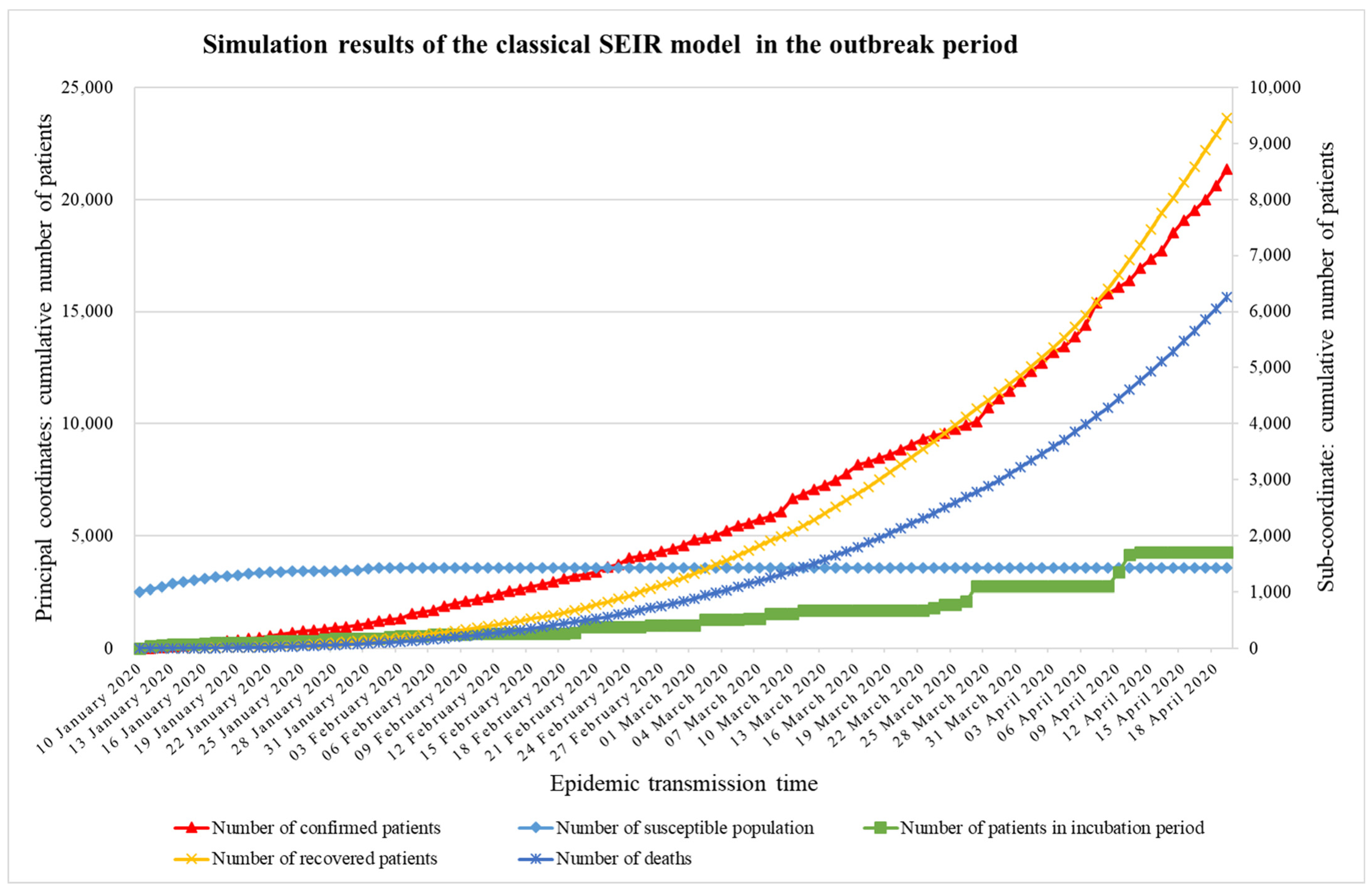
Based on a survey of the literature on epidemiology, due to the three periods of the development of the epidemic, a multistage time-delay COVID-19 transmission model is established in this paper. The classic SEIR model, the improved SEQIR (susceptible–exposed–quarantine–infected–recovered) model and the SEQIR Ⅱ (susceptible–exposed–quarantine–infected–recovered Ⅱ) model are adopted and used to model the outbreak period, the control period, and the steady period, respectively. These models could better simulate the transmission of three phases of COVID-19, and the results are more actual with the development of the epidemic.

(2)

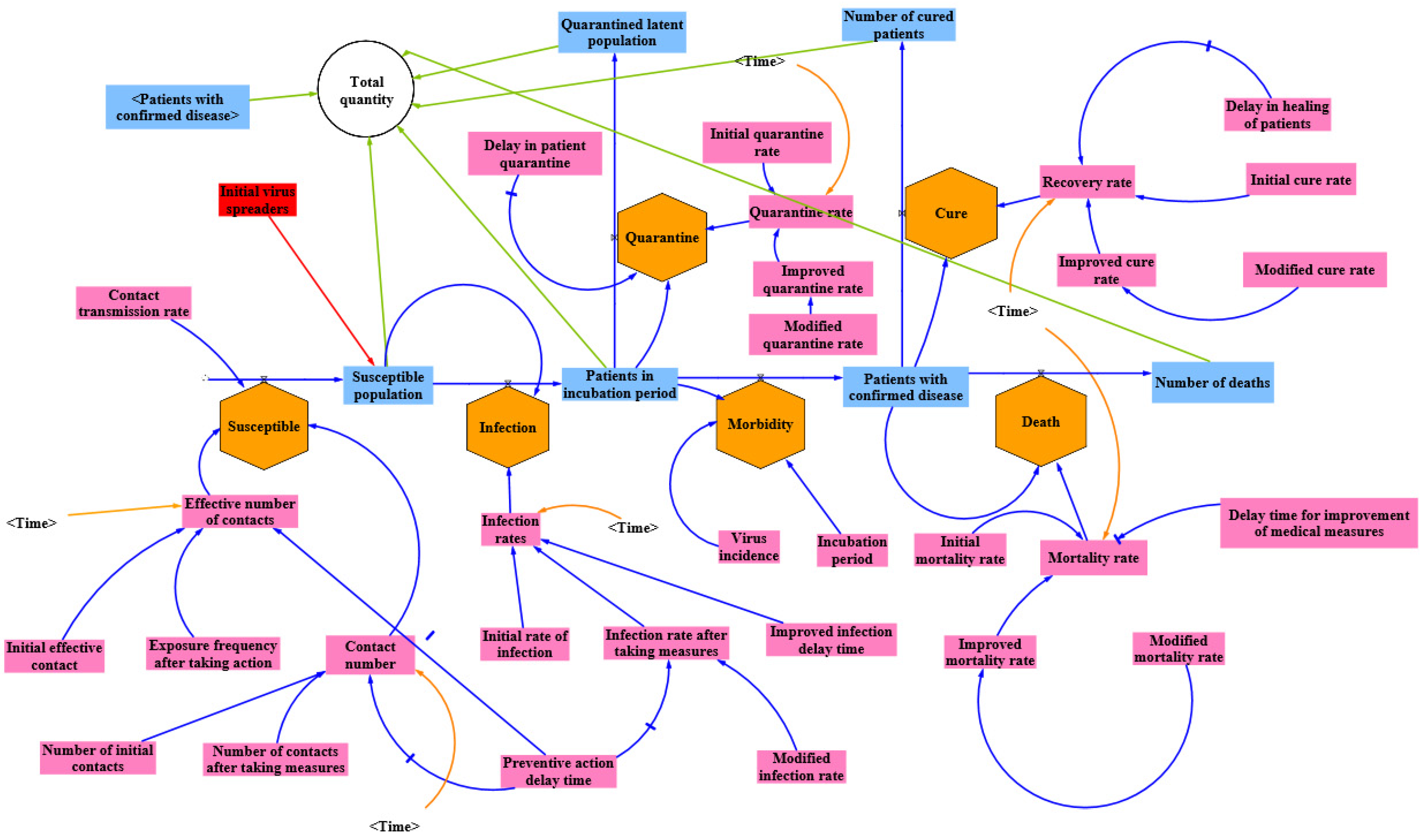
Because COVID-19 has an incubation period, the state shall adopt prevention and control measures designed to provide prevention and control, isolating the close contacts of confirmed patients until they are cured; isolation, the spread of death and medical measures such as process improvement have a time lag. In this paper, the SEQIR model adds the isolation measures Q, considering the effective time of Q, that is, the delay time as a delay factor. In addition, several change rates are improved to better simulate the results.

(3)

Population mobility has a significant impact on the spread of COVID-19. The SEQIR II model used in this paper takes population mobility during the steady period, which includes both immigrating and emigrating populations.

(4)

In the steady period, this paper’s focus shifts from the cumulative number of confirmed patients to the number of new patients. In addition, the symptoms of patients are classified as asymptomatic and symptomatic. Therefore, at the beginning of the steady period, the new patients could be divided into symptomatic patients and asymptomatic patients, a division that is more consistent with the current transmission situation.

The rest of this paper is organized as follows: Section 2 discusses related work, followed by the model hypothesis and parameter design in Section 3. The SEIR and SEQIR II models are discussed in Section 4. Section 5 presents the simulation results and compares them with actual data, and Section 6 concludes the paper with a summary and future research directions.

2. Related Work

In the process of fighting COVID-19, domestic and foreign scholars have conducted a great deal of research on the prediction, prevention and control of the spread of new coronary pneumonia. Spann W et al. [3] analyzed the structure and gene expression of the new coronavirus. Zhu et al. [4] explained that COVID-19 is a novel coronavirus and its diagnostic method. Chen et al. [5] introduced its genome structure, replication, and pathogenesis. They have both explained and illuminated the cause of the outbreak of COVID-19 from a medical perspective. For the study of infectious diseases, many scholars have adopted different research methods, such as genetic algorithms [6], particle swarm optimization algorithms [7], logistic algorithms [8] and others.

The results of this research have played a positive role in the judgment, decision-making, and treatment of the epidemic. The main models used in this research are the SIR (susceptible–infected–recovered) model, the SEIR model and other related models. The SIR model only considers the susceptible, the infected and the evacuated, while the SEIR model also includes exposed individuals; other related models include the stochastic dynamic model, the dynamic model of emerging infectious diseases and others.

Regarding the SIR model, Mei et al. [9] combined that model with the extreme learning machine literature in machine learning based on the SIR model. Law et al. [10] modified the SIR model to specifically simulate the early depleting transmission dynamics of COVID-19 to better predict its temporal trend in Malaysia. Projections generated based on observed data are useful for future planning and control of COVID-19. Santos et al. [11] used an adaptive susceptible–infected–removed (SIR) model with dynamic recovery and transmission rates. This model reproduces the number of confirmed cases over time with an error of less than 5%, and short-term and long-term predictions are provided. The model can also be used to account with great accuracy for the dynamics of the epidemic in other countries.

Regarding the SEIR model, Guerrero-Nancuante et al. [12] analyzed the new coronary pneumonia in China through the generalized SEIR model for Hubei, Wuhan, Beijing and Shanghai and used sensitivity analysis to derive the main prevention and control measures. Wu et al. [13] used the SEIR model to predict the scale of the epidemic in Wuhan at that time and the peak of the epidemic in Wuhan and the rest of the country. Yang et al. [14] improved the SEIR model by considering population mobility and used the improved model to predict the domestic epidemic trend. Walker et al. [15] used the age-based SEIR model to predict the number of infections and deaths in the United States.

Regarding the epidemic model, Driessche et al. [16] used an SIS epidemic model with a non-constant contact rate that may have multiple stable equilibria, a backward bifurcation and hysteresis. The analysis includes both local and global stability of equilibria. YongliCai et al. [17] investigated the global dynamics of a general SIRS epidemic model with a ratio-dependent incidence rate and provided analytic results regarding stochastic boundedness and permanence/extinction. Chen et al. [18] proposed a time-dependent SIR method that is better than the traditional static SIR model as it can adapt to the change in contagious disease control policies such as city lockdowns.

Many scholars have applied other related models to study the spread of the epidemic. Guo et al. [19] proposed a limit IR model that transformed the construction of the forecasting model of the epidemic development trend into the construction of a forecasting model for model parameters, and predicted the national epidemic trend. Boldog et al. [20] used simulation calculations to assess the risk of a new coronavirus outbreak outside China. Du et al. [21] used the coupling method of the exponential growth model and the random movement model to estimate the risk of the new coronavirus emerging in 369 cities in China prior to the closure of Wuhan.

Since COVID-19 has an incubation period and confirmed patients may recover, there is a time lag in the improvement of medical measures for the control and treatment of the disease, and the classic infectious disease model reflects neither this time lag relationship nor the impact of policies and medical resources on the epidemic in China. Therefore, only by integrating intervention measures [22,23], medical conditions and time lag relationships into the classic epidemic model can we accurately predict the epidemic trend [24], peak time and end time of COVID-19 in China. Based on the existing research [25], this article comprehensively considers the impact of multiple factors such as medical conditions, national policies, testing equipment, isolation measures, and virus transmission characteristics. Combined with the development process of the epidemic in China, the SEIR model is improved, and a multistage model is established that incorporates time-lag prevention and control into the COVID-19 transmission model. This model divides the occurrence and development of COVID-19 into three stages according to the characteristics of the three stages; one of these stages is the initial stage of the outbreak. The valuable experience accumulated in the process of epidemic control [26] provides more accurate epidemic development forecasts and prevention and control recommendations for countries that are in a critical period of outbreaks.

3. Model Hypothesis and Parameter Design

3.1. Model Hypothesis

In the multistage time-delay control model for COVID-19 transmission in this paper, the following assumptions are made:

(1)

The initial number of virus transmission patients is a constant value, as is the number of new infections.

(2)

In the outbreak period and the control period, the effect of the prevention and control measures on the spread of the epidemic is mainly studied without considering the influence of the immigration and emigration population.

(3)

Confirmed patients can infect the susceptible population and transform them into latent patients.

(4)

Close contacts during the incubation period will be quarantined, assuming that all close contacts can accept the isolation.

(5)

There are certain antibodies in recovered patients, and although there is a risk of reinfection, its incidence is greatly reduced compared with normal people; therefore, reinfection in recovered patients was not considered.

(6)

It is assumed that all patients infected during the incubation period go to the hospital for testing after onset, become confirmed patients, and are hospitalized.

(7)

After recovery, the nucleic acid test of the confirmed patient becomes negative, the patient is kept in the hospital for 5 days for observation, and his or her body temperature is normal. After reexamination, the patient is discharged.

3.2. Parameter Design

The symbols used in the MCTM are defined and described in

Table 1. Parameter definitions.

Symbol	Meaning	Symbol	Meaning
$S$	Susceptible population	$m_0$	Number of initial contacts
$E$	Patients in incubation period	$m$	Number of contacts after taking measures
$I$	Patients with confirmed infection	$k_0$	Contact transmission rate
$Q$	Isolated latent population	$T$	Preventive action delay time
$R$	Number of recovered patients	$T_1$	Improved infection delay time
$D$	Number of deaths by COVID-19 disease	$T_2$	Delay in recovery of patients
$N_0$	Initial virus spreaders	$T_3$	Delay time for improvement of medical measures
$N$	Total quantity (Stages 1 and 2)	$T_4$	Delay in patient isolation
${\beta }_S$	Rate of susceptible population infected	$T_5$	Incubation period
${\beta }_0$	Initial rate of infection	$S_{in}$	Immigration of susceptible groups
$\beta$	Infection rate after taking measures	$S_{out}$	Emigration of susceptible groups
$\delta$	Virus incidence	$E_{in}$	Immigration of patients in the incubation period
$q_0$	Initial isolation rate	$E_{out}$	Emigration of patients in the incubation period
$q$	Improved isolation rate	$In$	Current inflow of population in the province
${\omega }_0$	Initial mortality rate	$Out$	Current outflow of population in the province
$\omega$	Improved mortality rate	$P_{E_{out}}$	Probability of emigration of patients who are in the incubation period
${\omega }_1$	Mortality rate 1 (Mortality in asymptomatic patients)	$P_{S_{out}}$	Probability of emigration of susceptible groups
${\omega }_2$	Mortality rate 2 (Mortality among symptomatic patients)	$P_{E_{in}}$	Probability of immigration of patients who are in the incubation period
${\gamma }_0$	Initial recovery rate	$P_{S_{in}}$	Probability of immigration of susceptible groups
$\gamma$	Improved recovery rate	$I_1$	Number of asymptomatic patients
$j_0$	Initial effective contact	$I_2$	Number of patients with symptoms
$j$	Exposure frequency after taking action	$I_N$	New infections

Symbols used in the study.

.

4. SEIR Model and SEQIR Ⅱ Model

4.1. Classical SEIR Model

The MCTM is established in this paper. The data for the first stage, the outbreak period (no measure intervention) [27], is for Hubei province on 10 January 2020–2023. Hubei province [28] was the first major outbreak, and before 23 countries implemented emergency prevention and control measures, conforms to the characteristics of the initial development of the pandemic.

The initial spreaders $N_0$ will infect susceptible people $S$ through effective contact; call this the rate of susceptible population infected and designate it, ${\beta }_S$. ${\beta }_S$ is defined by the effective contact $j_0$, the number of initial contacts $m_0$ and the contact infection rate $k_0$ [29]. The susceptible population $S$ will have a certain probability ${\beta }_0$ of becoming the latent patients $E$; thus, ${\beta }_0$ is the initial rate of infection. The latent patients $E$ will, given the virus incidence $\delta$, be converted to confirmed patients $I$. Some of the confirmed patients $I$ will recover, and these are designated $R$; Some will die from COVID-19 disease and are designated $D$. The values of $S$, $I$, $R$ and $D$ can be used to calculate the cure rate ${\gamma }_0$ and the death rate ${\omega }_0$.

A classical SEIR model diagram of the initial status of the outbreak period is shown in Figure 1.

Figure 1 simply describes the classical SEIR model of the transmission of disease infection and the representation of the total number of people [30], including multiple rates. The revised model for the outbreak period (no measure intervention) is as follows:

The total number of people $N$ is conserved, denoted by

$$N=S+E+I+R+D$$

(1)

The change in the number of susceptible patients per unit time is denoted by

$$\frac{dS\left(t\right)}{dt}=\frac{{\beta }_s{N}_0}{N}-\frac{{\beta }_{0}S\left(t\right)I\left(t\right)}{N}$$

(2)

The change in the number of patients in the incubation period per unit time is denoted by

$$\frac{dE\left(t\right)}{dt}=\frac{{\beta }_{0}S\left(t\right)I\left(t\right)}{N}-\delta E\left(t\right)$$

(3)

The change in the number of confirmed patients per unit time is denoted by

$$\frac{dI\left(t\right)}{dt}=\delta E\left(t\right)-{\gamma }_{0}I\left(t\right)-{\omega }_{0}I\left(t\right)$$

(4)

The change in the number of recovered patients per unit time is denoted by

$$\frac{dR\left(t\right)}{dt}={\gamma }_{0}I\left(t\right)$$

(5)

The change in the number of deaths by COVID-19 disease per unit time is denoted by

$$\frac{dD\left(t\right)}{dt}={\omega }_{0}I\left(t\right)$$

(6)

The rate of the susceptible population infected, ${\beta }_s$, is expressed as the product of the effective contact time $j_0$, the number of contacts $m_0$ and the contact infection rate $k_0$. ${\beta }_S$ is defined as

$${\beta }_S=j_0\times m_0\times k_0$$

(7)

The above differential equations are discretized to make it possible to derive a growth and change formula for each variable; the time $t$ is given in days. This is denoted by the following formulas (8)–(12):

$$S\left[t+1\right]=S\left[t\right]+\frac{{\beta }_S{N}_0}{N}-\frac{{\beta }_{0}S\left(t\right)I\left(t\right)}{N}$$

(8)

$$\mathrm{E}\left[t+1\right]=\mathrm{E}\left[t\right]+\frac{{\beta }_{0}S\left(t\right)I\left(t\right)}{N}-\delta \mathrm{E}\left[t\right]$$

(9)

$$\mathrm{I}\left[t+1\right]=\mathrm{I}\left[t\right]+\delta \mathrm{E}\left[t\right]-{\gamma }_0\mathrm{I}\left[t\right]-{\omega }_0\mathrm{I}\left[t\right]$$

(10)

$$\mathrm{R}\left[t+1\right]=\mathrm{R}\left[t\right]+{\gamma }_0\mathrm{I}\left[t\right]$$

(11)

$$\mathrm{D}\left[t+1\right]=\mathrm{D}\left[t\right]+{\omega }_0\mathrm{I}\left[t\right]$$

(12)

According to the model and the above derivation formula, the classical SEIR model diagram of the outbreak period (no measure intervention) is drawn by Vensim software (Vensim8.2.1), as shown in Figure 2.

Figure 2 shows the necessary links in epidemic transmission, including susceptibility, infection, morbidity, recover and death; the entities involved in the process include initial virus spreaders, susceptible patients, patients in the incubation period, confirmed patients, recovered patients and deaths from COVID-19; The number of these evolves and develops through the transmission process as shown in Figure 2.

4.2. SEQIR Model

In the second stage, which is the control period, the SEQIR model adds isolation measures on the basis of the first stage, and takes isolation measures for the contact population of the confirmed patients who are in the incubation period. Due to the time lag associated with isolation measures, the value of the initial parameters is adjusted to adapt to the status quo of transmission in the current stage.

The simulation data in the control period, for all provinces in China, is from 24 January to 26 March 2020. At this stage, powerful policy intervention and emergency measures are implemented, so that the epidemic is no longer wantonly spreading and causing large-scale losses. This stage is characterized by obvious isolation measures effects, but there is also a time lag.

The parameters are adjusted appropriately according to the situation at this stage, and the improved SEQIR model is constructed. The improved SEQIR model is shown in Figure 3.

As shown in Figure 3, isolation measures will be taken when the latent patients $E$ who are in close contact with the patients are identified; some of those patients become the isolated patients $Q$ at a certain isolation rate $q$. The parameters in the control period include the initial parameters and the parameters after the measures, with different cycles according to different situations.

The improved SEQIR model for the control period is as follows:

The total number of people is equal to the sum of the susceptible population $S$, the latent patients $E$, the isolated patients $Q$, the confirmed patients $I$, the cured patients $R$ and the dead patients $D$. The total number of people $N$ is conserved; it is denoted by

$$N=S+E+Q+I+R+D$$

(13)

The change of $S$ per unit time is denoted by

$$\frac{dS\left(t\right)}{dt}=\frac{{\beta }_S\left(t\right)N_0}{N}-\frac{\beta \left(t\right)S\left(t\right)I\left(t\right)}{N}$$

(14)

The infection rate ${\beta }_0$ at which the confirmed patients $I$ change the susceptible patients $S$ among the total number of $N$ into the latent patients $E$, i.e., $\frac{{\beta }_{0}S\left(t\right)I\left(t\right)}{N}$, increased with unit time of $E$. The latent patients $E$ will become the isolated patients $Q$ at a certain rate $q$, i.e., $q\left(t\right)E\left(t\right)$ is reduced with the unit time of $E$, while the latent patients $E$ are transformed into confirmed patients $I$ at a certain viral incidence rate of $\delta$, i.e., $E$ is reduced by $\delta E\left(t\right)$ per unit time.

The change in the number of $E$ per unit of time is, denoted by

$$\frac{dE\left(t\right)}{dt}=\frac{\beta \left(t\right)S\left(t\right)I\left(t\right)}{N}-q\left(t\right)E\left(t\right)-\delta E\left(t\right)$$

(15)

The patients in the incubation period $E$ became isolated as isolated patients $Q$ at a certain isolation rate $q$, that is, $Q$ increase at the rate of $q\left(t\right)E\left(t\right)$ per unit time.

The change in $Q$ per unit of time is denoted by

$$\frac{dQ\left(t\right)}{dt}=q\left(t\right)E\left(t\right)$$

(16)

The change in $I$, $R$ and $D$ per unit time is denoted by

$$\frac{dI\left(t\right)}{dt}=\delta E\left(t\right)-\gamma \left(t\right)I\left(t\right)-\omega \left(t\right)I\left(t\right)$$

(17)

$$\frac{dR\left(t\right)}{dt}=\gamma \left(t\right)I\left(t\right)$$

(18)

$$\frac{dD\left(t\right)}{dt}=\omega \left(t\right)I\left(t\right)$$

(19)

When t is within the delay time of the improved infection rate, i.e., $t\le T_1$, the infection rate is equal to the initial infection rate ${\beta }_0$, and when t exceeds the delay time of the improved infection rate, i.e., when $t>T_1$, the rate of infection is equal to the infection rate $\beta$ after the improvement measures. The infection rate $\beta$ is set to a more realistic range, starting with a positive distribution of 0.01, which is $N\left(0.02,{0.01}^2\right)$. $\beta \left(t\right)$ is denoted by

$$\beta \left(t\right)=\{\begin{array}{c}{\beta }_0\\ \beta \end{array}\begin{array}{c}t\le T_1\\ t>T_1\end{array}$$

(20)

When t is within the patient’s cure delay time, i.e., $t\le T_2$, the cure rate is equal to the initial cure rate ${\gamma }_0$, and when t exceeds the improved cure rate delay time, i.e., $t>T_2$, the cure rate $\gamma$ is set to a more realistic range, starting with a positive distribution of 0.01, which is $N\left(0.02,{0.01}^2\right)$. $\gamma \left(t\right)$ is denoted by

$$\gamma \left(t\right)=\{\begin{array}{c}{\gamma }_0\\ \gamma \end{array}\begin{array}{c}t\le T_2\\ t>T_2\end{array}$$

(21)

When t is within the time of medical intervention improvement, i.e., $t\le T_3$, the mortality rate is equal to the initial mortality rate ${\omega }_0$, when t exceeds the time for improvement of medical measures, i.e., $t>T_3$, the mortality rate $\omega$ is set to a more realistic range, starting with a positive distribution of 0.005, which is $N\left(0.0006,{0.001}^2\right)$. $\omega \left(t\right)$ is denoted by

$$\omega \left(t\right)=\{\begin{array}{c}{\omega }_0\\ \omega \end{array}\begin{array}{c}t\le T_3\\ t>T_3\end{array}$$

(22)

When t is within the patient’s isolation delay time, i.e., $t\le T_4$, the isolation rate is equal to the initial isolation rate $q_0$; when t exceeds the patient’s isolation delay time, i.e., $t>T_4$, the isolation rate $q$ is set to a more realistic range, starting with a positive distribution of 0.6, which is $N\left(0.75,{0.01}^2\right)$. $q\left(t\right)$ is denoted by

$$q\left(t\right)=\{\begin{array}{c}{q}_0\\ q\end{array}\begin{array}{c}t\le T_4\\ t>T_4\end{array}$$

(23)

The vulnerability ${\beta }_s$ is equal to the current number of effective contacts and the current number of contacts; the contact infection rate product. ${\beta }_s\left(t\right)$ is denoted by

$${\beta }_S\left(t\right)=j\left(t\right)\times m\left(t\right)\times k_0$$

(24)

When t is within the improvement time of preventive measures, i.e., $t\le T$, the number of effective exposures is equal to the initial number of effective exposures $j_0$; when t exceeds the improvement time of the preventive measures, the number of effective exposures is $t>T$. The effective contact number is the improved effective contact number $j$. $j\left(t\right)$ is denoted by

$$j\left(t\right)=\{\begin{array}{c}{j}_0\\ j\end{array}\begin{array}{c}t\le T\\ t>T\end{array}$$

(25)

When t is within the time for improvement of preventive measures, i.e., $t\le T$, the number of effective contacts is the initial number of effective contacts $m_0$, and when t exceeds the time for improvement of preventive measures, i.e., $t>T$, the number of effective contacts is the improved number of effective contacts $m$. $m\left(t\right)$ is denoted by

$$m\left(t\right)=\{\begin{array}{c}{m}_0\\ m\end{array}\begin{array}{c}t\le T\\ t>T\end{array}$$

(26)

The above differential equations are discretized to derive a formula for the growth and change of each variable; the time t is in days. This is denoted by

$$S\left[t+1\right]=S\left[t\right]+\frac{{\beta }_S\left(t\right)N_0}{N}-\frac{\beta \left(t\right)S\left(t\right)I\left(t\right)}{N}$$

(27)

$$\mathrm{E}\left[t+1\right]=\mathrm{E}\left[t\right]+\frac{\beta \left(t\right)S\left(t\right)I\left(t\right)}{N}-q\left(t\right)\mathrm{E}\left[t\right]-\delta \mathrm{E}\left[t\right]$$

(28)

$$\mathrm{Q}\left[t+1\right]=\mathrm{Q}\left[t\right]+q\left(t\right)\mathrm{E}\left[t\right]$$

(29)

$$\mathrm{I}\left[t+1\right]=\mathrm{I}\left[t\right]+\delta \mathrm{E}\left[t\right]-\gamma \left(t\right)\mathrm{I}\left[t\right]-\omega \left(t\right)\mathrm{I}\left[t\right]$$

(30)

$$\mathrm{R}\left[t+1\right]=\mathrm{R}\left[t\right]+\gamma \left(t\right)\mathrm{I}\left[t\right]$$

(31)

$$\mathrm{D}\left[t+1\right]=\mathrm{D}\left[t\right]+\omega \left(t\right)\mathrm{I}\left[t\right]$$

(32)

According to the model and the derived formula, the improved SEQIR model diagram for the control period is drawn using Vensim software, as shown in Figure 4.

As shown in Figure 4, the isolation process is added on the basis of the classic SEIR model to make it possible to determine the number of patients in the isolation period, and the improved rate of change and time delay are also added; this adjusts the model so that it is more in line with the characteristics in the control period of isolation measures.

4.3. SEQIR II Model

In the third stage, the SEQIR Ⅱ model for the steady period is constructed using the data from 27 March 2020 to 20 May 2020. On the basis of the second stage (after measures were taken), adding population movement (immigration and emigration populations), the confirmed patients are divided into two categories: symptomatic and asymptomatic patients at the beginning of the steady period, and the parameters are improved.

At this stage, factors related to population movement are introduced. The input of the susceptible population includes the transmission of new infections $N^{\prime }$ and the migration of a part of the incoming population $In$ into $S_{in}$. The output arises from the migration of some people out of $S_{out}$ into the migration $Out$ of the population, and the migration of some people into the group of patients $E$ who are in the incubation period. The input of the incubation period patients $E$ includes not only the conversion of the susceptible population $S$, but also the migration of a part of the incoming population into $E_{in}$; the output is the migration of some people out of $E_{out}$ and the emigration of the incoming population. Some people are transformed into the isolated incubation period patients $Q$, and some are transformed into the diagnosed patients $I$. Confirmed patients $I$ are classified as asymptomatic patients $I_1$ or as symptomatic patients $I_2$ based on their presentation status and symptoms.

A figure showing this SEQIR Ⅱ model is presented in Figure 5.

In Figure 5, the focus is changed to new infections, new infections $I_N$ are introduced, the rate of change is selected after the improved rate of change, the total population is eliminated, and the impact of the incoming and outgoing populations is added. The patients are divided into two categories, and the evolution process is shown in Figure 5.

The SEQIR II model for the steady period is similar to the improved SEQIR model for the second stage. Without further detail, the growth and change formula for each variable is deduced according to the current SEQIR Ⅱ model, as follows:

$$S\left[t+1\right]=S\left[t\right]+S_{in}\left[t\right]-S_{out}\left[t\right]+\frac{{\beta }_S\left(t\right)I_N}{N\left(t\right)}-\frac{\beta \left(t\right)S\left(t\right)I\left(t\right)}{N\left(t\right)}$$

(33)

$$\mathrm{E}\left[t+1\right]=\mathrm{E}\left[t\right]{+\mathrm{E}}_{in}\left[t\right]-{\mathrm{E}}_{out}\left[t\right]+\frac{\beta \left(t\right)S\left(t\right)I\left(t\right)}{N\left(t\right)}-q\left(t\right)\mathrm{E}\left[t\right]-\delta \mathrm{E}\left[t\right]$$

(34)

$$\mathrm{Q}\left[t+1\right]=\mathrm{Q}\left[t\right]+q\left(t\right)\mathrm{E}\left[t\right]$$

(35)

$$\mathrm{I}\left[t+1\right]=\mathrm{I}\left[t\right]+\delta \mathrm{E}\left[t\right]-\gamma \left(t\right)\mathrm{I}\left[t\right]-\omega \left(t\right)\mathrm{I}\left[t\right]$$

(36)

$$\mathrm{R}\left[t+1\right]=\mathrm{R}\left[t\right]+\gamma \left(t\right)\mathrm{I}\left[t\right]$$

(37)

$$\mathrm{D}\left[t+1\right]=\mathrm{D}\left[t\right]+\omega \left(t\right)\mathrm{I}\left[t\right]$$

(38)

The confirmed patients are divided into two groups, asymptomatic and symptomatic. $I\left(t\right)$ is denoted by

$$I\left(t\right)=I_1\left(t\right)+I_2\left(t\right)$$

(39)

The number of deaths is equal to the current death rate times the number of deaths currently diagnosed, which are symptomatic deaths and asymptomatic deaths. So, the number of deaths equals to the number of symptomatic deaths times the number of asymptomatic deaths plus the number of symptomatic deaths times the number of asymptomatic deaths. $D\left(t\right)$ is denoted by

$$D\left(t\right)=\omega \left(t\right)I\left(t\right)={\omega }_1\left(t\right)I_1\left(t\right)+{\omega }_2\left(t\right)I_2\left(t\right)$$

(40)

In Formula (40), the SEQIR II model is used for the steady period, focusing on the number of new deaths without considering the cumulative number of deaths, and the confirmed patients have been divided into symptomatic and asymptomatic deaths at the beginning of the current phase.

The number of migrating people in the susceptible population is equal to the product of the current provincial inflow population and the probability of migration of the susceptible population.

$$S_{out}\left[t\right]=Out\left[t\right]\times P_{S_{out}}\left[t\right]$$

(41)

The number of emigrating people in the susceptible population is equal to the product of the current outflow population and the probability of emigration of the susceptible population within the province.

$$E_{in}\left[t\right]=In\left[t\right]\times P_{E_{in}}\left[t\right]$$

(42)

The number of immigrants in the latency period is equal to the product of the probability of the current inflow population in the province and the probability of migration of the patients during the latency period.

$$E_{out}\left[t\right]=Out\left[t\right]\times P_{E_{out}}\left[t\right]$$

(43)

The current total population is equal to the total population of the previous day plus the difference between the current population within and outside of the province. $N\left[t+1\right]$ is denoted by

$$N\left[t+1\right]=N\left[t\right]+In\left[t\right]-Out\left[t\right]$$

(44)

According to the SEQIR Ⅱ model and the derivation formula, the SEQIR Ⅱ model diagram for the steady period is drawn using Vensim software, as shown in Figure 6.

4.4. Assignment of Model Parameters

Initial values were set for the model parameters in the outbreak period, the control period and the steady period. Changes in some parameter values were consistent with normal distribution changes. The parameter assignments for the three stages are shown in

Table 2. Model parameter assignment.

Outbreak Period			Control Period
Symbol	Initial Value	Distribution	Symbol	Initial Value	Distribution
$N_0$	1000	-	$N_0$	100,000	-
$k_0$	0.0002	$N\left(0.0005,{0.0001}^2\right)$	$k_0$	0.0002	$N\left(0.0005,{0.0001}^2\right)$
$m_0$	9	$N\left(12,1^2\right)$	$m_0$	9	$N\left(12,1^2\right)$
$j_0$	6	$N\left(14,1^2\right)$	$m$	1	$N\left(7,1^2\right)$
${\beta }_0$	0.02	$N\left(0.04,{0.01}^2\right)$	$j_0$	6	$N\left(14,1^2\right)$
$T_5$	4	$N\left(5.2,1^2\right)$	$j$	1	$N\left(5,1^2\right)$
${\gamma }_0$	0.01	$N\left(0.015,{0.01}^2\right)$	$T$	10	-
$T_2$	5	-	$T_1$	10	-
${\omega }_0$	0.01	-	$T_2$	5	-
Steady Period			$T_3$	10	-
Symbol	Initial Value	Distribution	$T_4$	5	-
$I_N$	1000	-	$T_5$	4	$N(5.2,1^2)$
$k_0$	0.0002	$N\left(0.0005,{0.0001}^2\right)$	$q_0$	0.15	$N\left(0.2,{0.01}^2\right)$
$m_0$	9	$N\left(12,1^2\right)$	$q$	0.6	$N\left(0.75,{0.01}^2\right)$
$j_0$	6	$N\left(14,1^2\right)$	${\beta }_0$	0.02	$N\left(0.04,{0.01}^2\right)$
${\beta }_0$	0.02	$N\left(0.04,{0.01}^2\right)$	$\beta$	0.01	$N\left(0.02,{0.01}^2\right)$
$T_5$	4	$N\left(5.2,1^2\right)$	${\gamma }_0$	0.01	$N\left(0.015,{0.01}^2\right)$
${\gamma }_0$	0.01	$N\left(0.015,{0.01}^2\right)$	$\gamma$	0.01	$N\left(0.02,{0.01}^2\right)$
$T_2$	5	-	${\omega }_0$	0.01	-
${\omega }_0$	0.01	-	$\omega$	0.0005	$N\left(0.0006,{0.001}^2\right)$

.

Table 2: The initial values set for the model. Some parameters change over time, the changes are unknowable because disease transmission is a random process, but stable within a certain range. A normal distribution is adopted in this paper to simulate the change process.

5. Experimental Results and Analysis

5.1. Outbreak Period

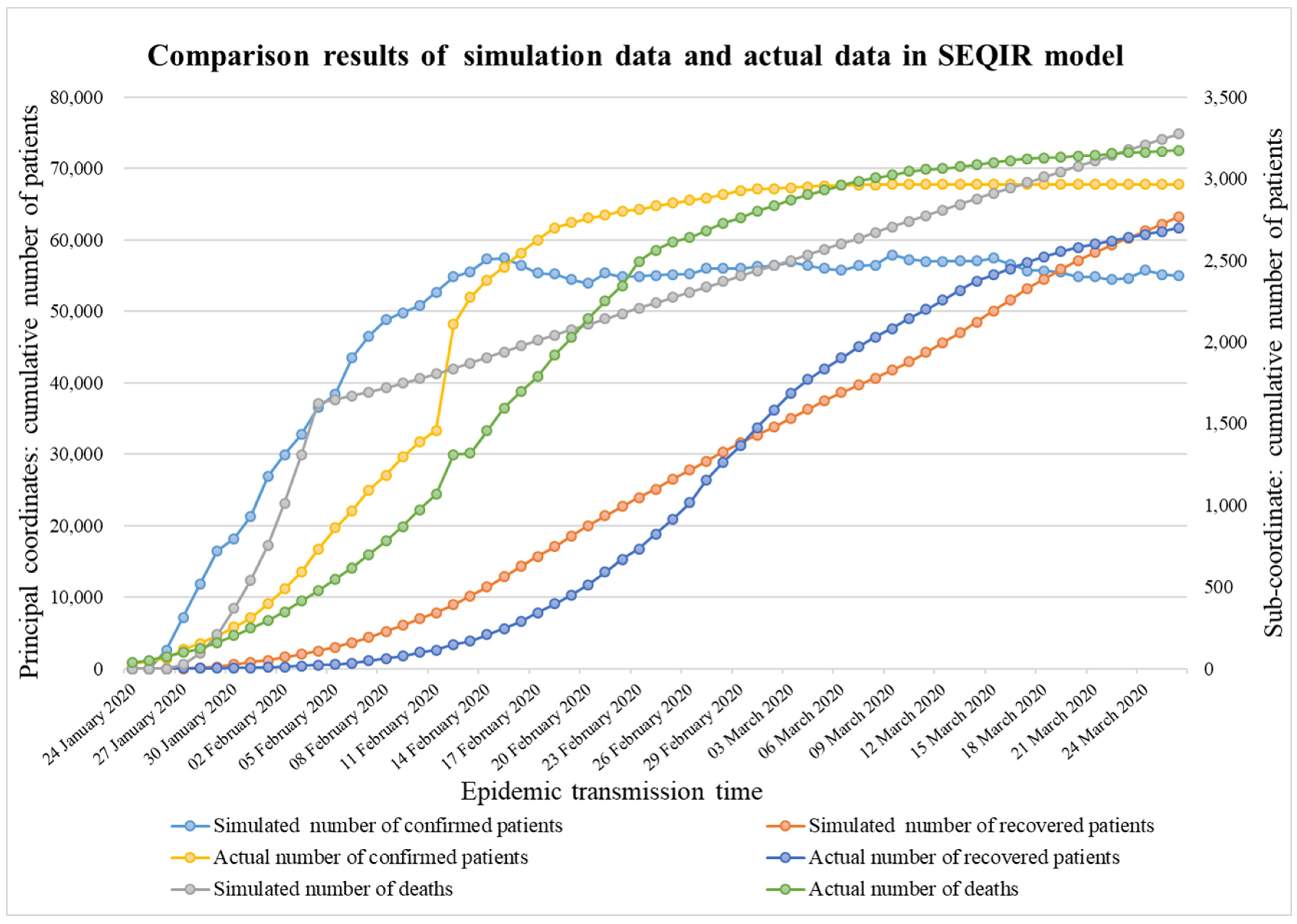
The disease incidence during the outbreak period is simulated using the classic SEIR model, and the simulation results are shown in Figure 7.

As shown in Figure 7, the number of confirmed patients, recovered patients and deaths increased exponentially. The susceptible population is the group with low resistance and susceptibility to disease. Although the number of the susceptible population increased, it is basically stable within a certain range. If no measure is taken after 24 January, the number of confirmed patients will increase exponentially, and prevention and control measures will need to be taken in time to prevent COVID-19 from causing further damage.

Figure 8 shows a comparison of the simulation results with the actual data; during this period, the outbreak mainly occurred in Wuhan City, Hubei Province, China.

Figure 8 shows that the simulated number of patients with confirmed disease follows a trend that is similar to the actual increase. The simulated number of confirmed patients is consistent with the early development of the epidemic, but the actual number of confirmed patients did not reach the simulated level; this was due to our insufficient understanding of the novel coronavirus in the early stage and the lack of medical equipment and experience in detection. This caused the diagnosis to be delayed to a certain degree and resulted in a sudden increase on 17 January.

At present, China’s medical conditions and non-wartime medical supplies are sufficient to permit a maximum response to the epidemic; therefore, the number of cured patients on a daily basis is higher than the simulated result. However, after a certain carrying capacity is exceeded, patients can only be cured under limited conditions, and after 21 January, the number of patients who are cured is lower than the simulated number.

A certain recovery rate is guaranteed, and the mortality rate decreases accordingly. The actual number of deaths after 16 January is lower than the simulated number; this indicates that our medical system can respond in a timely manner to public health emergencies in the early stages and that it can protect our lives and health.

5.2. Control Period

On 23 January, the Chinese government launched a level 1 public health emergency response, suspending the operation of buses, subways, airports and railway stations in Wuhan beginning at 10 a.m. On 24 January, Hubei province launched a level 1 public health emergency response, suspending public transport in other cities.

China has actively taken prevention and control measures against this public health emergency as it enters the prevention and control period. In this paper, the classical SEIR model is improved by adding isolated latent agents to obtain the SEQIR model. The SEQIR model improves the parameters before and after the measure to obtain the improved SEQIR model.

The improved SEQIR model is simulated, and the results are shown in Figure 9.

As shown in Figure 9, the non-susceptible population becomes susceptible through contact with confirmed patients and with patients who are in the incubation period. In the early stage, the number of susceptible patients as the number of confirmed patients increases and then begins to decrease after reaching a peak. The number of confirmed patients increases in the early period and gradually stabilizes in the later period. The number of deaths increases exponentially in the early period and then increases linearly and slowly after 14 February. The number of recovered patients increases linearly after 9 February. The patients in the incubation period show a fluctuating decline and gradually approach the range of 1000–2000. The number of isolated latent patients increases exponentially in the early period and linearly after 17 February.

The experimental results show that after the prevention and control measures are implemented, the increase in the number of confirmed patients flattens out. This illustrates the effectiveness of the control measures that were taken. The period of incubation is affected by the patients because the virus present at each cycle of latency in the human body is different. We need to pay more attention to the patient’s health status in the incubation period; because of improving cure rate for COVID-19, mortality reduces, and the safety of people’s lives is ensured.

A comparison of the simulation results in the control period with the actual data is shown in Figure 10.

Figure 10 shows that the simulated trend in the number of confirmed patients is consistent with the actual data, but the number of patients from 24 January to 16 February in the actual data is lower than the simulated number; this is in Wuhan city, after being sealed off, and the limitations of medical resources caused the actual number of confirmed patients to be higher than the simulated number. The later simulated data show a decline after the peak, whereas the number of confirmed patients shows no sharp decline and basic stability. The trends in the variation in the number of simulated and actually cured people are basically the same, the difference between the results is small, and the simulation effect is satisfactory.

The simulated number of deaths increased exponentially in the early period and linearly after 3 February, while the actual death toll showed an “S-shaped” increase. Although the simulated results are somewhat different from the actual data, it is necessary to further study the changing trend of the death toll and to modify the parameters related to the death toll in the model. In this stage, the simulation results for the number of confirmed patients and recovered patients are good, but the change in the number of deaths needs to be further improved.

The outbreak period simulated by using the classic SEIR model and parameters with only a single rate does not correspond to the changing situation of the transmission of the epidemic. The results of the simulation using the improved SEQIR model are closer to reality, so the predicted data of the classic SEIR model is compared with the simulation results of the improved SEQIR model from 24 January to 19 April, and the results of the comparison are shown in Figure 11, Figure 12, Figure 13 and Figure 14.

Although during the outbreak period the number of confirmed patients shows exponential growth, the parameters related to the explosion rate are fixed, which is not in conformity with the spread of the epidemic. As Figure 11 shows, in the control period, the predicted data appears as a smooth increasing trend, but the simulation number of confirmed patients presents a mass increase at first and then levels off. This is due to the prevention and control measures having a time lag, and not working right away; however, the subsequent flat growth proved the effectiveness of the control measures, as there is no large-scale exponential growth from 14 February to 26 March. By comparing the predicted results and the simulation results in the control period, it can be found that the improved SEQIR model more accurately describes the transmission situation of the epidemic from 24 January to 26 March, indicating that the effect of our phased study is better.

As shown in Figure 12, during the control period the cure rate increased as the corresponding policies took effect, causing the number of recovered patients to present linear growth and to far better predict the number of recovered patients. This is what we hoped to see. The effect of the prevention and control measures on the number of recovered patients is more consistent with the actual data, and thus, the improved SEQIR model is effective.

Figure 13 shows that the number of deaths during the outbreak period shows a growth in the index level, and a continuation of this trend will result in massive deaths—an outcome that we do not wish to see. We cannot allow this type of situation to develop. Following the implementation of prevention and control measures, there is a time lag before the improvement in the death toll from the control period, and the number of deaths increased rapidly to approximately 1800. With the improved SEQIR model, which corrected the mortality rate and the recovery rate, the increase in the number of deaths was limited to a certain rate and began to increase slowly.

Although the effect of the death toll during the prevention and control period is better than that predicted during the outbreak period, there is still a gap between the simulation results and the actual data. Thus, further adjustment of the model is required to get closer to the change in the death toll during the prevention and control period.

As shown in Figure 14, the number of patients with isolation latency increased slowly from 24 January to 19 February. Because it takes a certain amount of time to check the close contacts of the confirmed patients and the initial isolation measures are not perfect [31], the number of patients with isolation latency increased slowly. After 19 February, there was a linear increase, and after the number of confirmed patients reached a plateau, the isolation measures continued, and the number of patients in the incubation period of isolation continued to increase.

Based on the above comparisons, it is feasible and effective for us to divide the epidemic transmission periods into the outbreak period and the control period, and the model is improved according to the characteristics of each period. The improved effect is consistent with the actual data, and the simulation results effect of the improved SEQIR model in the control period is better than that predicted data of the classical SEIR model, proving the effectiveness of the improved SEQIR model.

5.3. Steady Period

After a period of reaction, the epidemic spreading conditions in China are effectively controlled, and the focus began to shift to the number of new patients according to the SEQIR Ⅱ model in the steady period. A comparison of the new patients by the simulation results with the actual data, is shown in Figure 15.

(Special note: the epidemic data reported by the Wuhan Municipal Health Commission was revised up to 24:00 on 16 April 2020 according to law, and the outlier values on 16 April did not change the overall effect of the model.)

As Figure 15 shows, the simulated number of new patients fluctuated and decreased rapidly. Compared with the actual number of new patients, it basically remained at the single-digit level, indicating that the actual control situation was better than the simulated one. However, the rapid decline in the simulated number of new patients also indicated the effectiveness of the prevention and control measures.

The simulated number of recovered patients decreased with the decrease in the actual number of confirmed patients, showing a linear and stable decline, but the actual number of recovered patients decreased rapidly after the peak, and it fluctuated. The comparison shows that the number of medically recovered patients has a certain limit and that the simulation can be very close to the actual change trend but cannot fully fit it. The number of simulated deaths and the actual number of deaths are similar.

6. Conclusions and Discussion

The COVID-19 pandemic will not only be a threat to life and health, but also results in economic losses and hinders social security and national development. In this paper, by establishing a multistage time-delay control model (MTCM) for COVID-19 to analyze the spread of the epidemic in three periods, the results were as follows:

During the outbreak period of the epidemic, the classic SEIR model can well reveal the conditions, and according to this trend, the outbreak will show an exponential increase. The number of the susceptible population increased, but it is basically stable within a certain range. The result of the simulated number of confirmed patients is consistent with the early development of the epidemic, but the actual number of confirmed patients did not reach the simulated level. It is clear that our insufficient understanding of the novel coronavirus in the early stage and the lack of medical equipment and experience in detection are important to correctly interpret the results.

During the control period, according to the national relevant measures, effective contact numbers, infection rates, cure rates, mortality and other influencing factors are included to improve the SEQIR model. The improved SEQIR model makes it more adaptable to characteristics and the actual data in the control period. The experimental results show that the number of confirmed patients flattens out after the prevention and control measures. This illustrates the effectiveness of the control measures that were taken. It is important to note that the simulated number of confirmed patients is consistent with the actual data, but the actual data is less than it is from 24 January to 16 February. The reason is the limitations of medical resources in Wuhan city after being sealed off.

After a period of prevention and control, the epidemic has been controlled and enters the steady period. At this time, the SEQIR Ⅱ model is used to study the changes of the new data, the influencing factors of the population moving in and out are added, patients are divided into symptomatic patients and asymptomatic patients, and the simulation experiment results are conducted to compare the actual data. The poor simulation effect of the number of recovered patients indicates that the model still has defects in this aspect.

The simulation experimental results show that the MTCM explains the evolution of the epidemic and changing situation well. This should help us later in developing public health emergency response measures and in research on similar situations.

In future work, the following aspects will be further studied:

• For the comparison between the predicted data of the classical SEIR model and the simulated data of the improved SEQIR model for the control period, the actual data is not added for discussion, which needs to be improved later.
• Changes in mortality in the improved SEQIR model will be modified to make it more consistent with changes in the number of deaths during the control period.
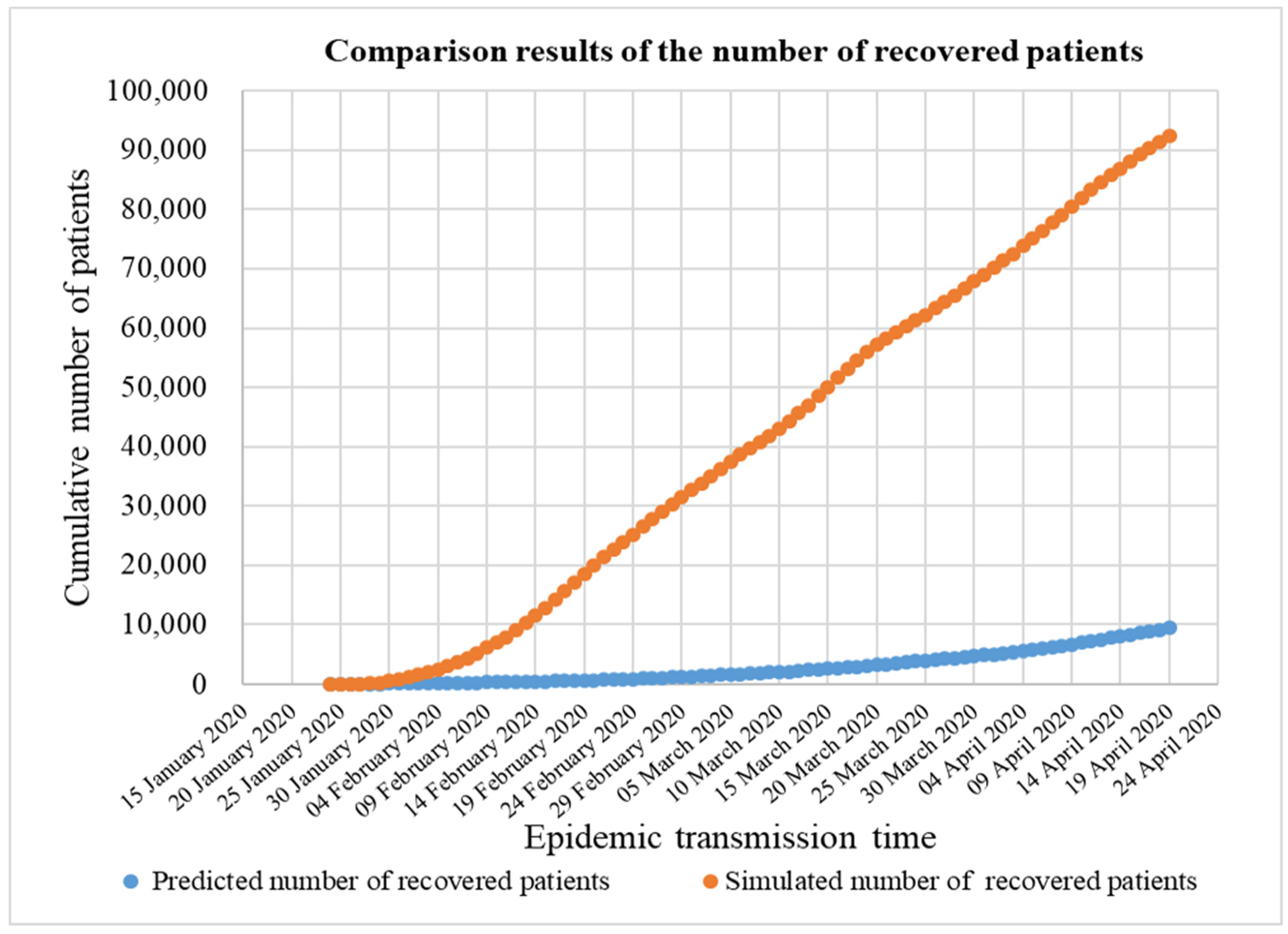
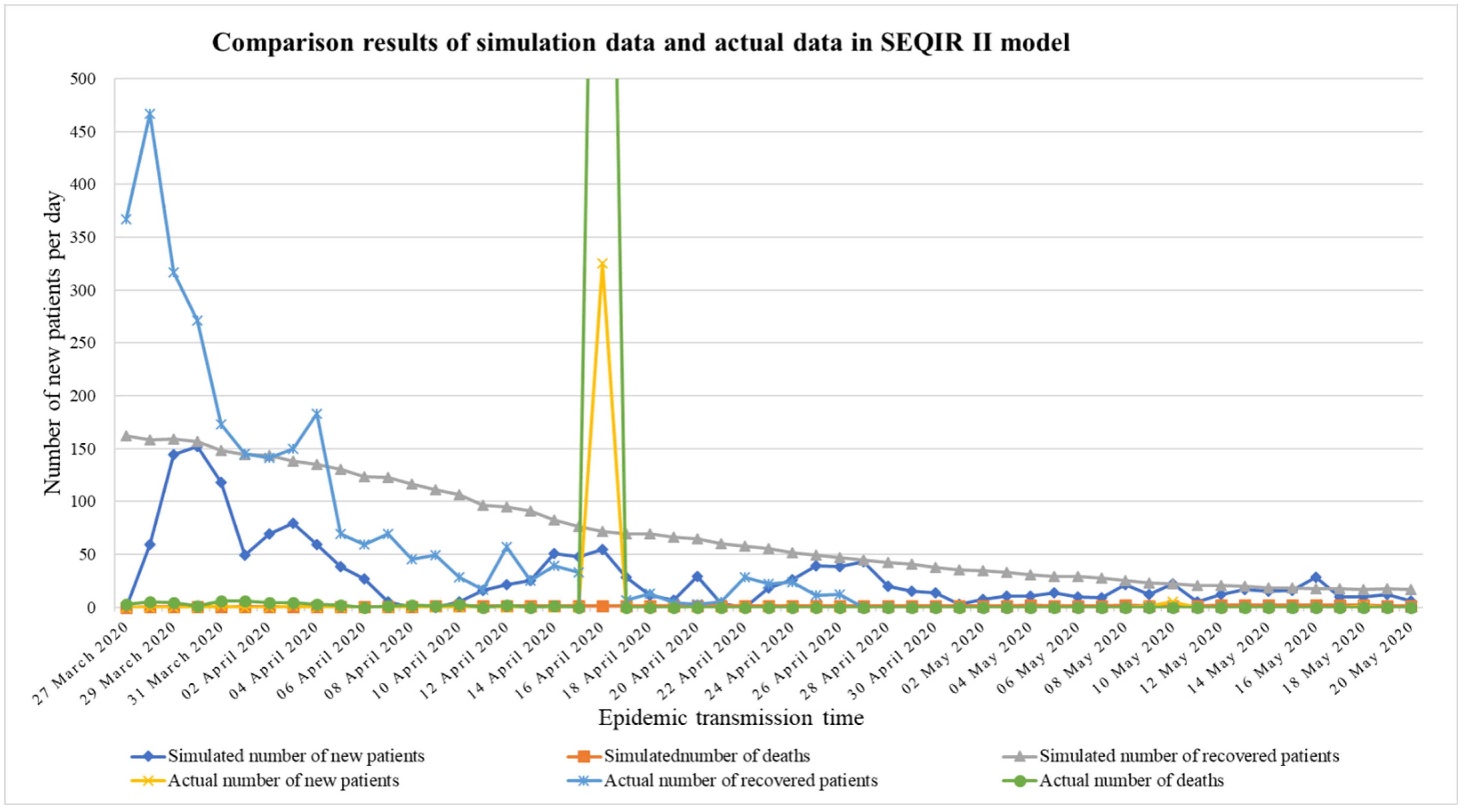
• This may alter or improve aspects of the SEQIR Ⅱ model, in which the simulation effect of the number of recovered patients is poor.
• The SEQIR Ⅱ model will be modified to better simulate the process of a sudden and rapid decline in the number of recovered patients.

The MTCM should be adjusted to better simulate real changes and put forward better policies and measures to prevent and control the spread of COVID-19 in light of the current situation. The goal is to win this war on human security with minimal damage.

References

1. Kumar, P.; Morawska, L. Could fighting airborne transmission be the next line of defence against COVID-19 spread? City Environ. Interact. 2019, 4, 100033. [Google Scholar] [CrossRef] [PubMed]
2. Shuai, Y.; Jiang, C.; Su, X.; Yuan, C.; Huang, X. A Hybrid Clustering Model for Analyzing COVID-19 National Prevention and Control Strategy. In Proceedings of the 2020 IEEE 6th International Conference on Control Science and Systems Engineering (ICCSSE), Beijing, China, 17–19 July 2020. [Google Scholar] [CrossRef]
3. Spaan, W.; Cavanagh, D.; Horzinek, M.C. Coronaviruses: Structure and genome expression. J. Gen. Virol. 1988, 69 Pt 12, 2939–2952. [Google Scholar] [CrossRef]
4. Zhu, N.; Zhang, D.; Wang, W.; Li, X.; Yang, B.; Song, J.; Zhao, X.; Huang, B.; Shi, W.; Lu, R.; et al. A Novel Coronavirus from Patients with Pneumonia in China, 2019. N. Engl. J. Med. 2020, 382, 727–733. [Google Scholar] [CrossRef] [PubMed]
5. Chen, Y.; Liu, Q.; Guo, D. Emerging coronaviruses: Genome structure, replication, and pathogenesis. J. Med. Virol. 2020, 92, 418–423. [Google Scholar] [CrossRef] [PubMed] [Green Version]
6. Prasse, B.; Achterberg, M.A.; Ma, L.; van Mieghem, P. Network-Based Prediction of the 2019-nCoV Epidemic Outbreak in the Chinese Province Hubei. Appl. Netw. Sci. 2020, 5, 1–11. [Google Scholar]
7. Wang, D.; Tan, D.; Lei, L. Particle swarm optimization algorithm: An overview. Soft Comput. 2018, 22, 387–408. [Google Scholar] [CrossRef]
8. He, S.; Banerjee, S. Epidemic outbreaks and its control using a fractional order model with seasonality and stochastic infection. Phys. A Stat. Mech. Its Appl. 2018, 501, 408–417. [Google Scholar] [CrossRef]
9. Mei, W.; Liu, Z.; Zhu, J.; Du, L. Extreme IR Model for COVID-19 Real-Time Forecasting. J. Univ. Electron. Sci. Technol. China 2020, 49, 362–368. [Google Scholar] [CrossRef]
10. Law, K.B.; Peariasamy, K.M.; Gill, B.S.; Singh, S.; Sundram, B.M.; Rajendran, K.; Dass, S.C.; Lee, Y.L.; Goh, P.P.; Ibrahim, H.; et al. Tracking the early depleting transmission dynamics of COVID-19 with a time-varying SIR model. Sci. Rep. 2020, 10, 21721. [Google Scholar] [CrossRef]
11. Santos, I.D.; Almeida, G.; Moura, F.D. Adaptive SIR model for propagation of SARS-CoV-2 in Brazil. Phys. A Stat. Mech. Its Appl. 2021, 569, 125773. [Google Scholar] [CrossRef]
12. Guerrero-Nancuante, C.; Manriquez, R. An epidemiological forecast of COVID-19 in Chile based on the generalized SEIR model and the concept of recovered. Medwave 2020, 20, e7898. [Google Scholar] [CrossRef] [PubMed]
13. Wu, J.T.; Kathy, L.; Leung, G.M. Nowcasting and forecasting the potential domestic and international spread of the 2019-nCoV outbreak originating in Wuhan, China: A modelling study. Lancet 2020, 395, 689–697. [Google Scholar] [CrossRef] [Green Version]
14. Yang, Z.; Zeng, Z.; Wang, K.; Wong, S.-S.; Liang, W.; Zanin, M.; Liu, P.; Cao, X.; Gao, Z.; Mai, Z.; et al. Modified SEIR and AI prediction of the epidemics trend of COVID-19 in China under public health interventionsy. J. Thorac. Dis. 2020, 12, 165–174. [Google Scholar] [CrossRef] [PubMed]
15. Walker, P.G.T.; Whittaker, C.; Watson, O.; Baguelin, M.; Ainslie, K.E.C.; Bhatia, S.; Bhatt, S.; Boonyasiri, A.; Boyd, O.; Cattarino, L.; et al. Report 12: The Global Impact of COVID-19 and Strategies for Mitigation and Suppression; Imperial College London: London, UK, 2020. [Google Scholar]
16. Driessche, P.; Watmough, J. A simple SIS epidemic model with a backward bifurcation. J. Math. Biol. 2000, 40, 525–540. [Google Scholar] [CrossRef] [PubMed]
17. Cai, Y.; Kang, Y.; Wang, W. A stochastic SIRS epidemic model with nonlinear incidence rate. Appl. Math. Comput. 2017, 305, 221–240. [Google Scholar] [CrossRef] [Green Version]
18. Chen, Y.C.; Lu, P.E.; Chang, C.S.; Liu, T.H. A Time-dependent SIR model for COVID-19. IEEE Trans. Netw. Sci. Eng. 2020, 7, 3279–3294. [Google Scholar] [CrossRef]
19. Guo, W.; Xu, T.; Tang, K.M. Mestimator based online sequential extreme learning machine for predicting chatic time series with outilters. Neural Comput. Appl. 2017, 2017, 4093–4110. [Google Scholar] [CrossRef]
20. Du, Z.; Wang, L.; Cauchemez, S.; Xu, X.; Wang, X.; Cowling, B.J.; Meyers, L.A. Risk for Transportation of 2019 Novel Coronavirus (COVID-19) from Wuhan to Cities in China. Emerg. Infect. Dis. 2020, 26, 1049–1052. [Google Scholar] [CrossRef] [Green Version]
21. Boldog, P.; Tekeli, T.; Vizi, Z.; Dénes, A.; Bartha, F.A.; Röst, G. Risk assessment of novel coronavirus COVID-19 outbreaks outside China. J. Clin. Med. 2020, 9, 571. [Google Scholar] [CrossRef] [Green Version]
22. Dong, E.; Du, H.; Gardner, L.M. An interactive web-based dashboard to track COVID-19 in real time. Appl. Math. Comput. 2017, 305, 221–240. [Google Scholar] [CrossRef]
23. Gill, B.S.; Jayaraj, V.J.; Singh, S.; Mohd Ghazali, S.; Cheong, Y.L.; Md Iderus, N.H.; Sundram, B.M.; Aris, T.B.; Mohd Ibrahim, H.; Hong, B.H.; et al. Modelling the Effectiveness of Epidemic Control Measures in Preventing the Transmission of COVID-19 in Malaysia. Int. J. Environ. Res. Public Health 2020, 17, 5509. [Google Scholar] [CrossRef] [PubMed]
24. Kock, R.A.; Karesh, W.B.; Veas, F.; Velavan, T.P.; Simons, D.; Mboera, L.E.G.; Dar, O.; Arruda, L.B.; Zumla, A. 2019-nCoV in context: Lessons learned? Lancet Planet. Health 2020, 4, e87–e88. [Google Scholar] [CrossRef] [Green Version]
25. Mat, N.F.C.; Edinur, H.A.; Razab, M.K.A.A.; Safuan, S. A Single Mass Gathering Resulted in Massive Transmission of COVID-19 Infections in Malaysia with Further International Spread. J. Travel Med. 2020, 27, taaa059. [Google Scholar] [CrossRef] [PubMed]
26. Fanelli, D.; Piazza, F. Analysis and forecast of COVID-19 spreading in China, Italy and France. Chaos Solitons Fractals 2020, 134, 109761. [Google Scholar] [CrossRef]
27. Li, Q.; Guan, X.; Wu, P.; Wang, X.; Zhou, L.; Tong, Y.; Ren, R.; Leung, K.; Lau, E.H.Y.; Wong, J.Y.; et al. Early transmission dynamics in Wuhan, China, of novel coronavirus–infected pneumonia. N. Engl. J. Med. 2020, 382, 1199–1207. [Google Scholar] [CrossRef]
28. Keeling, M.J.; Eames, K. Networks and epidemic models. J. R. Soc. Interface 2005, 2, 295–307. [Google Scholar] [CrossRef] [Green Version]
29. Zhuang, Z.; Zhao, S.; Lin, Q.; Cao, P.; Lou, Y.; Yang, L.; Yang, S.; He, D. Preliminary estimating the reproduction number of the coronavirus disease (COVID-19) outbreak in Republic of Korea from 31 January to 1 March 2020. Int. J. Infect. Diseases 2020, 95, 308–310. [Google Scholar] [CrossRef]
30. Keeling, M.J.; Danon, L. Mathematical modelling of infectious diseases. Br. Med. Bull. 2009, 92, 33–42. [Google Scholar] [CrossRef]
31. Tang, B.; Wang, X.; Li, Q.; Bragazzi, N.L.; Tang, S.; Xiao, Y.; Wu, J. Estimation of the Transmission Risk of the 2019-nCoV and Its Implication for Public Health Interventions. J. Clin. Med. 2020, 9, 462. [Google Scholar] [CrossRef]
Figure 1. Classical SEIR model diagram for the outbreak period.
Sustainability 14 14657 g001
Figure 2. SEIR model diagram for the outbreak period (no measure intervention).
Sustainability 14 14657 g002
Figure 3. Improved SEQIR model diagram for the control period.
Sustainability 14 14657 g003
Figure 4. The improved SEQIR model diagram for the control period (effective isolation measures).
Sustainability 14 14657 g004
Figure 5. SEQIR II model diagram for the steady period.
Sustainability 14 14657 g005
Figure 6. SEQIR Ⅱ model diagram for the steady period (migration and emigration populations, the confirmed patients who are symptomatic and asymptomatic patients).
Sustainability 14 14657 g006
Figure 7. Classic SEIR model simulation of the outbreak period.
Sustainability 14 14657 g007
Figure 8. Comparison of classical SEIR model of the actual data with simulation results.
Sustainability 14 14657 g008
Figure 9. Improved SEQIR model simulation results.
Sustainability 14 14657 g009
Figure 10. Comparison of the actual data with the simulated results in the improved SEQIR model.
Sustainability 14 14657 g010
Figure 11. Comparison of the number of confirmed patients.
Sustainability 14 14657 g011
Figure 12. Comparison of the number of recovered patients.
Sustainability 14 14657 g012
Figure 13. Comparison of patient deaths.
Sustainability 14 14657 g013
Figure 14. The number of patients with isolation latency.
Sustainability 14 14657 g014
Figure 15. Comparison of the actual data with simulation results in the SEQIR II model.
Sustainability 14 14657 g015