Economic and Environmental Evaluation of a Single-Story Steel Building in Its Life Cycle: A Comprehensive Analysis

Abstract

In this study, the possibility of applying the Life Cycle Thinking approach to structural design, considering all aspects and phases of the structure’s life, is investigated. The idea is to develop a procedure for the analysis of the economic and environmental impacts of structures in their life cycle, including not only ordinary costs along life cycle phases but also the extraordinary costs resulting from damage and anticipated end-of-life caused by unexpected natural hazards. The building performance under extraordinary conditions is calculated according to a time-based Loss Assessment Analysis. Such analysis provides the probable performance of a building and its components over a given period of time, considering all the hazardous events that can occur in that period, the probability of occurrence of each event, and the related effects. The outlined approach is applied to a case study of a single-story steel office building located in Italy. Two LC scenarios, having a duration of 2 years and 50 years, are considered. Results show that contributions of environmental impacts and benefits related to end-of-life management and economic losses for natural hazards are significant and not negligible. It is highlighted that the greatest challenge faced when using such a comprehensive approach is represented by data availability and representativeness that deeply limits the possibility of its implementation.

1. Introduction

Life Cycle Thinking (LCT) is a holistic approach that brings great innovations in the design of products and processes. Taking an LCT approach means considering products and processes over their entire life, from conception to production processes, use, and disposal. One of the main tools of LCT is the so-called Life Cycle Assessment (LCA) [1].

The LCT approach has implications in many fields of our life of an economic, environmental, and social nature. In some fields, such as the production of automobiles [2], it has been implemented for a long time. In other fields, it is more recent, and it is struggling to be upheld. The reason is mainly economic: some products have life cycles much longer than others [3], and too-long life cycles are hardly compatible with market trends, which have very tight return times.

The role of the life cycle length of products in LCT is evident in the building sector [4,5,6,7]. A construction is a system composed of multiple components. Some of them have relatively short life cycles (windows, systems, etc.), both because they are more subject to wear and tear and because, being less expensive, they are more subject to changes in people needs and trends. Others, such as structures, have longer life cycles, both because they are normally less subject to wear and tear and because interventions on them are more expensive [8].

For this reason, the LCT approach in the construction sector is currently mainly applied to the analysis and design of short-life components. Great importance is given to the design of technical and cladding systems to improve energy efficiency, with the aim of reducing the economic and environmental costs of building heating/cooling. Past studies have indeed shown that usually, the use phase (related to operational energy consumption) presents the highest environmental impacts (62–98% of total life cycle impacts at the entire building level), while the construction phase (related to embodied energy consumption) accounts for 1–20% only [9].

However, economic, environmental, and social demands increasingly require dealing with components with a longer life cycle, such as structures. In buildings, not only do structures embody energy during manufacturing, construction, and end of life, but also during the use stage. Normally undervalued, such a stage may generate substantial impacts related to material degradation (implying cyclically revising the coatings of steel structures or protecting the reinforcements of concrete structures) and to structural damage that may result from extraordinary events (earthquakes, floods, fires, etc.). Such structural damage may or may not occur in the life of the structure, but when it occurs, it has devastating social, economic, and environmental impacts. It involves costs associated with either repair or anticipated end of life, and, on the other hand, it generates environmental impacts caused by recovery operations or substitutions. For this reason, the application of LCT to buildings’ structures implies considering both ordinary and extraordinary events that may occur in their life through a suitable probabilistic approach [10].

The application of LCT to structures and related components has already been tested at various levels. Some recently published studies have tried to integrate the classical LCT approach, related to the ordinary life of structures, with the impacts related to natural hazards [11]. In certain cases, various aspects of the integration of risk assessment procedures in the ecological sustainability of buildings have been explored [12]. In [13], a method for combining the results obtained from an LCA and earthquake damage assessment for buildings is presented and used to make a direct comparison of steel and concrete as materials. However, in all these studies, strong assumptions not directly related to the physical damage mechanism caused by the hazard have been made to calculate environmental impacts.

Thus, the literature review shows a general lack of a comprehensive methodology that systematically addresses the potentially significant variables affecting the life cycle of buildings and infrastructures, and that relies on already well-consolidated techniques of stochastic engineering and costs and environmental impact assessment.

In this study, the possibility of applying the LCT approach to structural design, considering all aspects and phases of the structure’s life, is investigated. The idea is to develop a procedure for the analysis of the economic and environmental performance of structures in their life cycle, including not only ordinary costs along life cycle phases, but also the extraordinary costs resulting from damage and anticipated end-of-life caused by unexpected natural hazards with the probabilistic Loss Assessment Analysis (LAA) developed in the field of risk engineering [12,14,15,16,17].

Specifically, considering a one-story steel office building as a case study, the purposes of this study are:

-

Develop a reliable methodology to evaluate the economic and environmental performance of a building or building components along the lifetime, considering not only ordinary events (construction, demolition at the end-of-life cycle) but also extraordinary events that can occur along the life cycle of a building;

-

Evaluate the applicability of this tool in relation to the data currently available.

The integration of such approaches can lead to a deeper and more comprehensive evaluation of the overall building performance, supporting the decision-making at the design stage and improving the overall environmental and economic sustainability.

2. Methodology

The methodology proposed is based on the idea that the performance ${\mathrm{X}}_{\mathrm{LC}}$ of a building along its Life Cycle (LC) in terms of either economic costs or environmental impacts can be evaluated as given by Equation (1):

$${\mathrm{X}}_{\mathrm{LC}}{=\mathrm{X}}_{\mathrm{ord},\mathrm{LC}}{+\mathrm{X}}_{\mathrm{ext},\mathrm{LC}}$$

(1)

where ${\mathrm{X}}_{\mathrm{ord},\mathrm{LC}}$ and ${\mathrm{X}}_{\mathrm{ext},\mathrm{LC}}$ are the costs/impacts related to the building performance under ordinary and extraordinary actions, respectively.

${\mathrm{X}}_{\mathrm{ord},\mathrm{LC}}$ is evaluated as the sum of the costs/impacts related to each $\mathrm{ith}$ building component along building life cycle phases and does not vary with the duration Y_LC of the LC, as specifically given by Equation (2):

$${\mathrm{X}}_{\mathrm{ord},\mathrm{LC}}={\displaystyle \sum }_{\mathrm{i}}\left({\mathrm{X}}_{\mathrm{ord},\mathrm{c},\mathrm{i}}{+\mathrm{X}}_{\mathrm{ord},\mathrm{o},\mathrm{i}}{+\mathrm{X}}_{\mathrm{ord},\mathrm{m},\mathrm{i}}{+\mathrm{X}}_{\mathrm{ord},\mathrm{e},\mathrm{i}}\right)$$

(2)

where ${\mathrm{X}}_{\mathrm{ord},\mathrm{c},\mathrm{i}}$,${\mathrm{X}}_{\mathrm{ord},\mathrm{o},\mathrm{i}}$ ${\mathrm{X}}_{\mathrm{ord},\mathrm{m},\mathrm{i}}$, and ${\mathrm{X}}_{\mathrm{ord},\mathrm{e},\mathrm{i}}$ are the construction, operation, maintenance, and end-of-life costs/impacts respectively, evaluated deterministically according to best available information for the specific case (material, transportation and installation costs, end of life management costs, benefits for reusing, recycling, etc.).

The building performance under extraordinary conditions ${\mathrm{X}}_{\mathrm{ext},\mathrm{LC}}$ is calculated according to a time-based LAA. Such analysis provides the probable performance of a building and its components over a given period of time [18], considering all the hazardous events that can occur in that period, the probability of occurrence of each event, and the related effects (e.g., costs for substitution or restoration of damaged components, indirect costs for the loss of building functionality; environmental impacts generated by energy consumption and material consumption required for restoration or substitution, etc.).

Specifically, considering the effects caused by the expected $\mathrm{jth}$ hazard on each $\mathrm{ith}$ building component, ${\mathrm{X}}_{\mathrm{ext},\mathrm{LC}}$ is given by Equation (3):

$${\mathrm{X}}_{\mathrm{ext},\mathrm{LC}}={\displaystyle \sum }_{\mathrm{j}}{\displaystyle \sum }_{\mathrm{i}}{\displaystyle \int }{\mathsf{\lambda }}_{\mathrm{i},\mathrm{j}}\left[\mathrm{DV}\right|\mathrm{LC}]\mathrm{dDV}$$

(3)

where ${\mathsf{\lambda }}_{\mathrm{i},\mathrm{j}}\left[\mathrm{DV}\right|\mathrm{LC}]$ is the probability of exceeding a Decision Variable (DV) (i.e., the repair cost of the $\mathrm{ith}$ component) within LC duration for different levels of Intensity Measure (IM) selected to describe the $\mathrm{jth}$ hazard. Following the basic mathematical approach given by the Pacific Earthquake Engineering Research Center [19], ${\mathsf{\lambda }}_{\mathrm{i},\mathrm{j}}\left[\mathrm{DV}\right|\mathrm{LC}]$ can be expressed by Equation (4):

$${\mathsf{\lambda }}_{\mathrm{i},\mathrm{j}}\left[\mathrm{DV}\right|\mathrm{LC}]={\displaystyle \int }{\displaystyle \int }{\displaystyle \int }{(\mathrm{p}\left[\mathrm{DS}\right]·\mathrm{p}\left[\mathrm{EDP}\right]·\mathrm{p}\left[\mathrm{IM}\right])}_{\mathrm{i}}·{\mathsf{\lambda }}_{\mathrm{j}}\left[\mathrm{IM}\right]\mathrm{dIM}\mathrm{dEDP}\mathrm{dDS}$$

(4)

The probability distribution of likely economic/environmental effects DV is thus conditioned on the expected Damage State (DS) of the components of the building experiencing certain Engineering Demand Parameter (EDP) for a given intensity level IM with a corresponding probability of exceedance λ [IM] in LC duration [19].

To define the probability of exceedance ${\mathsf{\lambda }}_{\mathrm{j}}\left[\mathrm{IM}\right]$ of a given intensity IM of the $\mathrm{jth}$ hazard at the building’s site, a hazard analysis is required. The intensity parameter IM shall be related to the structural behavior or structural response of the building (e.g., spectral acceleration for seismic hazard). The range of hazard intensities of interest can be selected on a case by case, depending on the site and on the scope of the study.

The probabilistic distribution $\mathrm{p}$ of EDPs, associated with given intensity measures IM of the action ($\mathrm{p}\left[\mathrm{IM}\right])$ can be obtained through a set of structural analyses, based on the non-linear modeling of the structure and on the evaluation of its structural response in terms of EDPs (e.g., floor acceleration, inter-story drift, top displacement, etc.) under the actions estimated through the hazard analysis.

The probabilistic distribution $p$ of the likely damage DS related to EDPs $(\mathrm{p}\left[\mathrm{EDP}\right])$ is defined through fragility functions, indicating the conditional probability of incurring a damaged state given a value of demand [18]. Fragility functions for building components are usually available for different damage state thresholds to identify the extent of repair required to restore the building to the undamaged state.

Finally, the probabilistic distribution $\mathrm{p}$ of the decision variable DV given the expected damage $\mathrm{DS}$ ($\mathrm{p}\left[\mathrm{DS}\right]$) is defined through consequence functions, providing the likely consequences of damage translated into potential repair and replacement costs, repair time, casualties, unsafe placarding, and other impacts [18].

Depending on the aim of the analysis, different decision variables DV may be chosen. In particular:

-

If the aim of the analysis is to evaluate the overall economic costs of the building along its LC (${\mathrm{X}}_{\mathrm{LC}}{=\mathrm{C}}_{\mathrm{LC}}$), the decision variable adopted in the LAA will be the sum of direct and indirect economic costs related to the impacts of the hazard on the building (reparation/replacement costs, use interruption costs, etc.);

-

If the aim of the analysis is to evaluate the environmental impacts of the building along its LC (${\mathrm{X}}_{\mathrm{LC}}{=\mathrm{E}}_{\mathrm{LC}}$), different decision variables may be adopted, such as Global Warming Potential (GWP), measured in terms of Greenhouse Gas (GHG) emissions, Embodied Energy, CO₂ emissions, etc. Whatever the choice, the environmental impacts include the effects of extraordinary events on the building (e.g., GHG produced by the replacement/repair of components, etc.).

It is worth noting that the application of the methodology requires the definition of the LC scenario. The LC scenario definition consists of setting the LC duration ${\mathrm{Y}}_{\mathrm{LC}}$, the operational phase of the building, the operation and maintenance plan, and the end-of-life management. Moreover, it identifies the hazards to characterize extraordinary actions.

3. Case Study

3.1. Description of the Building

The case study considered is a simple one-story steel office building specially designed for testing the methodology. Both structural (columns and beams) and non-structural elements (external cladding system) are considered in the study. The systems of the building (electric, heating, and air conditioning) are not considered.

The structural design solutions are developed according to the Italian Code [20], and the instructions for wind actions on structures [21] and Eurocode 3 [22] are adopted on a voluntary base when not in contrast with the Italian Standard. Structural design has been carried out, pushing work rates up to 90% to highly exploit members’ capacity.

The building is in the Liguria region (Italy), in Ortonovo, close to the river Parmignola, at an altitude of 19 m a.s.l. The shape of the building is approximately rectangular: it has eight 5.3 m spans in the longitudinal direction and three spans in the transversal one, for a total width of 25 m. The roof is a duo pitch, with an inclination of around 9°; the maximum height of the building is 6 m (Figure 1).

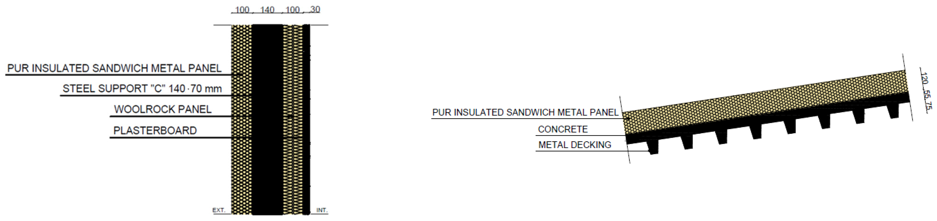
The cladding system for external walls is composed of polyurethane panels, supported by a cold-formed steel stud, rock-wool panels, and a layer of plasterboard; the roof cladding system is a 12 cm commercial double skin panel insulated with polyurethane foam (Figure 2). Connections between panels and structure are rigid, according to the definition given by the Italian Building Code [20], and they are considered screwed to the metal studs [23].

3.2. Life Cycle Scenario Definition

Two LC scenarios (namely LC₂ and LC₅₀) are considered for the case study. They have a duration of 2 years and 50 years, respectively, due to the following reasons:

-

A 2-year LC duration (YLC = 2) allows foreseeing the features of the end-of-life scenario more reliably (i.e., estimation of demolition and material disposal costs). This scenario is representative in case the building is designed for short time use, associated with one-time events (temporary exhibitions, etc.);

-

A 50-year LC duration (YLC = 50) is the standard nominal life of ordinary buildings adopted in both structural design and LCAs of buildings.

The LC scenarios cover the construction phase, according to current practice, and the end-of-life phase, foreseeing mechanical demolition performed with excavators, hydraulic shears, bulldozers, and recovery of building materials. Specifically, at the end of life, it is assumed that structural steel is recycled, wool rock and plasterboard are disposed of in landfills, and sandwich polyurethane panels are separated to recycle the steel layers. Operational phase and maintenance operations are disregarded; as for maintenance, this assumption also accounts for the fact that the ordinary lifespan of structural and non-structural is longer than Y_LC in both scenarios. Finally, earthquakes and floods are the hazards considered in both LC scenarios.

3.3. Assessment of the Performance under Ordinary Conditions

3.3.1. Economic Costs

When economic costs are considered, Equation (2) can be re-written in the following form:

$${\mathrm{C}}_{\mathrm{ord},\mathrm{LC}}={\displaystyle \sum }_{\mathrm{i}}\left({\mathrm{C}}_{\mathrm{ord},\mathrm{c},\mathrm{i}}+{\mathrm{C}}_{\mathrm{ord},\mathrm{o},\mathrm{i}}{+\mathrm{C}}_{\mathrm{ord},\mathrm{m},\mathrm{i}}+{\mathrm{C}}_{\mathrm{ord},\mathrm{e},\mathrm{i}}\right)$$

(5)

Estimation of economic costs during the construction phase ${\mathrm{C}}_{\mathrm{ord},\mathrm{c}}$ is carried out according to the current practice through a bill of quantities. The cost of each single ith component is estimated by applying the unitary cost reported in the Prices List of building works [24,25,26] to the total quantity of components or installation. The unitary cost reported accounts for the costs of all necessary resources (workers, materials, and machines utilized); prices refer to standard elements and installation operations and include shares of general expense and profit for the construction company. When a component or an installation operation is not reported within the Prices List (e.g., it is non-standard), the estimation of unitary price is developed through a “price analysis”. This method consists of assessing—for a single unit of component or installation work—the necessary resources in terms of materials, machinery, and labor force. For example, for the supply of a non-standard steel component, the cost is given by raw material cost, workers cost hires of the necessary machinery, transport from the workshop to the construction site, general expenses, and profit of the construction company.

Based on the considered LC scenario and in relation to the life span of the structural and external cladding components, which is higher than the time intervals considered in the evaluation (2 and 50 years), the economic costs for operation and maintenance ${\mathrm{C}}_{\mathrm{ord},\mathrm{o}}$ and ${\mathrm{C}}_{\mathrm{ord},\mathrm{m}}$ can be considered equal to zero. The calculation of economic costs during the end-of-life phase ${\mathrm{C}}_{\mathrm{ord},\mathrm{e}}$ results from demolition costs and waste management costs or benefits. For the estimation of demolition costs at the end of the two scenarios considered, the trend of average annual price for the construction sector for the last two decades is referred to ISTAT (http://dati.istat.it/Index.aspx?DataSetCode=DCSC_FABBRESID_1, accessed on 7 February 2018). The economic benefits from the sale of materials for recycling are included considering an income from the sale of steel scrap is estimated according to the market value for this material provided by Il Sole 24 ORE (accessed on 17 December 2017).

3.3.2. Environmental Performance

When environmental impacts are considered, Equation (2) can be re-written in the following form:

$${\mathrm{E}}_{\mathrm{ord},\mathrm{LC}}={\displaystyle \sum }_{\mathrm{i}}\left({\mathrm{E}}_{\mathrm{ord},\mathrm{c},\mathrm{i}}+{\mathrm{E}}_{\mathrm{ord},\mathrm{o},\mathrm{i}}{+\mathrm{E}}_{\mathrm{ord},\mathrm{m},\mathrm{i}}+{\mathrm{E}}_{\mathrm{ord},\mathrm{e},\mathrm{i}}\right)$$

(6)

Environmental impacts are expressed in terms of GWP, measured through GHG emissions. Impacts are calculated based on Emission Factors (EFs), which indicate the amount of GHG emissions for a functional unit of material/product. An EF can be interpreted as a synthetic output of an LCA study, and it is commonly associated with one or more specific LC phases of a product.

EFs for most common construction products or materials are retrieved from the literature sources [27,28,29,30,31,32] or from Environmental Product Declarations (EPDs). EPDs are Type III Declarations, according to the definition given by the standard EN ISO 14025 [33], and, for construction products they are structured according to the principles described in the standard EN 15804 [34]. In simple terms, they are standardized environmental labels for a specific product category. In an EPD, LC phases analyzed include production, installation, use and operation, demolition, waste treatments, and recovery. Depending on the type of EPD, only specific phases may be covered within the label. Previous research shows that with the use of data from EPDs, when available for the specific products included in the analyzed system, in place of traditional secondary data, a higher quality level in the characterization can be reached [35].

Selected EFs cover the construction and end-of-life phase only, ${\mathrm{E}}_{\mathrm{ord},\mathrm{o}}$ and ${\mathrm{E}}_{\mathrm{ord},\mathrm{m}}$ being zero according to the LC scenario definition.

The EF for structural steel is calculated by refining a relevant dataset from the literature [29], with specific data for the composition of the Italian electricity mix, for transportation, and for first processing operations. As for the cladding system, EFs for each layer are gathered from EPDs representative of European products [36,37,38]. Only when data are missing in EPDs, further calculations and assumptions are made. Furthermore, in the end-of-life phase, the EF accounts for the impacts of waste treatment operations and for the benefits of secondary raw material substitution in the case of recycling and primary energy substitution in the case of incineration [34]. Finally, EFs for construction and demolition activities are obtained from the literature estimates for the residential sector [39].

3.4. Assessment of the Performance under Extraordinary Conditions

Two hazards j are considered in the analysis: the seismic hazard and the flood hazard. In the following, the assessment of the building in the two cases is described.

3.4.1. Earthquake

The general methodology described in Section 2 has been adapted for the case of seismic hazard as follows:

-

The IM chosen to describe the hazard is the 5% damped spectral acceleration of the structure ${\mathrm{S}}_{\mathrm{a}}\left({\mathrm{T}}_1\right)$, corresponding to its first mode ${\mathrm{T}}_1$ as best practice for first mode-dominated structures [40];

-

${\mathsf{\lambda }}_{\mathrm{s}}\left[{\mathrm{S}}_{\mathrm{a}}\left({\mathrm{T}}_1\right)\right]$ is the probability of exceedance of seismic events with intensity ${\mathrm{S}}_{\mathrm{a}}\left({\mathrm{T}}_1\right)$ in YLC;

-

Two different EDPs are chosen to describe the building’s response to the hazard: the maximum drift of the structure in the weakest direction ${\mathrm{d}}_{\max }$ and the residual drift ratio ${\mathrm{d}}_{\mathrm{res}}$; it is assumed that when both ${\mathrm{d}}_{\max }$ and ${\mathrm{d}}_{\mathrm{res}}$ are below certain thresholds, the building is repairable, and single components must be repaired depending on their damage state DS, whereas when ${\mathrm{d}}_{\max }$ or ${\mathrm{d}}_{\mathrm{res}}$ exceed the thresholds, the building is not repairable and must be fully replaced (whatever the local damage state DS of single components);

-

When the building is repairable, a local damage analysis of the components is carried out; the $\mathrm{DS}$s of single components I are probabilistic and are based on specific fragility functions expressed in terms of ${\mathrm{d}}_{\max }$; the i components for which local damage analysis is foreseen are vertical bracings, horizontal bracings, beam-column connections (as representative for primary beams), and nonstructural elements;

-

When the building is repairable, the DVs are the economic costs (in euros) or environmental impacts (as GHG emissions as the amount of CO₂e) related to the repair/replacement of the components i, assumed as deterministic for the related DS ($\int \mathrm{p}\left[\mathrm{DS}\right]\mathrm{dDS}=1$); when the building is irreparable, the DVs are the economic costs or environmental impacts related to the replacement of the whole building.

Thus, for the considered cases study and the considered hazard, Equation (3) becomes Equation (7) in those cases in which ${\mathrm{d}}_{\max }$ and ${\mathrm{d}}_{\mathrm{res}}$ do not exceed the given thresholds, and the overall damage results from the local damage to single components:

$${\mathrm{X}}_{\mathrm{ext},\mathrm{LC},\mathrm{s},\mathrm{loc}}={\displaystyle \sum }_{\mathrm{i}}{\mathrm{DV}}_{\mathrm{i}}\int \int {(\mathrm{p}\left[{\mathrm{d}}_{\max }\right]·\mathrm{p}\left[{\mathrm{S}}_{\mathrm{a}}\left({\mathrm{T}}_1\right)\right])}_{\mathrm{i}}·{\mathsf{\lambda }}_{\mathrm{s}}\left[{\mathrm{S}}_{\mathrm{a}}\left({\mathrm{T}}_1\right)\right]\mathrm{d}\left({\mathrm{S}}_{\mathrm{a}}\left({\mathrm{T}}_1\right)\right){\mathrm{d}(\mathrm{d}}_{\max })$$

(7)

DV_i is the reparation costs of the ith single components.

Conversely, for those cases in which ${\mathrm{d}}_{\max }$ and ${\mathrm{d}}_{\mathrm{res}}$ exceed the given thresholds and the overall damage results from the global collapse of the building, Equation (3) becomes Equation (8):

$${\mathrm{X}}_{\mathrm{ext},\mathrm{LC},\mathrm{s},\mathrm{glo}}=\mathrm{DV} {\displaystyle \int }\mathrm{p}\left[{\mathrm{S}}_{\mathrm{a}}\left({\mathrm{T}}_1\right)\right]·{\mathsf{\lambda }}_{\mathrm{s}}\left[{\mathrm{S}}_{\mathrm{a}}\left({\mathrm{T}}_1\right)\right]\mathrm{d}\left({\mathrm{S}}_{\mathrm{a}}\left({\mathrm{T}}_1\right)\right)$$

(8)

DV is the replacement cost of the whole building.

Overall building performance for the seismic hazard ${\mathrm{X}}_{\mathrm{ext},\mathrm{LC},\mathrm{s}}$ is calculated as the sum of ${\mathrm{X}}_{\mathrm{ext},\mathrm{LC},\mathrm{s},\mathrm{loc}}$ and ${\mathrm{X}}_{\mathrm{ext},\mathrm{LC},\mathrm{s},\mathrm{glo}}$, to be considered depending on the damage, collapse, or losses calculation mechanism associated with the different levels of ${\mathrm{S}}_{\mathrm{a}}\left({\mathrm{T}}_1\right)$ value considered for the analysis.

Hazard Analysis

The mean annual probability of exceedance of the selected intensity measure ${\mathrm{S}}_{\mathrm{a}}\left({\mathrm{T}}_1\right)$ is derived according to state of the art [41], based on the data provided by Istituto Nazionale di Geofisica e Vulcanologia (http://esse1-gis.mi.ingv.it/f, accessed on 17 October 2017) with a 0.05° resolution (i.e., the median probability of exceedance in 50 years, return period and spectral acceleration at given fundamental periods), assuming that they are fitted by a quadratic function in the bi-log space, accounting for morphological and topographic effects and considering that seismic events follow Poisson’s distribution.

Average curves ${\mathsf{\lambda }}_{\mathrm{s}}\left[{\mathrm{S}}_{\mathrm{a}}\left({\mathrm{T}}_1\right)\right]$ for LC₂ and LC₅₀ are derived from the mean annual probability of exceedance [18] relying on Poisson’s distribution equation, as shown in

Table 1. Probability of exceedance ${\mathsf{\lambda }}_{\mathrm{s}}\left[{\mathrm{S}}_{\mathrm{a}}\left({\mathrm{T}}_1\right)\right]$ of the seismic intensity measure ${\mathrm{S}}_{\mathrm{a}}\left({\mathrm{T}}_1\right)$ for 1-year, LC₂ and LC₅₀.

Sa(T1) [g]	λ[Sa(T1)]
	1-Year	LC2	LC50
0	0.1080	0.2089	1.3029
0.1	0.0175	0.0346	0.5742
0.2	0.0048	0.0096	0.2142
0.3	0.0021	0.0041	0.1011
0.4	0.0011	0.0022	0.0549
0.5	0.0007	0.0013	0.0327
0.6	0.0004	0.0009	0.0208
0.7	0.0003	0.0006	0.0139
0.8	0.0002	0.0004	0.0097
0.9	0.0002	0.0003	0.0069
1	0.0001	0.0002	0.0051

.

Given the continuous curves providing the probability of exceedance of ${\mathrm{S}}_{\mathrm{a}}\left({\mathrm{T}}_1\right)$ in 2 and 50 years, a number k of discrete levels of seismic intensity ${\mathrm{S}}_{\mathrm{a}}\left({\mathrm{T}}_1\right)$_k are selected, allowing for an accurate estimation of structural performance based on the seismic threat at the site.

Specifically, eight ${\mathrm{S}}_{\mathrm{a}}\left({\mathrm{T}}_1\right)$_k levels given in

Table 2. ${\mathrm{S}}_{\mathrm{a}}\left({\mathrm{T}}_1\right)$_k levels chosen for structural analysis [g] and related return periods T_R,k [years].

k	Sa(T1)k [g]	TR,k [Years]
1	0.098	55
2	0.194	196
3	0.290	449
4	0.386	838
5	0.481	1391
6	0.578	2133
7	0.673	3093
8	0.769	4297

are extrapolated from the hazard curves for the time-based assessment [18]. For the sake of simplicity, they are the same for LC₂ and LC₅₀.

The k seismic intensity levels are used to scale a set of Ground Motion Records (GMRs) to perform non-linear dynamic structural analyses. To this aim, seven two-component spectrum-compatible GMRs are selected through the software Rexel [42] (vertical components are disregarded as their effects are commonly negligible on low-rise buildings). The spectrum used for GMRs selection is the damage limit state spectrum (with S_a, damage limit stateT₁ = 0.216 g) at the site provided by the Italian Technical Code, as for Figure 3, as a quantitative representative for seismic intensities expected at the site.

The seven GMRs selected, scaled to eight intensities ${\mathrm{S}}_{\mathrm{a}}\left({\mathrm{T}}_1\right)$_k, represent the dynamic loads to be applied at the base of the structure in the following structural analyses.

Structural Analysis

The model of the structure in Figure 4 is created with the software “Seismostruct v6.5”, Produced by SEiSMOSOFT—EARTHQUAKE ENGINEERING SOFTWARE SOLUTION. It includes geometric and material nonlinearities Menegotto-Pinto model [43], considered with a fiber approach at the section level. Structural elements are modeled as “inelastic force-based frame elements”, allowing an exact finite element formulation without restraining the displacement field of the element. Connections are either pinned (brace-beam, secondary beam-primary beam) or clamped (column base, beam-column).

The structure is analyzed through nonlinear Incremental Dynamic Analyses (IDA) by applying at its base the seven GMRs scaled to the eight incremental intensities ${\mathrm{S}}_{\mathrm{a}}\left({\mathrm{T}}_1\right)$_k. Overall, 56 dynamic analyses are performed (i.e., ground motion records incremented to eight intensities).

The most relevant output of each non-linear dynamic analysis—considered as the principal demand parameter EDP—is the maximum drift ${\mathrm{d}}_{\max }$ of the most unfavorable node, i.e., the node at the top of the corner column along the side with no canopy (transversal direction is considered as it is the weakest direction for the building). Such value measures not only structural damage but also damage to non-structural elements, as indicated in current codes [20,22]. The results of IDA are shown in

Table 3. IDA curves in the transversal direction.

k	Sa(T1)k [g]	dmax [%]
		GMR1	GMR2	GMR3	GMR4	GMR5	GMR6	GMR7
1	0.098	0.19	0.17	0.19	0.17	0.17	0.19	0.19
2	0.194	0.37	0.35	0.38	0.34	0.35	0.36	0.37
3	0.290	0.56	0.51	0.56	0.52	0.52	0.53	0.55
4	0.386	0.75	0.69	0.74	0.69	0.69	0.71	0.73
5	0.481	0.95	0.88	0.95	0.88	0.88	0.89	0.93
6	0.578	1.18	1.09	1.2	1.22	1.05	1.11	1.13
7	0.673	1.74	1.58	1.65	1.83	1.74	1.69	2.34
8	0.769	2.88	3.76	2.79	3.92	5.00	2.10	2.55

, correlating ${\mathrm{d}}_{\max }$ (measuring the response of the building) with ${\mathrm{S}}_{\mathrm{a}}\left({\mathrm{T}}_1\right)$ (measuring seismic hazard intensity) for each GMR used as an increasing load for the analysis runs.

The other relevant input of the analyses is the residual drift ratio ${\mathrm{d}}_{\mathrm{res}}$ (i.e., the permanent displacement of the most unfavorable node resulting from the earthquake shaking, divided by story height).

The statistical analysis of IDA curves, based on the analysis of the response of the structure to the seven GMRs, yields the calculation of the cumulative distribution function $\mathrm{p}\left[{\mathrm{S}}_{\mathrm{a}}\left({\mathrm{T}}_1\right)\right]$ expressing the probability of exceedance of a certain ${\mathrm{d}}_{\max }$ (transversal direction) given a seismic intensity ${\mathrm{S}}_{\mathrm{a}}\left({\mathrm{T}}_1\right)$_k, as for Figure 5.

Damage Analysis

The damage analysis consists of determining the damage of single structural and non-structural elements by studying the response of the building at the global and local levels. At a global level, the aim is to identify those conditions in which the building is not repairable since it has reached the collapse limit state or since it has accumulated excessive permanent deformation. In this case, it is supposed that all structural and non-structural elements should be replaced. At a local level, the aim is to identify those conditions in which the building is repairable but single structural and non-structural elements have suffered local damage. In this case, only damaged elements are repaired or substituted, depending on their damage state DS.

Referring to the EDPs previously introduced, it is assumed that the building is not repairable if either $\ge 1.5\%$(since it has reached the collapse limit state) [44,45,46] or ${\mathrm{d}}_{\mathrm{res}}\ge 1.0\%$ (since it has too large permanent deformations) [18].

Results of the IDAs show that the repairability threshold on ${\mathrm{d}}_{\max }$ is exceeded for each GMR studied for ${\mathrm{S}}_{\mathrm{a}}{\left({\mathrm{T}}_1\right)}_7$ and ${\mathrm{S}}_{\mathrm{a}}{\left({\mathrm{T}}_1\right)}_8$, during the repairability threshold on the residual drift ratio ${\mathrm{d}}_{\mathrm{res}}$ is never reached, as shown in Figure 6. This means that for ${\mathrm{S}}_{\mathrm{a}}{\left({\mathrm{T}}_1\right)}_7$ and ${\mathrm{S}}_{\mathrm{a}}{\left({\mathrm{T}}_1\right)}_8$, the building is never repairable since it attains collapse. Conversely, for lower levels of the hazard intensity ${\mathrm{S}}_{\mathrm{a}}{\left({\mathrm{T}}_1\right)}_{\mathrm{k}}$ with k = 1…6, the building is always repairable.

To obtain the probabilistic distribution $\mathrm{p}$ of the likely damage state $\mathrm{DS}$ corresponding to the statistical distributions of EDPs for each building component i in those cases in which the building is repairable, fragility functions are used. Such functions correlate, for each element type, the probability of exceedance of a certain damage state DS to ${\mathrm{d}}_{\max }$. Only consequential damage states are considered within this work, meaning that for a severe damage state to happen, the less severe state must have already been overcome. Element types covered are vertical bracings, horizontal bracings, beam-column connections (representative for primary beams), and nonstructural elements, while secondary beams are neglected to limit computational effort, and the damage of columns is associated with global damage only, implying—coherently with capacity design principles applied for sizing the structural elements—that when columns collapse, the entire building fails.

Except for the case of non-structural elements [23] and beam-column connections [40], fragility functions used for this study are developed within the software PACT (https://femap58.atcouncil.org/pact, accessed on 10 September 2022) by the Federal Emergency Management Agency. They are all based on a log-normal statistical distribution referred to incremental DS.

The results of local damage analysis in

Table 4. Average damage probability of the components considered in components local damage analysis, as a function of the damage levels DS and the level k of the intensity measure S_a(T₁)_k.

k	Beam-Column Connection			Horizontal Bracings		Vertical Bracings	Cladding Panels (X)				Cladding Panels (Y)		Cladding Panels (Roof)
	ND1	DS1	DS2	ND	DS1	ND	ND	DS1	DS2	DS3	ND	DS1	ND	DS1	DS2
1	1	0	0	0.88	0.12	1	0.86	0.13	0.00	0.00	1	0	1	1	0
2	1	0	0	0.14	0.86	1	0.26	0.71	0.03	0.00	1	0	1	1	0
3	0.98	0.02	0	0.01	0.99	1	0.05	0.79	0.16	0.00	1	0	1	1	0
4	0.90	0.10	0	0	1	1	0.01	0.61	0.37	0.01	0.99	0.01	1	1	0
5	0.71	0.29	0	0	1	1	0.00	0.39	0.57	0.04	0.96	0.04	1	1	0
6	0.46	0.54	0	0	1	1	0.00	0.21	0.69	0.10	0.90	0.10	0.97	0.97	0.03

¹ No Damage.

indicate, for each intensity level k and for each component i (if relevant), the average probability of reaching a certain DS, i.e., $\mathrm{p}\left[{\mathrm{d}}_{\max }\right]$. It appears that the most vulnerable elements (i.e., elements that more easily reach a DS) are horizontal bracings and cladding system in the transversal direction. Conversely, vertical bracings are highly unlikely to undergo any damage. Finally, most damages are associated with non-severe states.

Consequence Analysis

The performance of the building under extraordinary conditions due to seismic hazards is finally calculated.

For economic costs related to the seismic hazard ${\mathrm{C}}_{\mathrm{ext},\mathrm{LC},\mathrm{s}}$ the following requirements are defined:

-

When the building is repairable, total repair costs to restore it to its pre-damaged condition are calculated based on the repair costs of the single components i. Repair costs are adapted from data available in PACT, with reference to the area of Northern California (USA) that presents standards and working conditions comparable to the European ones. Such costs, considered deterministic, are available for each damaged state and for each component of the building i and consider benefits from steel scrap sold for recycling;

-

When the building is unrepairable, or when the total repair cost exceeds 50% of the Replacement Cost (RC), the building is demolished and rebuilt, and the RC is counted. RC corresponds to the economic performance under ordinary conditions ${\mathrm{C}}_{\mathrm{ord},\mathrm{LC}}$, noticing that steel recycling is not compromised by physical damage, and thus also, economic benefits for recycling operations are to be accounted for.

-

For environmental impacts estimation related to seismic hazard ${\mathrm{E}}_{\mathrm{ext},\mathrm{LC},\mathrm{s}}$, the following requirements are defined:

-

When the structure is repairable, only the substitution of components with severe damage states is foreseen; indeed, for the sake of simplicity and due to poor data availability, it is assumed that environmental impacts are associated only with components manufacturing and disposal, while impacts from onsite recovery operations are negligible. In this sense, when elements are associated with low damage and do not require substitution, no environmental impacts are accounted for;

-

When the building is irreparable, it is demolished, and rebuilt, and the Replacement Environmental Impact (REI) is accounted for. The REI corresponds to the environmental performance under ordinary conditions ${\mathrm{E}}_{\mathrm{ord},\mathrm{LC}}$.

Building performance is initially calculated for each one of the 56 analyses performed. To this end:

-

For all the analyses performed under intensities ${\mathrm{S}}_{\mathrm{a}}{\left({\mathrm{T}}_1\right)}_1$, ${\mathrm{S}}_{\mathrm{a}}{\left({\mathrm{T}}_1\right)}_2$, ${\mathrm{S}}_{\mathrm{a}}{\left({\mathrm{T}}_1\right)}_3$, ${\mathrm{S}}_{\mathrm{a}}{\left({\mathrm{T}}_1\right)}_4$, ${\mathrm{S}}_{\mathrm{a}}{\left({\mathrm{T}}_1\right)}_5$, ${\mathrm{S}}_{\mathrm{a}}{\left({\mathrm{T}}_1\right)}_6$ economic costs or environmental impacts DVi associated with each DS of each component i are weighted on the related probability of DS occurrence in YLC and summed;

-

For all the analyses performed under intensities ${\mathrm{S}}_{\mathrm{a}}{\left({\mathrm{T}}_1\right)}_7$, ${\mathrm{S}}_{\mathrm{a}}{\left({\mathrm{T}}_1\right)}_8$, economic costs or environmental impacts DV is calculated straightforwardly, as a correlation to RC.

For each ${\mathrm{S}}_{\mathrm{a}}{\left({\mathrm{T}}_1\right)}_{\mathrm{k}}$, the probability of exceedance of total costs/impacts DV for each LC scenario is calculated, in Figure 7, as an interpolation of the results obtained for the seven GMRs considered.

Each probability of exceedance is then weighted on the probability of occurrence of the corresponding intensity ${\mathrm{S}}_{\mathrm{a}}{\left({\mathrm{T}}_1\right)}_{\mathrm{k}}$ and finally, the k probability distributions shown in Figure 7 are summed to derive the cumulative distribution function for losses along LC. The integral of the distribution indicates total losses along the life cycle ${\mathrm{X}}_{\mathrm{ext},\mathrm{LC},\mathrm{s}}$.

3.4.2. Flood

The general methodology described in Section 2 has been adapted for the case of flood hazard as follows:

-

According to state of the art [47,48,49,50], the IM chosen to describe the hazard is the maximum flood water depth $\mathrm{h}$ reached the perimeter of the building;

-

${\mathsf{\lambda }}_{\mathrm{f}}\left[\mathrm{h}\right]$ is the probability of exceedance of flood events with intensity $\mathrm{h}$ along LC duration YLC;

-

According to state of the art [50,51,52], it is assumed that the flood produces global damage to the building that is deterministically related to the IM used ($\mathrm{h}$). In this sense, the following applies: $\mathrm{p}\left[\mathrm{EDP}\right]=1$ and $\mathrm{p}\left[\mathrm{IM}\right]=1$. The methodology proposed is thus simplified since structural and damage analyses are not explicitly foreseen, and the losses estimation at the building level are deterministically correlated to IM;

-

DV refers to the economic costs (in euros) or the environmental impacts (as GHG emissions as the amount of CO₂e), deterministically related to the repair/replacement of the building ($\int \mathrm{p}\left[\mathrm{DS}\right]\mathrm{dDS}=1$).

Thus, for the considered cases study and the considered hazard, Equation (3) becomes Equation (9), to be evaluated for LC₂ and LC₅₀:

$${\mathrm{X}}_{\mathrm{ext},\mathrm{LC},\mathrm{f}}=\mathrm{DV}{\displaystyle \int }{\mathsf{\lambda }}_{\mathrm{f}}\left[\mathrm{h}\right]\mathrm{d}\left(\mathrm{h}\right)$$

(9)

Hazard Analysis

Characterization of hazards for the site is performed on the basis of 2D hydraulic simulations made available by Regione Liguria [53]. The hydraulic model is deterministic and based on numerical solutions. The simulation is run considering three k discharges corresponding to return periods T_R,k of 30, 200, and 500 years (low, medium, and severe hazard), providing for each scenario the characterization of water depth h_k and flood velocity v_k at the site.

Consistently with the approach followed for seismic hazard, the mean annual frequency of exceedance is obtained by interpolation with a second-order function in the bi-log space. The probability of exceedance curves for LC₂ and LC₅₀ are then derived from the annual curve [18], based on the assumption that flood events follow Poisson’s distribution, as shown in Figure 8.

For the time-based assessment, three levels of the hazard intensity h_k, corresponding to the three return periods T_R,k for which input data are available, are considered as in

Table 5. Flood depths h_k [m], velocities v_k [m/s], and related return periods (T_R,k, [years]).

k	hk [m]	vk [m/s]	TR,k [Years]
1	0.88	0.41	30
2	1.36	0.45	200
3	1.51	0.58	500

. For the sake of simplicity, they are the same for LC₂ and LC₅₀.

Damage and Consequence Analysis

For the case of flood hazard, fragility functions expressing damage state at the components level are not retrievable in the literature, and the building damage state at a given flood height h is deterministic, according to current practice for flood damage assessment [51].

The correlation between hazard intensity and damage is commonly given by depth-damage functions [49,51,54], directly correlating flood depth h to losses amount, expressed as a percentage of the Maximum Damage Value (MDV) of the building structure and envelope, calculated—consistently with RC estimation—assuming that damage is mostly born by external walls.

The depth-damage function selected for this case study, shown in Figure 9 is tailored to the case of standard industrial steel buildings with cladding systems [55]. The definition of such a function assumes a linear interpolation and an MDV ratio of 50%, as this kind of structure is considered only moderately vulnerable.

The performance ${\mathrm{X}}_{\mathrm{ext},\mathrm{LC},\mathrm{f}}$ of the building under extraordinary conditions due to flood hazard is finally calculated.

For economic costs calculation ${\mathrm{C}}_{\mathrm{ext},\mathrm{LC},\mathrm{f}}$, the following requirements are defined:

-

Collapse is excluded, considering the characterization of flood load at the site as for Table 3 and according to existing correlations for depths-velocity at the site and collapse state for steel framed buildings [49];

-

MDV is estimated according to information collected by insurance companies in northern Italy [56], considering a disaggregated value representative for components that are relevant and subject to damage in this case study [57];

-

If the total repair cost exceeds RC, the building is demolished, rebuilt, and the RC is counted. This assumption reflects that the high complexity and long-lasting operations of repairing structural elements are not present under a flood event, and thus, an owner may realistically consider repairing existing damages even at high costs compared to the asset value;

For the estimation of environmental impacts ${\mathrm{E}}_{\mathrm{ext},\mathrm{LC},\mathrm{f}}$, the following requirements are defined:

-

Environmental losses are calculated consistently with economic losses, considering the same depth-damage function;

-

As for seismic hazard, it is assumed that environmental impacts are associated only with components production and disposal, while impacts from onsite recovery operations are negligible;

-

No distinction is made between the layers that compose the cladding system, which is seen as a single component, in which different elements (plasterboard, rockwool, insulated metal panels) undergo the same amount of damage. However, this cannot be true due both to the disposition of the layers (some are internal and not directly in contact with water) and to the nature of the material (plasterboard is very sensitive to humidity, while the insulated metal panels and rockwool panels are sometimes declared even as waterproof [36,37], yielding to potential losses overestimation;

-

Considering the expected damage pattern and previous assumptions, the REI is considered as the ${\mathrm{E}}_{\mathrm{ord},\mathrm{LC}}$ for the cladding system.

Costs/impacts DV for each flood intensity are thus calculated and weighted on the probability of occurrence of the corresponding intensity, calculated from the hazard curve of the site for the given LC, as the difference between the rates of exceedance correspondent respectively to the upper and lower limit of the interval of which the studied intensity is the mid-point. Their sum represents ${\mathrm{X}}_{\mathrm{ext},\mathrm{LC},\mathrm{f}}$.

4. Results

4.1. Economic Costs

In this paragraph, building performance X is intended as economic.

Total ordinary costs ${\mathrm{C}}_{\mathrm{ord},\mathrm{LC}}$ are calculated as 391,453€, with an uncertainty of around ±5%, in line with costs for buildings of new construction. Such costs count for both construction and end-of-life costs (${\mathrm{C}}_{\mathrm{ord},\mathrm{c} }$ and ${\mathrm{C}}_{\mathrm{ord},\mathrm{e}}$).

Total extraordinary economic costs ${\mathrm{C}}_{\mathrm{ext},\mathrm{LC}}$ for LC2 and LC50 are calculated as 20,045€ and 272,621€ respectively, counting both seismic and flood hazard-related costs (${\mathrm{C}}_{\mathrm{ext},\mathrm{LC},\mathrm{s}}$ and ${\mathrm{C}}_{\mathrm{ext},\mathrm{LC},\mathrm{f}}$).

Results are expressed as absolute values in Figure 10 in the two LC scenarios and disaggregated along phases. It can be observed that the higher costs are related to ordinary costs ${\mathrm{C}}_{\mathrm{ord},\mathrm{LC}}$ that is approximately 60% of the overall costs C_LC for LC50. Independently from the scenario, construction costs (corresponding to RC) and end-of-life costs are 84% and 16% of the ordinary costs ${\mathrm{C}}_{\mathrm{ord},\mathrm{LC}}$ respectively. Overall results allow a clear comparison among ${\mathrm{C}}_{\mathrm{ord},\mathrm{LC}}$ and ${\mathrm{C}}_{\mathrm{ext},\mathrm{LC}}$. While ordinary costs are not dependent on the life scenario, it becomes evident that if the LC duration Y_LC is extended, ${\mathrm{C}}_{\mathrm{ext},\mathrm{LC}}$ becomes comparable with ${\mathrm{C}}_{\mathrm{ord},\mathrm{LC}}$ (they are approximately 40% of the overall costs C_LC for Y_LC = 50). It is worth noting that while construction and end-of-life costs are associated with a precise moment in time and are to be borne in total amount by investors, there is great uncertainty when dealing with extraordinary costs. Indeed, the only information estimated is their total amount in LC duration, but their distribution is unknown in terms of frequency, time of occurrence, and magnitude of the single extraordinary loss.

As far as ${\mathrm{C}}_{\mathrm{ext},\mathrm{LC},\mathrm{s}}$ are considered, it can be assessed that they are 29% of the overall costs C_LC for Y_LC = 50. Results obtained are aligned with other references [40,58], acknowledging the differences in building typology and construction elements considered for the analysis. Moreover, the good performance of low-rise buildings, even in case of high levels of seismic intensity, is confirmed [1], and the predominance of non-structural damage in comparison to structural damage is also found [41,58]. Nevertheless, for a more homogenous comparison between structural and non-structural seismic damage costs, discrepancies related to the use of fragility functions from multiple sources and errors related to the estimation of repair costs, for which data representative of the Italian context is missing, should be quantified. To conclude, disaggregated results of the loss assessment analysis (not reported) show that economic losses are considerable also for low levels of seismic intensities because repair costs for low damage states are not sensibly lower than repair costs for severe damage states. For this reason, starting from the 200-year return period seismic event, dominated by low damage states, overall losses exceed 50% of the RC.

As far as ${\mathrm{C}}_{\mathrm{ext},\mathrm{LC},\mathrm{f}}$ are considered, it is remarked that their order of magnitude is in line with the one obtained for the earthquake hazard (12% of C_LC for Y_LC = 50), even if they are always lower since restoration is needed for non-structural elements only.

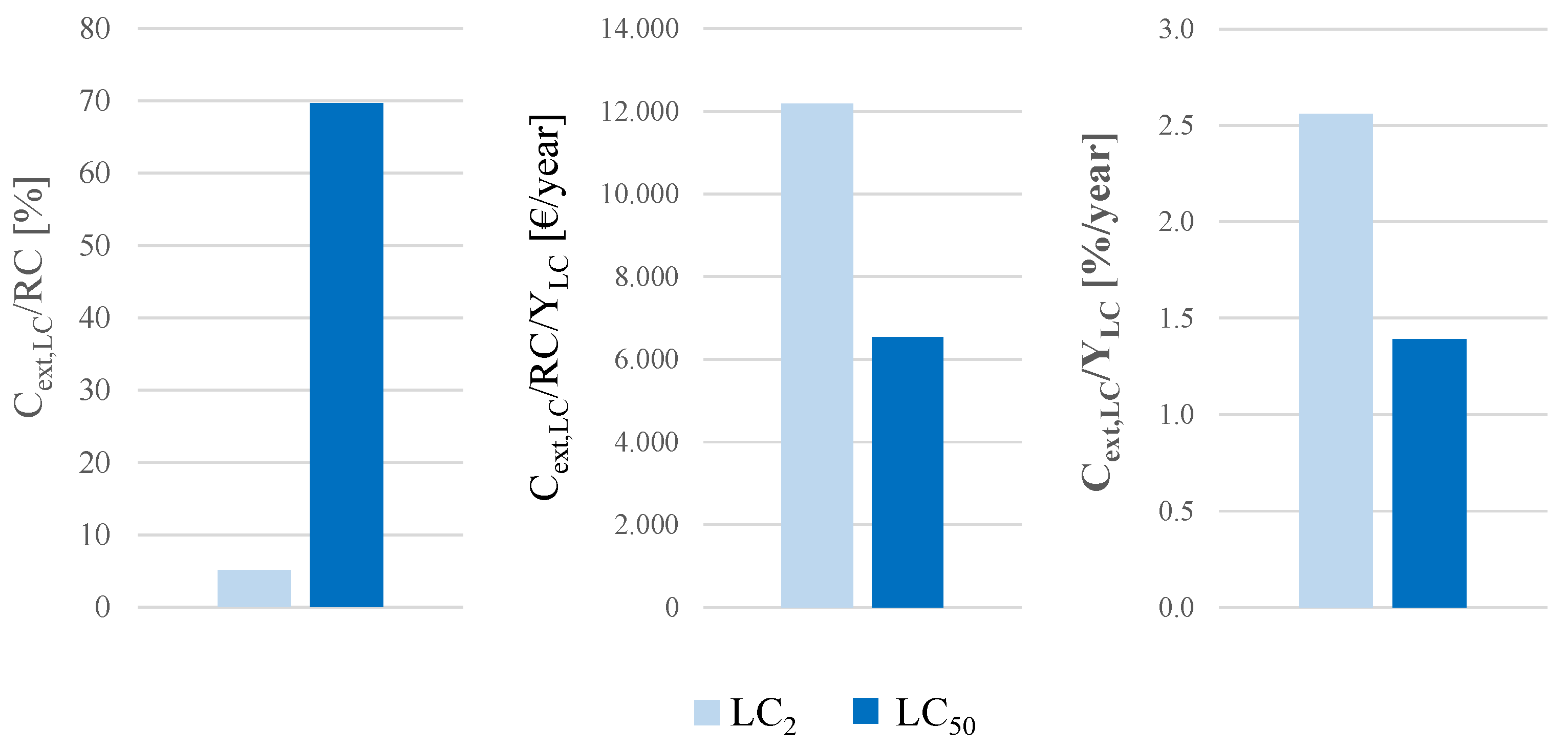
In Figure 11, extraordinary costs ${\mathrm{C}}_{\mathrm{ext},\mathrm{LC}}$ only are expressed as a percentage of the RC, which is indicative of the value of the asset, and in relationship to Y_LC duration. Costs related to the building performance under extraordinary actions are considerable, reaching up to 70% of the RC for Y_LC = 50. On an annual basis, such costs do not exceed 3% of the RC; even though such a share may not seem significant, it becomes considerable if not considered in business-as-usual economic evaluations. ${\mathrm{C}}_{\mathrm{ext},\mathrm{LC}}$ grows spanning from Y_LC = 2 to Y_LC = 50. On the contrary, corresponding annual costs decrease, as a shorter Y_LC does not allow amortization of expenses, and, on the other side, it does not guarantee that the building would not be subject to hazardous events.

4.2. Environmental Impacts

Total ordinary environmental impacts ${\mathrm{E}}_{\mathrm{ord},\mathrm{LC}}$ are calculated as 264,499 kgCO₂e, with ${\mathrm{E}}_{\mathrm{ord},\mathrm{e}}$ contributing as a saving due to the benefits gained from recycling and recovery operations.

Total extraordinary environmental impacts ${\mathrm{E}}_{\mathrm{ext},\mathrm{LC}}$ for LC₂ and LC₅₀ are calculated as 262.0 kgCO₂e and 4951.7 kgCO₂e, respectively, counting for both seismic and flood hazard-related environmental impacts (${\mathrm{E}}_{\mathrm{ext},\mathrm{LC},\mathrm{s}}$ and ${\mathrm{E}}_{\mathrm{ext},\mathrm{LC},\mathrm{f}}$), respectively.

Results are expressed as absolute values in Figure 12 in the two LC scenarios and disaggregated along phases.

Overall results show that ordinary environmental impacts ${\mathrm{E}}_{\mathrm{ord},\mathrm{LC}}$ are the most relevant ones and, among them, construction impacts are strongly prevalent.${\mathrm{E}}_{\mathrm{ord},\mathrm{LC}}$ and ${\mathrm{E}}_{\mathrm{ext},\mathrm{LC}}$ are not comparable, the extraordinary impacts ${\mathrm{E}}_{\mathrm{ext},\mathrm{LC}}$ being only 1.8% of the total costs of E_LC. In terms of environmental impacts, the role of extraordinary events is thus almost negligible. The results obtained for ${\mathrm{E}}_{\mathrm{ext},\mathrm{LC},\mathrm{s}}$ are in line with existing data for a steel building [13]. No other similar study has been found with respect to flood-induced environmental impacts.

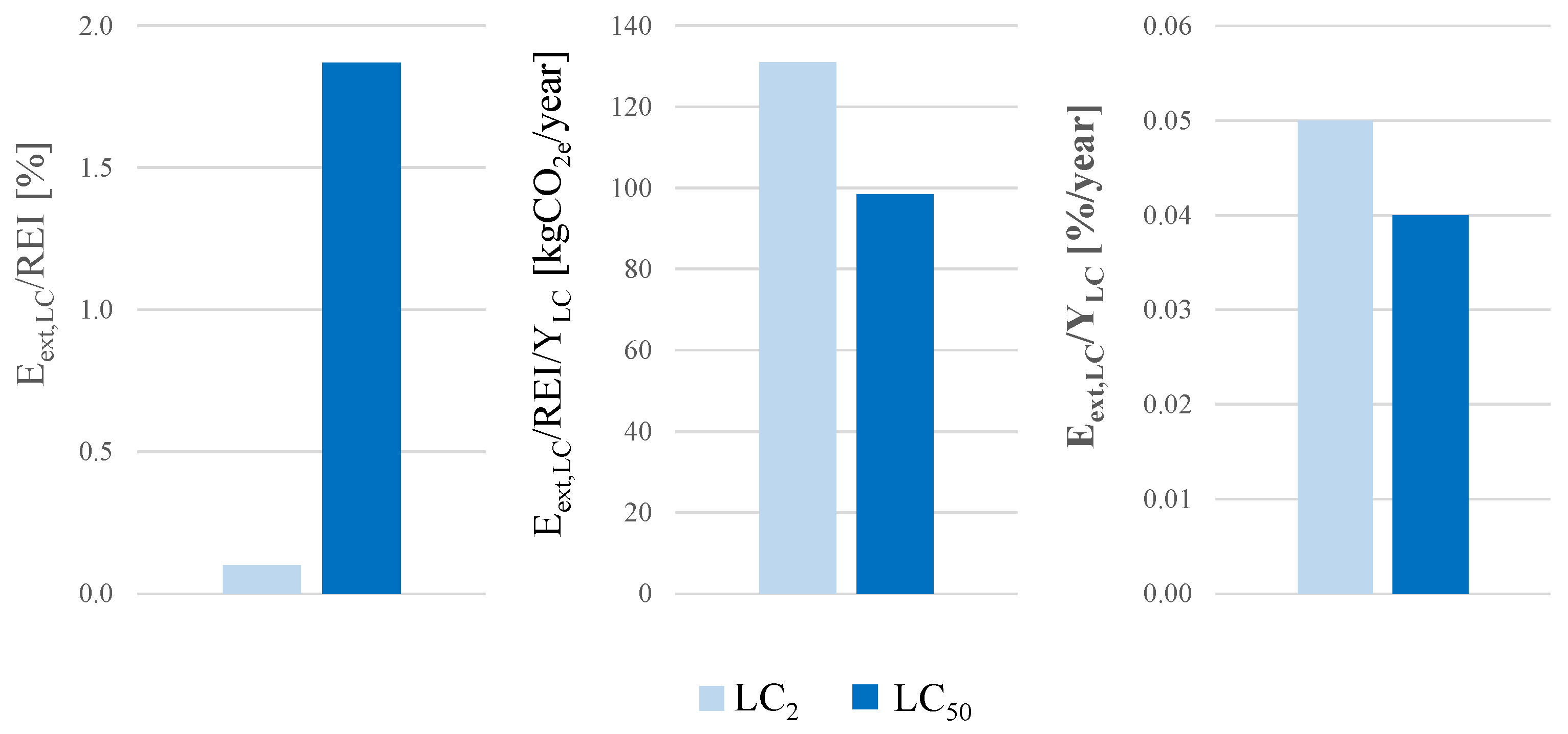
In Figure 13, ${\mathrm{E}}_{\mathrm{ext},\mathrm{LC}}$ is considered as a percentage of the REI, which is indicative of the initial environmental impact of the building, and in relationship to Y_LC duration. The normalized graphs confirm that the relative ${\mathrm{E}}_{\mathrm{ext},\mathrm{LC}}$ is low and does not exceed 0.05% of the REI. Indeed, damage patterns along LC are dominated by non-severe damage states, which under proposed assumptions, do not require elements substitution and thus do not generate environmental impacts (while they are responsible for most economic losses). In addition, steel recycling is highly beneficial in environmental terms, and it allows for the limiting of stresses on the environment.

5. Discussion on Data Availability

The methodology proposed results from several different analyses (e.g., on structures, materials, costs, environmental impacts, etc.), limiting the possibility of ensuring the implementation of a homogenous and coherent approach. Furthermore, analyses require a wide and sector-specific background of information and data (e.g., hazard analysis, damage analysis, structural modeling, cost analysis, etc.). As a result, notable limitations are caused by the lack of available and representative input, and it is recognized that at the present time, the possibility of relying on the proposed comprehensive methodology for building performance evaluation is strongly undermined by the need to introduce multiple proxies and assumptions.

A lack of research background and data is evident, especially for the following topics:

-

Definition of damage states for steel elements, in the function of physical parameters (strain, curvature, etc.);

-

Fragility functions defined within the European context for structural and non-structural components;

-

Characterization of flood hazard in Europe;

-

Structural and non-structural damage evaluation due to flood events, including the absence of fragility functions at the element level.

In addition, inhomogeneity among the level of detail of available data is encountered. For example, seismic hazard is extensively characterized in Italy. However, the availability of fragility functions for structural components designed according to Italian or European specifications is rare, resulting in difficulties in seismic damage evaluation.

6. Conclusions

In this study, a procedure for the analysis of the economic and environmental performance of structures in their life cycle, including not only ordinary costs along life cycle phases but also the extraordinary costs resulting from damage and anticipated end-of-life caused by unexpected natural hazards, is outlined. Its reliability and applicability are investigated by applying it to a one-story steel office building as a case study. Two life scenarios, having a duration of 2 years and 50 years, respectively, and two hazards, namely earthquake, and flood are considered in the analysis.

The results of the case study show that both from an economic and environmental perspective, it is important to consider the entire life cycle of the building in order to produce reliable and representative information to guide the decision-making process.

From an economic perspective, results show that initial costs represent the most significant costs (being almost 60% of the overall costs C_LC if an LC scenario of 50 years is considered), but losses related to natural hazards also represent a relevant contribution to the overall expected cost (up to 40% of the overall cost C_LC if an LC scenario of 50 years is considered), being even predominant over the costs of the end-of-life management. Among extraordinary costs, those related to seismic events are prevalent ${\mathrm{C}}_{\mathrm{ext},\mathrm{LC},\mathrm{s}}$ being 29% of the overall costs C_LC for Y_LC = 50 (against 12% related to floods).

From an environmental perspective, it arises that the most significant environmental results are related to the assessment of ordinary impacts, including end-of-life scenarios, whilst losses due to natural hazard appear to be negligible for the selected case study. In fact, extraordinary environmental impacts ${\mathrm{E}}_{\mathrm{ext},\mathrm{LC}}$ are only 1.8% of the total impacts E_LC. The main reason for these results is that damage patterns along LC are dominated by non-severe damage states, which under proposed assumptions, do not require elements substitution and thus do not generate environmental impacts (while they are responsible for most economic losses).

Thus, it appears that to pave the way to an integrated design approach—to optimize as many performances as possible over the life-cycle—the current design approach is not sufficiently advanced, and it should be accompanied by more refined and specific analyses and by a larger quantity of outputs.

Nevertheless, limitations preventing the use of comprehensive methodologies such as the one proposed in this study still exist. Additionally, implementing complex methodologies considerably complicates the initial phase of the project, as the number of input and output data increases and the pursued objectives are multiple, and the priorities of stakeholders and investors are often focused on money-saving in the short-term scenarios.

However, if these considerations are properly carried out, the benefits in the long term may be significant and valuable, mainly because the choices related to the first phases of the design strongly shape the system’s performance over the whole life.

Future progress is desirable from a double perspective. On the one hand, the procedure of analysis should become more consolidated and more supported by research background and data. On the other hand, sensibility to the issues presented should increase among all the actors involved in a structure design and management.