High-Resolution Hazard Assessment for Tropical Cyclone-Induced Wind and Precipitation: An Analytical Framework and Application

Abstract

Intensified tropical cyclones (TCs) threaten the socioeconomic development of coastal cities. The coupling of strong wind and precipitation with the TC process usually amplifies the destructive effects of storms. Currently, an integrated analytical framework for TC hazard assessment at the city level that combines the joint statistical characteristics of multiple TC-induced hazards and local environmental features does not exist. In this study, we developed a novel hazard assessment framework with a high spatiotemporal resolution that includes a fine-tuned K-means algorithm for clustering TC tracks and a Copula model to depict the wind–precipitation joint probability distribution of different TC categories. High-resolution wind and precipitation data were used to conduct an empirical study in Shenzhen, a coastal megacity in Guangdong Province, China. The results show that the probabilities of TC-induced wind speed and precipitation exhibit significant spatial heterogeneity in Shenzhen, which can be explained by the characteristics of TC tracks and terrain environment factors. In general, the hazard intensity of TCs landing from the west side is higher than that from the east side, and the greatest TC intensity appears on the southeast coast of Shenzhen, implying that more disaster prevention efforts are needed. The proposed TC hazard assessment method provides a solid base for highly precise risk assessment at the city level.

1. Introduction

This past decade has been marked by devastating extreme events, including Hurricane Harvey in 2017, Typhoon Lekima in 2019, and Typhoon Rai in 2021. Climate change has intensified tropical cyclones (TCs), posing a greater threat to life and property along coastal areas [1,2]. With the influence of the anthropogenic rise in greenhouse gases, cyclone track density, power dissipation, and cyclone genesis have shown robust increasing trends over the North Pacific [3,4]. In addition, the development of infrastructure in coastal areas, especially in developing countries, has accelerated. As a result, risks have increased with the urban infrastructures from more severe TCs [5]. TC hazard assessment at a high spatial resolution is an inevitable and fundamental step for risk assessment.

The demand from stakeholders for information on natural hazards has been highlighted in several reports, such as Global Assessment Reports on Disaster Risk Reduction and IPCC SREX. Comprehensive hazard assessment is essential to achieving the Millennium Development Goals, Sustainable Development Goals, and the Sendai framework. Knowledge of natural hazards is key to developing preventative policies and taking risk-reduction measures. Such information is valuable to stakeholders from the (re)insurance, governance, and spatial planning sectors.

Many empirical models consider that TC hazards vary among different areas, provinces, cities, and even greater regions. However, the spatial or temporal resolution of previous studies has generally been rough, making it difficult to illustrate the hazards of a TC process at the city level. How do TC hazards vary within a city? What factors can explain the variation? In contrast to the extensive studies of inventory exposure to TCs with a high spatiotemporal resolution, these questions have not received adequate attention. High-resolution TC hazard assessment is urgently needed for refined risk analysis and emergency management in coastal cities. For a more accurate impact analysis of TCs, hazard assessments with a high temporal resolution are needed to depict the changes during a TC process. Additionally, hazard assessments with a high spatial resolution are also essential to match the heterogeneously distributed urban infrastructures in cities. Meanwhile, a single factor of TC, such as wind speed, cannot fully reflect the compound impacts of TCs, which usually include strong winds, rainfall, and flooding [6]. Therefore, the combined possibilities of the intensity and frequency of multiple hazards caused by TCs should be considered simultaneously. In addition, the location and direction of TCs affect the scope and distribution pattern of wind and rain in coastal cities [7,8], such that the hazards of different TC categories should be assessed separately.

To address the above issues, we developed a hazard assessment framework with a high spatiotemporal resolution to analyze regional TC hazards. In the framework, TC tracks are clustered by a fine-tuned K-means algorithm, and the wind–precipitation joint probability distribution of different TC categories is depicted by a Copula model. The proposed framework focuses on the short-term wind–rain joint occurrence probability during TC processes and enables subsequent fine-grained risk analysis. To the best of our knowledge, this is the first TC hazard assessment study with such a high temporal and spatial resolution. The outcomes can also be used to plan and schedule disaster preparedness and response operations in urban areas.

The paper is organized as follows. Section 2 reviews previous studies. Section 3 describes the proposed methodological framework, and Section 4 presents a hazard assessment application and results for Shenzhen, China. Thereafter, Section 5 and Section 6 present the discussion and conclusions, respectively.

2. Literature Review

This section surveys an extensive set of TC clustering techniques and TC hazard assessment methodologies.

2.1. TC Clustering Techniques

In recent years, many clustering algorithms have been used to categorize TCs based on their features, such as TC tracks, forms, lengths, or intensities, from TC databases, among which tracks (longitudes and latitudes) have been the most widely used. The key for a clustering algorithm is clustering the data into several groups based on some similarity measures such that the total variance among the groups is minimized. The K-means algorithm is a straightforward and widely used partitioning method that seeks to assign each track to one of K groups [9,10,11]. However, difficulties arise because of the differentiated TC evolution processes, which result in very different point shapes and lengths. The typical K-means algorithm is not suitable for TC tracks of different lengths, and we show that this is a serious shortcoming for TCs. Hu et al. interpolated different tracks to obtain the same length of vectors [12], which added errors. Tian et al. detected interdecadal changes in the genesis of TCs in the western North Pacific based on pHash and K-means cluster analysis [13]. Chand et al. [14] and Samuel et al. [15] used the curve-clustering approach to classify TC tracks. Camargo et al. developed a special probabilistic clustering algorithm that relies on a regression mixture model to cluster TC tracks [16,17]. These techniques provide a mixture of polynomial regression functions (curves) to fit the geographical shapes of trajectories. The Hausdorff distance is a simple dissimilarity measure and is widely used for comparing point sets [18] and image identifying [19]. The combination of the K-means algorithm and the Hausdorff distance can be a new way to cluster the irregular point sets.

2.2. TC Hazard Assessment

There are two main categories of TC hazard assessment methodologies. The first category consists of comprehensive index constructions, including the weighting, normalization, and mechanism-based methods. The weighting method gives weights to different hazard factors according to their importance, occurrence probability, or hazard intensity [20]. The normalization method normalizes a variety of indices into a single index, which is convenient for comprehensive probability analysis [21,22]. However, in these methods, the relationship among factors is characterized as linear, while it is nonlinear for actual TCs. Some researchers have constructed comprehensive indices based on the physical mechanisms or economic characteristics of TCs, such as Accumulated Cyclone Energy [23], Integrated Kinetic Energy [24], and Carvill Hurricane Index [25]. These comprehensive indices mainly focus on winds and fail to consider other TC-induced hazards (e.g., precipitation).

The other category consists of joint probability models, which construct a joint probability distribution function based on multi-hazard correlations. The Copula theory uses marginal distributions to form a joint distribution. It can solve nonlinear, nonnormal, nonsymmetric, and long-tailed problems. In recent years, this theory has been widely used in multivariate analysis in the fields of extreme value theory [26], financial risk [27], wireless communication [28], drought [29,30], and flood disasters [31,32]. Some researchers have previously constructed the TC-induced wind–rain joint probability distribution function based on Copula theory. However, the data are mainly the maximum or accumulated value of annual statistics [33] or TC events [6,34] from a single meteorological station. Recent studies have used meteorological data from multiple stations to depict the regional difference of hazard intensity [35,36]. These studies have indicated that Copula theory can be an effective tool for TC hazard assessment.

3. Methodological Framework

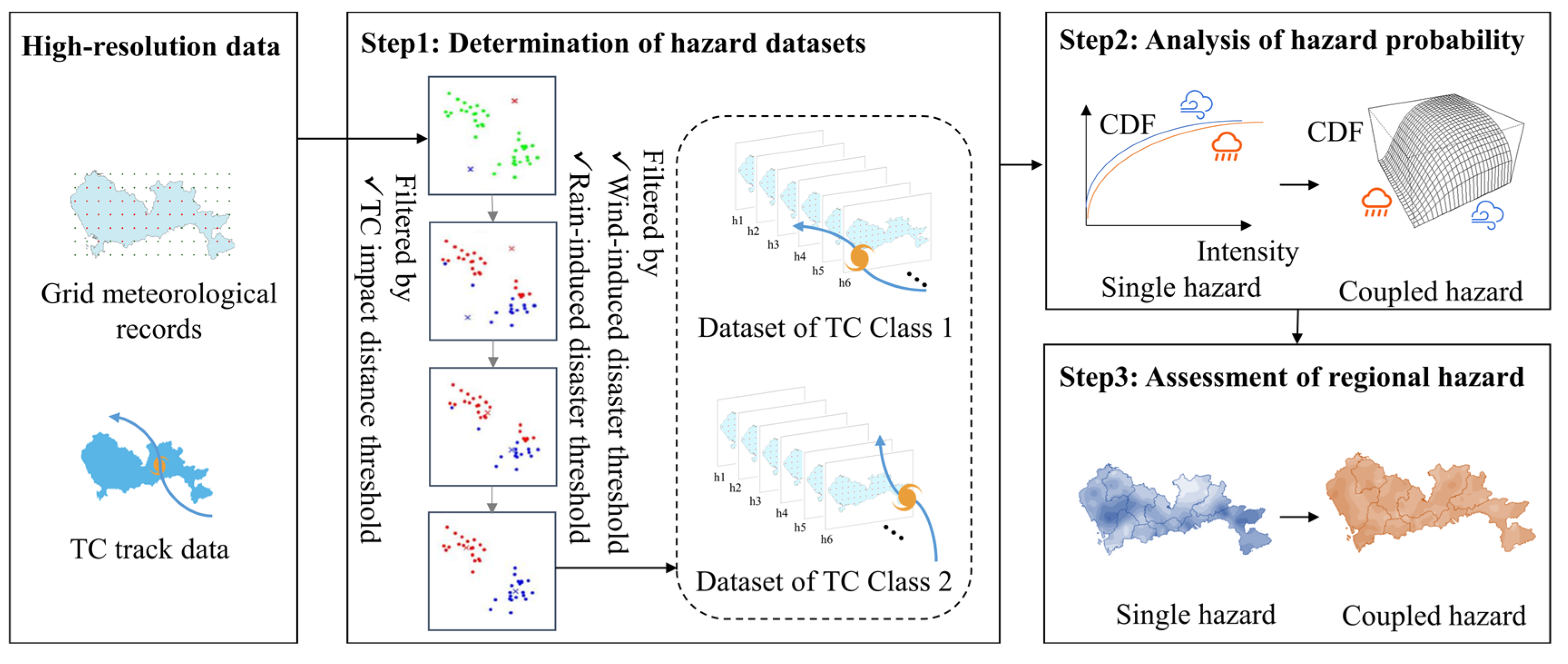
In this paper, a novel TC hazard assessment framework is proposed and divided into three steps: determination of hazard datasets, analysis of hazard probability, and assessment of regional hazards. The analytical framework of this work is shown in Figure 1.

3.1. Hazard Datasets

3.1.1. Disaster Thresholds

The proposed framework assesses wind and rain, the two representative TC-induced hazards. Wind and rain have a significant influence on society, as they commonly lead to storm surges, floods, and debris flows. Our goal is to assess the comprehensive hazard intensity of short-term wind or rain exceeding certain thresholds during TC processes. Therefore, we set the distance threshold from the location to the TC center to determine if the wind and rain are induced by the TC and the intensity thresholds to determine if a hazard of a certain intensity will cause damage.

The thresholds used in this study include the TC impact distance threshold, wind-induced disaster threshold, and rain-induced disaster threshold. (1) TCs in the western Pacific Ocean are nearly circular circulation systems, with a typical radius of approximately 200–500 km [37]. Previous studies have shown that rainfall within 5° in longitude-latitude (approximately 500 km) from the TC center can be considered TC-induced rainfall [38], which is also consistent with on-site evidence. Therefore, we used a circle with a radius of 500 km from the TC center as the TC impact distance threshold. (2) According to the national standard of Grade of tropical cyclones https://www.codeofchina.com/standard/GBT19201-2006.html (accessed on 23 October 2022), a tropical depression is defined when the maximum 2 min mean wind speed near the TC center exceeds 10.8 m/s. Therefore, we set 10.8 m/s as the wind-induced disaster threshold. (3) According to the national standard of Grade of precipitation https://www.codeofchina.com/standard/GBT28592-2012.html (accessed on 23 October 2022), the precipitation was divided into seven levels. In this study, we chose the precipitation reaching the storm level (50 mm/24 h) as the rain-induced disaster threshold.

3.1.2. The Fine-Tuned K-Means Algorithm

In a general K-means algorithm, the data are mapped into points in a Euclidean space and clustered into several classes. These classes can be natural groups of variables, data points, or objects similar to one another in terms of some similarity measures. The clustering performance is evaluated by using the sum of squares for the error from each data point to the clustering center, as shown in Equation (1).

$$S_T={\displaystyle \sum }_{i=1}^K{\displaystyle \sum }_{e_j\in P_i}\Vert e_j-c_i\Vert {}^2$$

(1)

Here, K is the number of classes; $c_i$ is the clustering center of Class i; $P_i$ is the dataset for Class i; $e_j$ is the location attribute of TC track j (the latitudes and longitudes of TC centers); and $\Vert e_j-c_i\Vert$ is the Euclidean distance from $e_j$ to $c_i$.

The iterative calculation process of K-means is as follows:

(1)

Select K TC tracks as the initial clustering center.

(2)

Calculate the Euclidean distances from all the tracks to each clustering center and assign them to the nearest class.

(3)

Calculate the mean value of all data in each class as the new clustering center.

(4)

End if $S_T$ converges or the number of iterations reaches the preset maximum; otherwise, return to Step (2).

K-means cannot accommodate tracks of different lengths [37]. To address this problem, we fine-tuned the distance calculation in the algorithm by changing the Euclidean distance of two points to the Hausdorff distance of two point sets [38]. The Hausdorff distance is defined as follows:

$$H\left(A,B\right)=\max \left[h\left(A,B\right), h\left(B,A\right)\right]$$

(2)

Here,

$$h\left(A,B\right)=\underset{a\in A}{\max } \underset{b\in B}{\min }\Vert a-b\Vert$$

(3)

$$h\left(B,A\right)=\underset{b\in B}{\max } \underset{a\in A}{\min }\Vert b-a\Vert$$

(4)

$H\left(A,B\right)$ is the bidirectional Hausdorff distance between point sets A and B, $h\left(A,B\right)$ is the unidirectional Hausdorff distance from A to B, and correspondingly, $h\left(B,A\right)$ is the Hausdorff distance from B to A. $H\left(A,B\right)$ is larger than $h\left(A,B\right)$ and $h\left(B,A\right)$, which measures the maximum mismatch between two point sets. In this study, the K-means clustering algorithm was reconstructed using the Hausdorff distance.

The fine-tuned K-means algorithm used in this study to fit the geographical shape of the trajectories allows the clustering to be posed and accommodates TC tracks of different lengths. The filtered TC tracks might be composed of the longitudes and latitudes of TC centers with different numbers, that is, have different lengths and shapes. The proposed method is more objective and simpler than the mixture K-means method used in previous studies.

We determined the hazard datasets in three steps. First, we filtered out the historical TC tracks by using the TC impact distance threshold. Second, we split the TC tracks according to the fine-tuned K-means clustering algorithm. Third, we filtered the meteorological data by using the wind-induced disaster threshold and rain-induced disaster threshold. Thus, the subsequent hazard analysis was carried out based on the subsets of wind speed and precipitation during the impact of different TC classes.

3.2. Analysis of Hazard Probability

The hazards for different TC classes were analyzed during two stages: single hazard of wind or rain and coupled hazards of wind–rain. Single hazard analysis constructs the probability density function (PDF), which indicates the probability of a hazard with different intensities. The probability distribution of a single hazard is the basis of multi-hazard joint probability analysis, commonly known as the marginal distribution. Then, the cumulative distribution function (CDF) of coupled hazards can be further generated based on the two-dimensional (2D) Copula functions.

Copulas are a family of functions that construct the joint distribution of two or more random variables with an unidentified dependence among the variables [39,40]. The most widely used Copula functions include two categories: Elliptic Copulas and Archimedean Copulas. Elliptic Copulas mainly include Gaussian Copula and t Copula, which are suitable when the marginal distribution obeys the standard normal distribution or Student’s T distribution. Archimedean Copulas are obtained by constructing different generator functions, including Clayton Copula, Frank Copula, Gumbel Copula, and Joe Copula (

Table 1. Commonly used 2D Archimedean Copulas.

Copulas	$\mathit{C}\left(\mathit{u},\mathit{v};\mathit{\theta }\right)$	Limiting Condition
Clayton Copula	${\left[\max \left\{u^{-\theta }+v^{-\theta }-1;0\right\}\right]}^{-1/\theta }$	$\theta \in \left[-1,\infty \right]$
Frank Copula	$-\frac{1}{\theta }\log \left[1+\frac{\left(\exp \left(-\theta u\right)-1\right)\left(\exp \left(-\theta v\right)-1\right)}{\left(\exp \left(-\theta \right)-1\right)}\right]$	$\theta \ne 0$
Gumbel Copula	$\exp \left[-({(-\log \left(u\right))}^{\theta }+{\left(-\log \left(v\right){)}^{\theta }\right)}^{\frac{1}{\theta }}\right]$	$\theta \in \left[1,\infty \right]$
Joe Copula	$1-{\left({\left(1-u\right)}^{\theta }+{\left(1-v\right)}^{\theta }-{\left(1-u\right)}^{\theta }\ast {\left(1-v\right)}^{\theta }\right)}^{\frac{1}{\theta }}$	$\theta \in \left[1,\infty \right]$

).

Here,$u$ and $v$ are the marginal distributions of two variables, $\theta$ is the Copula function parameter, and $C\left(u,v;\theta \right)$ is the 2D Archimedean Copula.

We constructed a multi-hazard joint probability model based on 2D Copula theory, which was divided into the following four steps:

(1)

Determine the marginal distribution of the wind speed and precipitation;

(2)

Measure the correlation among the hazards;

(3)

Estimate the parameters of Copula functions that may be applicable;

(4)

Select the appropriate Copula function to fit the joint distribution. Then, the probability of multiple hazards with different intensities can be calculated.

To choose the marginal distribution and joint distribution in Steps (1) and (4), we first determined if the variable was subject to the fitted distribution type based on the Kolmogorov-Smirnov (K-S) test. Then, we selected the best fitting function based on the Akaike information criterion (AIC) minimum, Bayesian information criteria (BIC) minimum, and log-likelihood (LogLik) maximum principle. The calculation formulas are shown in Equations (5)–(8).

$$AIC=2k-2\ln \left(L\left(\theta \right)\right)$$

(5)

$$BIC=kln\left(n\right)-2\ln \left(L\left(\theta \right)\right)$$

(6)

$$L\left(\theta \right)={{\displaystyle \prod }}_{i=1}^{m}p\left(y_i;\theta \right)$$

(7)

$$LogLik\left(\theta \right)=lnL\left(\theta \right)$$

(8)

where $y_i$ is the data sample, and $p\left(y_i;\theta \right)$ is the PDF of the fitting function.

According to the single-hazard $X$ occurrence probability $P_{\left(x\right)}=P\left(X\ge x\right)=1-F\left(x\right)$, we defined two kinds of double-hazard joint occurrence probability. $P_{{\displaystyle \cup }\left(x_1,x_2\right)}$ indicates the probability of at least one hazard reaching a specific intensity, while $P_{{\displaystyle \cap }\left(x_1,x_2\right)}$ indicates the probability of two hazards reaching a specific intensity simultaneously. The calculation formulas are shown in Equations (9) and (10).

$$P_{{\displaystyle \cup }\left(x_1,x_2\right)}=P\left(X_1\ge x_{1}or{X}_2\ge x_2\right)=1-F\left(x_1,x_2\right)$$

(9)

$$P_{{\displaystyle \cap }\left(x_1,x_2\right)}=P\left(X_1\ge x_1 and{X}_2\ge x_2\right)=1-F_{X_1}\left(x_1\right)-F_{X_2}\left(x_2\right)+F\left(x_1,x_2\right)$$

(10)

where $X_1,X_2$ are random variables, their respective CDFs are $F_{X_1}\left(x_1\right) \mathrm{and}{F}_{X_2}\left(x_2\right)$, and the joint CDF of the Copula function is $F\left(x_1,x_2\right)$.

In this study, we fitted the marginal distributions of the hourly wind and precipitation data separately and then fitted the joint distribution of the coupled wind and precipitation by Copula theory. Based on the single or coupled hazard fitting results of different subareas, we quantitatively depicted the characteristics of regional hazards.

4. Application and Results

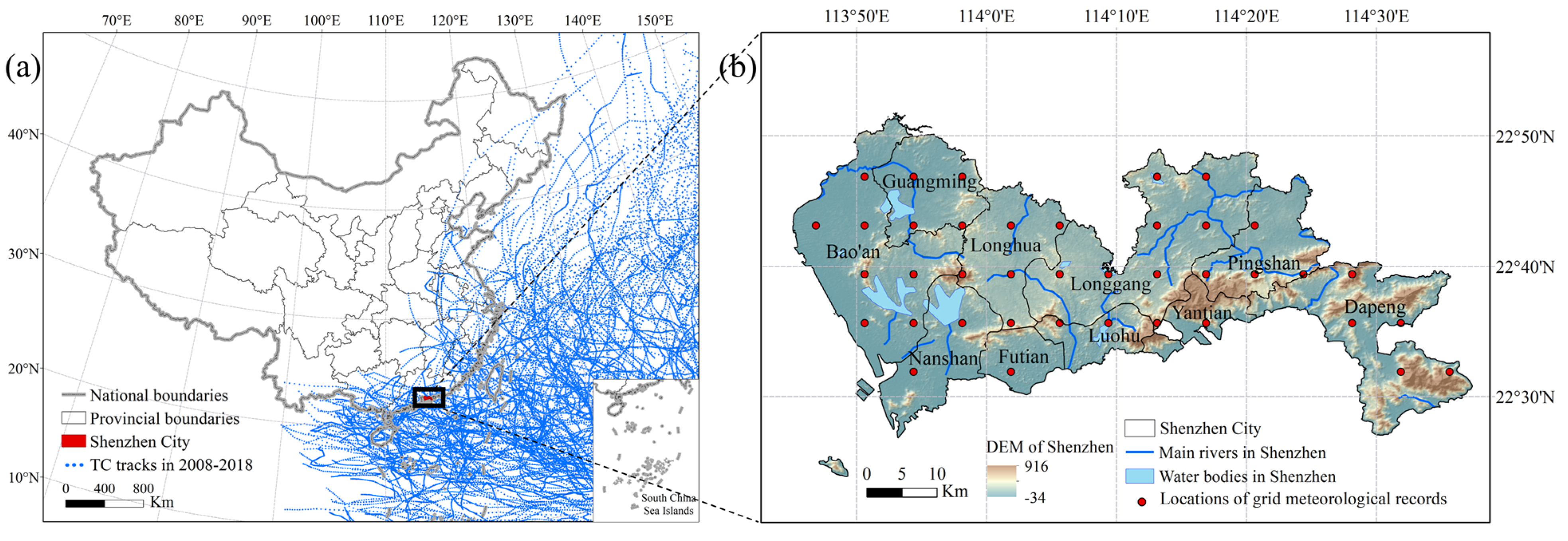
4.1. Study Area and Data Source

Shenzhen, which is an economically developed and densely populated coastal megacity in China, has an area of 1997.47 ${\mathrm{km}}^2$, a GDP of 2.69 trillion yuan and a permanent population of 13.44 million as of 2019 http://www.sz.gov.cn/en_szgov/aboutsz/profile/content/post_10093130.html (accessed on 23 October 2022), a total road mileage of 8066.1 km, and a civilian car ownership of 3.53 million as of 2020 http://tjnj.gdstats.gov.cn:8080/tjnj/2021/directory/15/html/15-11-0.htm (accessed on 23 October 2022). Shenzhen faces the South China Sea and the Pearl River. It has a subtropical oceanic climate. During summer, Shenzhen is vulnerable to frequent TCs from the western Pacific Ocean. With the development of infrastructure, the TC risk to Shenzhen’s transportation system, communication system, and buildings has increased.

Four categories of data were used in this study: (1) the meteorological data of Shenzhen provided by the National Climate Center (NCC), including 10 m wind speed and precipitation data between 1 January 2008 and 31 December 2018 in 39 grid points with resolutions of 0.0625° × 0.0625° and 1 h, respectively http://data.cma.cn/en/?r=data/detail&dataCode=NAFP_CLDAS2.0_NRT (accessed on 23 October 2022); (2) the TC track dataset provided by the NCC, which includes the hourly historical TCs that landed in China from 2008 to 2018. Each record includes the TC ID, year, month, day, time, longitude, and latitude of the TC centers https://tcdata.typhoon.org.cn/en/zjljsjj_sm.html (accessed on 23 October 2022); (3) the 90 m digital elevation model (DEM) of Shenzhen from the NASA SRTM3 dataset https://www.gscloud.cn/ (accessed on 23 October 2022); and (4) the data of the main rivers and water bodies in Shenzhen from the Resource and Environment Science and Data Center https://www.resdc.cn/DOI/DOI.aspx?DOIID=44 (accessed on 23 October 2022). The meteorological data and TC tracks were used to determine the hazard datasets, and the distribution of the DEM and river/water bodies served as a reference for subsequent causative analysis. Figure 2 shows the geographical location of Shenzhen and the distribution of multisource meteorological environment data.

Compared with the annual or TC events in previous studies, the temporal resolution of the hourly data used in this study is considerably enhanced. In meteorological research, one hour is typically acknowledged as a high-precision time unit. When compared to historical weather station observational data utilized for regional hazard studies, the spatial resolution of 0.0625° is significantly more accurate.

4.2. Preprocessing of Hazard Datasets

We filtered out the datasets according to the proposed K-means-based TC track clustering algorithm and three thresholds referred to in Step 1 in Figure 1.

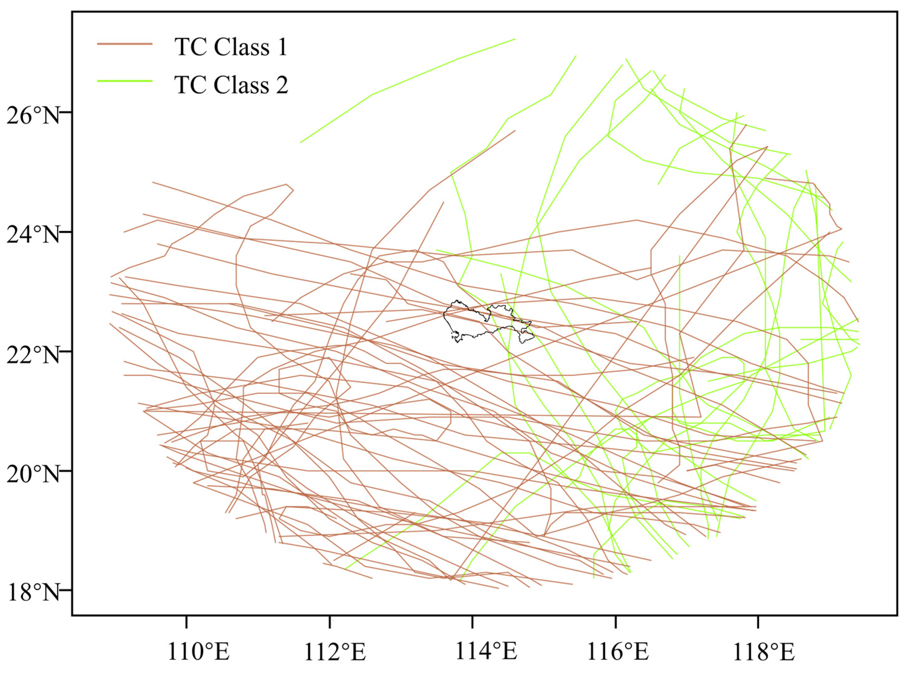
First, for each grid point in Shenzhen, we calculated the distance $d$ from the TC center in all the track records (Figure 2a) to the grid. The grid point was classified as being impacted by TCs at that moment if $d$ ≤ 500 km. From 2008–2018, 74 TCs affected Shenzhen, with an average duration of 47.89 h. Then, we clustered the TC tracks affecting Shenzhen based on the fine-tuned K-means algorithm. We clustered the TC tracks into two classes, and the maximum number of iterations was 100. Figure 3 shows that the two TC classes can be roughly interpreted as landing from the west side of Shenzhen (Class 1) or the east side (Class 2). Furthermore, we retrieved the hourly wind speed and precipitation data for a grid point if the 24 h cumulative precipitation was greater than 50 mm or the wind speed was greater than 10.8 m/s. Thus, we created TC-induced wind speed and precipitation datasets for 39 grid points and 2 TC classes. Approximately 80–200 samples were recorded per grid point for each TC class. Next, we analyzed the TC hazards from the single variable (wind or precipitation) and coupled variables (joint wind–precipitation).

4.3. Hazard Analysis

In this section, we conducted the analysis of hazard probability referred to Step 2 in Figure 1. First, we found a fit for the CDF of observed wind and precipitation data. Then, we specified the Copula method to fit the joint PDFs and CDFs. Later, we appraised the performance of the hazard assessment.

4.3.1. Single Hazard Analysis

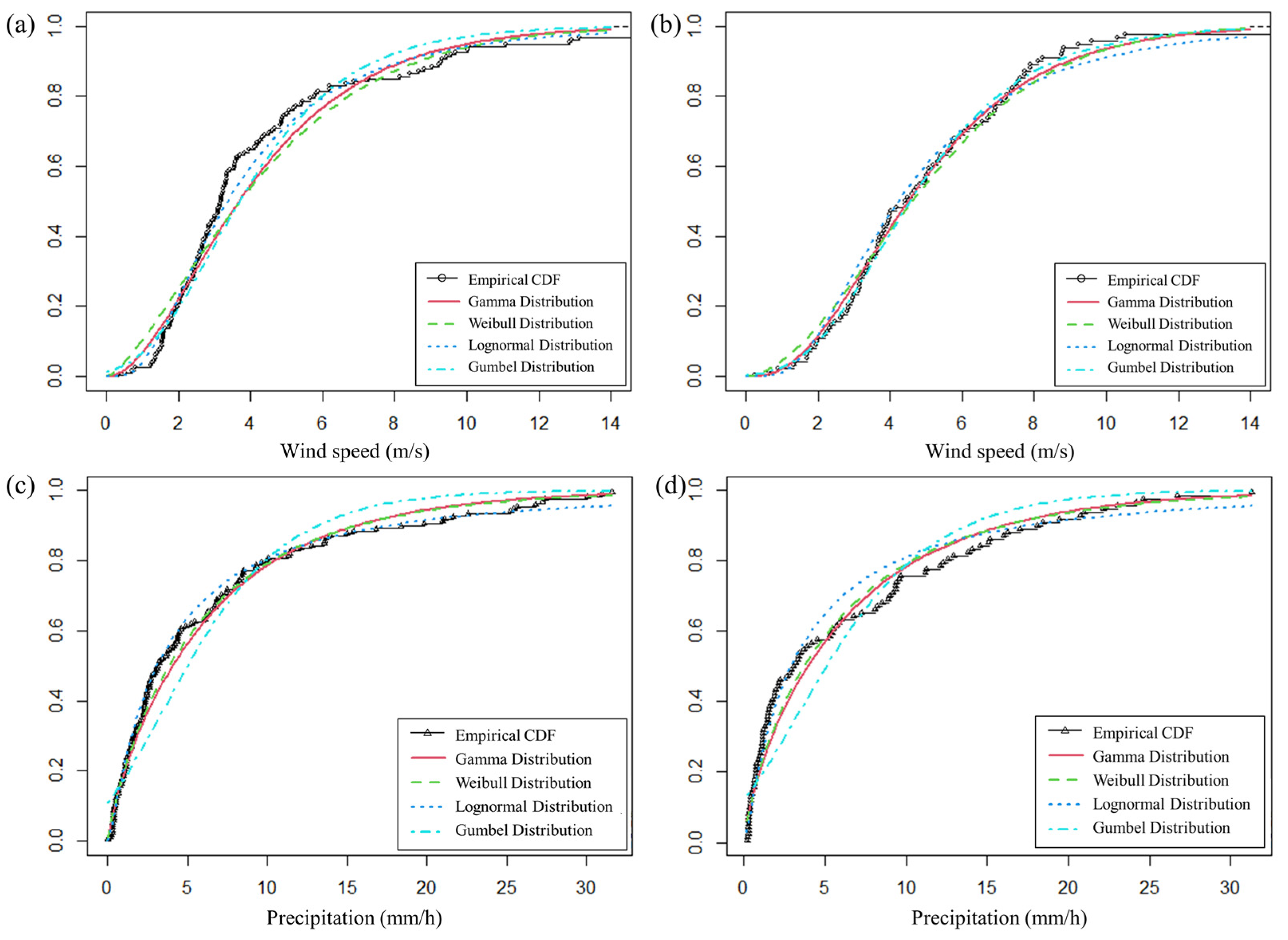
We randomly picked one grid point (denoted by $\mathcal{A}$) as an example to analyze a single hazard. There were 105 records of grid point $\mathcal{A}$ for TC Class 1 and 143 records for TC Class 2. Referring to existing research results [33,34,35], we selected the Gumbel, Weibull, Gamma, and lognormal distributions as the theoretical distribution functions to fit the hourly wind and precipitation data separately. We utilized the maximum likelihood estimate (MLE) approach to estimate the parameters. According to the AIC, BIC, and LogLik values, we found that for two TC classes, Gamma distribution was the best marginal distribution to fit the wind speed data (Figure 4a,b), whereas the lognormal distribution was suitable for fitting the precipitation data (Figure 4c,d).

For TC Class 1, the fitting Gamma CDF $F_1\left(x_1\right)$ of the wind speed data in $\mathcal{A}$ is

$$F_1\left(x_1\right)=\frac{{\displaystyle \int }{0.50}^{2.16}{x}_1{}^{1.16}\exp \left(-0.50x_1\right)}{\mathsf{\Gamma }\left(2.16\right)d{x}_1}$$

(11)

Here, $\mathsf{\Gamma }\left(x\right)={{\displaystyle \int }}_0^{\infty }{t}^{x-1}{e}^{-t}dt$ is the Gamma function with recursion, i.e., $\mathsf{\Gamma }\left(x+1\right)=x\mathsf{\Gamma }\left(x\right)$.

The fitting lognormal CDF $F_2\left(x_2\right)$ of the precipitation in $\mathcal{A}$ is

$$F_2\left(x_2\right)=\frac{1}{2}+\frac{1}{2}erf\left[\frac{\ln \left(x_2\right)-1.13}{1.35\ast \sqrt{2}}\right]$$

(12)

Here, $erf\left(x\right)=\frac{2}{\sqrt{\pi }}{{\displaystyle \int }}_0^x{e}^{-y^2}dy$ is the Gaussian error function.

For TC Class 2, the fitting Gamma CDF $F_1\left(x_1^{\prime }\right)$ of the wind speed data in $\mathcal{A}$ is

$$F_1\left(x_1^{\prime }\right)=\frac{{\displaystyle \int }{0.60}^{3.02}{x}_1^{\prime }{}^{2.02}\exp \left(-0.60x_1^{\prime }\right)}{\mathsf{\Gamma }\left(3.02\right)d{x}_1^{\prime }}$$

(13)

The fitting lognormal CDF $F_2\left(x_2^{\prime }\right)$ of the precipitation in $\mathcal{A}$ is

$$F_2\left(x_2^{\prime }\right)=\frac{1}{2}+\frac{1}{2}erf\left[\frac{\ln \left(x_2^{\prime }\right)-1.07}{1.40\ast \sqrt{2}}\right]$$

(14)

Based on Equations (11)–(14), we calculated the corresponding wind speed and precipitation intensities with different probabilities (

Table 2. The wind speeds and precipitations with different probabilities in $\mathcal{A}$.

TC Classes	Class 1		Class 2
Probability	Wind Speed (m/s)	Precipitation (mm/h)	Wind Speed (m/s)	Precipitation (mm/h)
50%	3.67	3.11	4.50	2.92
20%	6.41	9.72	7.18	9.48
10%	8.25	17.64	8.93	17.57
5%	10.00	28.86	10.56	29.23
1%	13.87	72.64	14.08	75.95
0.5%	15.48	101.84	15.53	107.73

) and the probabilities of different wind speeds (

Table 3. The probabilities of different wind speeds in $\mathcal{A}$.

Grade of TCs	Wind Speed (m/s)	Wind Scale	Probability (Class 1)	Probability (Class 2)
Tropical depression	10.8–17.1	6–7	0.036	0.045
Tropical storm	17.2–24.4	8–9	0.002	0.002
Severe tropical storm	24.5–32.6	10–11	/	/
Typhoon	32.7–41.4	12–13	/	/
Strong typhoon	41.5–50.9	14–15	/	/
Super typhoon	≥51.0	≥16	/	/

/ indicates that the calculated value is too small, the same below.

) and precipitations (

Table 4. The probabilities of different precipitations in $\mathcal{A}$.

Grade of Precipitation	Precipitation (mm/h)	Probability (Class 1)	Probability (Class 2)
Light rain	≤2.5	-	-
Moderate rain	2.6–8.0	0.564	0.544
Heavy rain	8.1–15.9	0.243	0.236
Torrential rain	16.0–49.9	0.113	0.112
Heavy downpour	50.0–99.9	0.020	0.021
Rainstorm	≥100.0	0.005	0.006

) for the two TC classes.

In addition, we found that the gamma distribution and lognormal distribution are also good fits for the TC-induced wind speed and precipitation in other grid points in Shenzhen.

4.3.2. Coupled Hazard Analysis

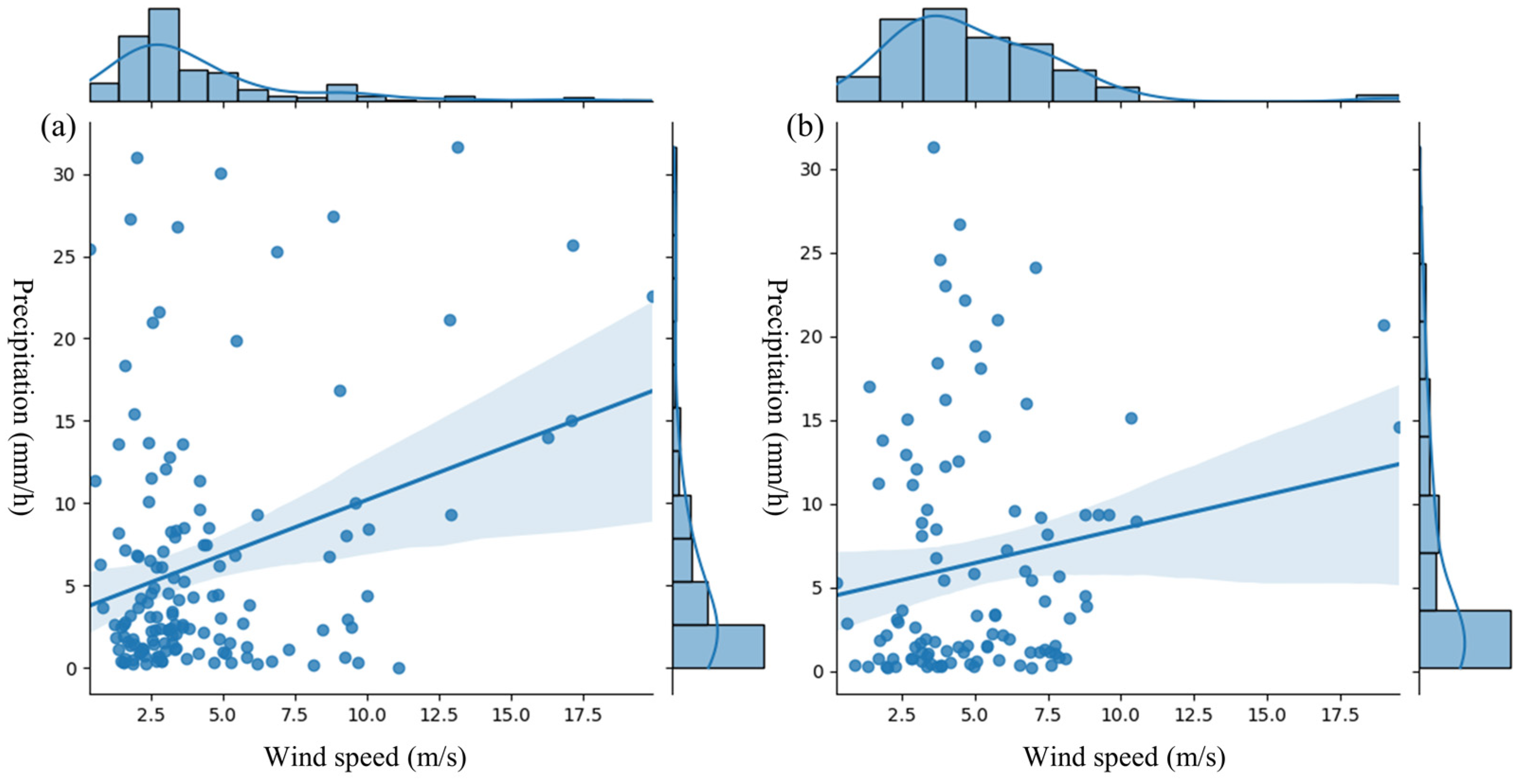
Using grid point $\mathcal{A}$ as an example, the bivariate distribution of hourly wind speed and precipitation is given in Figure 5. The blue line in Figure 5 is the linear regression fit, and the shading along the lines is the confidence interval (95%). There are some points with wind speeds less than 10 m/s and 24 h cumulative precipitation greater than 50 mm. This is consistent with the facts—a typhoon may bring rainfall for several hours, but it is not always windy. At a high temporal resolution, such as one hour, the TC-induced wind and precipitation are not synchronous. The scattered distribution of the wind speed and precipitation in Figure 5 caught our attention. For TC Class 1, the wind–rain correlation was $P_{west}=0.13$, passing the significance test of 0.05. The distributions of the hourly wind and rain data were asymmetric and nonnormal, as indicated by the kurtosis values of the wind speed and precipitation, which were 4.65 and 2.17, and their skewness values, which were 2.07 and 1.71, respectively. For TC Class 2, the wind–rain correlation was $P_{east}=0.17$. The kurtosis values of the wind speed and precipitation were 6.99 and 0.84, and their skewness values were 1.99 and 1.29, respectively. Therefore, we selected Archimedean Copulas to fit the joint probability distribution and estimated the parameters by MLE. We found that the Joe Copula outperformed the other three Copulas in fitting the joint probability of the TC-Class-1-induced wind speed and precipitation in grid point $\mathcal{A}$, but the Clayton Copula performed better for fitting the TC-Class-2-induced wind and precipitation (

Table 5. Comparison of AIC, BIC, LogLik results for Copulas in $\mathcal{A}$.

TC Class	Copulas	$\mathrm{Fitting} \mathit{\theta }$	AIC	BIC	LogLik
Class 1	Clayton	0.32	−6.96	−4.00	4.48
	Frank	0.88	−0.66	2.31	1.33
	Gumbel	1.15	−5.45	−2.48	3.72
	Joe	1.26	−7.85	−4.89	4.92
Class 2	Clayton	0.23	−1.02	−1.63	1.51
	Frank	0.95	−0.64	2.02	1.32
	Gumbel	1.12	−1.00	−1.65	1.50
	Joe	1.18	−0.67	−1.98	1.34

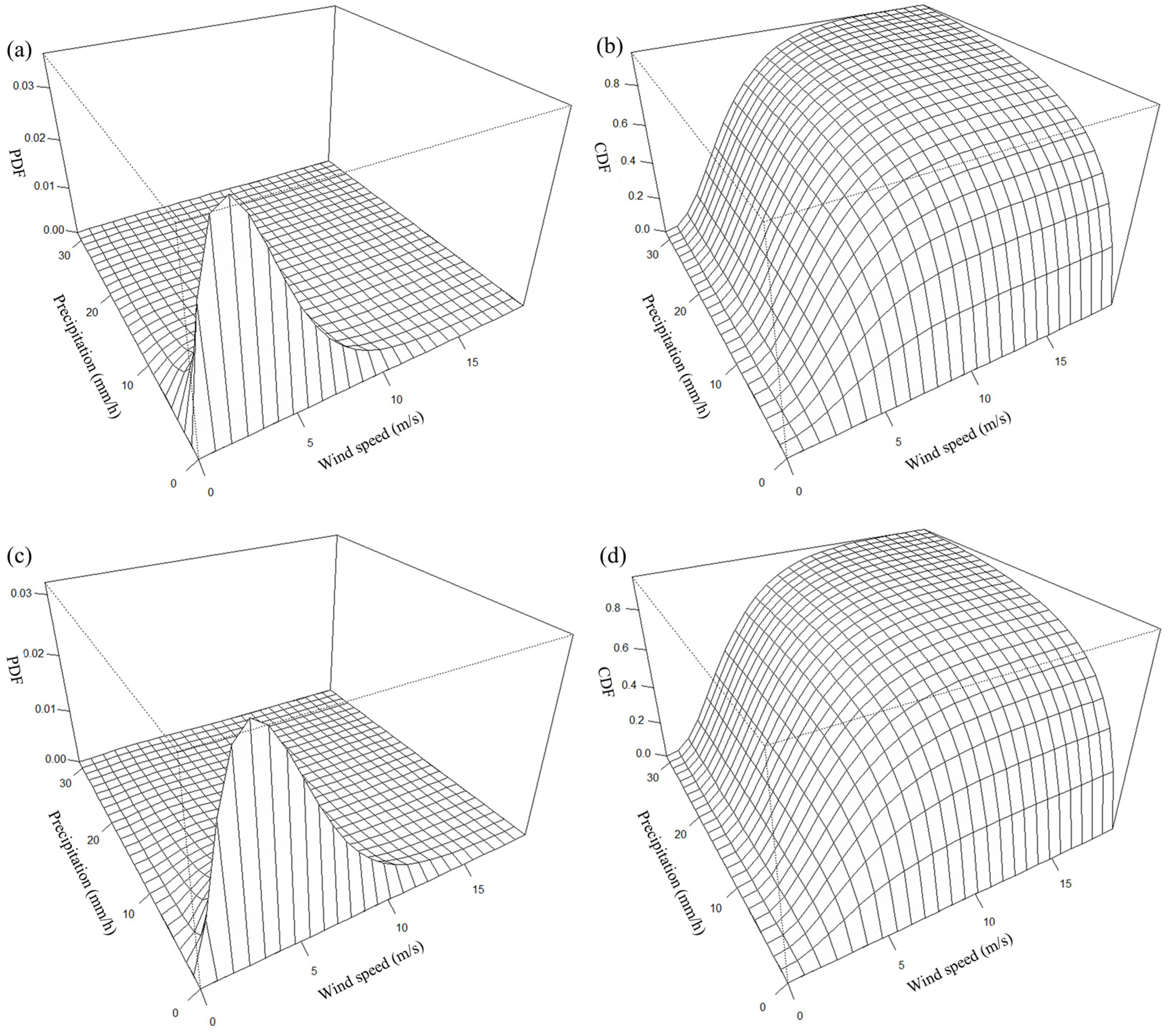
). Figure 6 shows the Copula fitting results in grid point $\mathcal{A}$.

Based on the fitting Copula and marginal distribution of two single hazards, we obtained the joint occurrence probability of double hazards in $\mathcal{A}$. When the TC lands in western Shenzhen (Class 1), the probability of the simultaneous occurrence of a rainstorm and a tropical depression in one hour during the TC process is $P_{{\displaystyle \cap }\left(10.8,16.0\right)}=0.021$, and the probability of occurrence of a rainstorm or tropical depression in one hour is $P_{{\displaystyle \cup }\left(10.8,16.0\right)}=0.136$. When the TC lands on the east side (Class 2), $P_{{\displaystyle \cap }\left(10.8,16.0\right)}=0.017$, $P_{{\displaystyle \cup }\left(10.8,16.0\right)}=0.125$. That is, for grid point $\mathcal{A}$, the TCs landing on the west side of Shenzhen have a higher intensity than those landing on the east side. The results may help prepare for events that have not yet been observed in the past but nonetheless can be expected in the future.

4.3.3. The Performance of Hazard Assessment

Based on the fitting results above, we calculated descriptive statistics, including the mean value, standard deviation (${\mathrm{s}}_d$), coefficient of skewness (${\mathrm{c}}_s$), and their relative error (RE, in %) [41], to demonstrate the performance of the hazard assessment (

Table 6. The comparison of the fitting results in $\mathcal{A}$.

TC Classes	Statistics	Wind Speed					Precipitation
		Single Factor Fitting	Coupled Factor Fitting	Empi-rical Value	RE of Single Factor	RE of Coupled Factor	Single Factor Fitting	Coupled Factor Fitting	Empirical Value	RE of Single Factor	RE of Coupled Factor
Class 1	Mean	4.32	4.31	4.32	0	0	7.72	7.86	6.42	0.20	0.22
	${\mathrm{s}}_{\mathrm{d}}$	2.94	2.96	3.50	−0.16	−0.15	16.86	17.69	7.54	1.24	1.35
	${\mathrm{c}}_{\mathrm{s}}$	1.36	1.49	2.07	−0.34	−0.28	4.84	4.79	1.71	1.83	1.80
Class 2	Mean	5.04	4.25	5.04	0	−0.16	7.75	7.37	6.48	0.20	0.14
	${\mathrm{s}}_{\mathrm{d}}$	2.90	1.35	3.03	−0.04	−0.55	8.35	8.84	7.31	0.14	0.21
	${\mathrm{c}}_{\mathrm{s}}$	2.15	2.93	1.99	0.08	0.47	3.05	2.41	1.29	1.36	0.87

). Here, the descriptive statistics were calculated by Monte Carlo simulation, which consisted of three steps: (1) generating 5000 random numbers obeying the fitted Copula functions, (2) performing a computation of descriptive statistics using the random numbers, and (3) averaging the results across 10 repetitions to eliminate randomness.

Table 6 shows the fitting results of the single and coupled hazards. The descriptive statistics of the single fitting factor were calculated from Equations (11)–(14). The descriptive statistics of the fitting coupled factors were calculated from $C\left(u,v;\theta \right)$ of Joe Copula and Clayton Copula in Table 1; here, $\theta$ is the bold fitting $\theta$ in Table 5, and $u, v$ are taken from Equations (11)–(14). The descriptive statistics of the empirical values were calculated from preprocessed hazard datasets in Section 4.2. Then, we compared the RE of the descriptive statistics between the empirical values and fitting values. Table 6 demonstrates that the hazard assessment performed well because the REs for more than half of the statistics were less than 30%. Comparing the wind speed and precipitation, we found that the fitting REs of the precipitation are larger than those of the wind speed because the wind speed values are mostly concentrated in a smaller range (approximately 0–14 m/s). While the precipitation span is larger (approximately 0–40 mm/h), the extreme precipitation values amplify the bias. Comparing the three statistics, we found that the REs of the mean are small, while the REs of ${\mathrm{s}}_d$ and ${\mathrm{c}}_s$ are large. Because the statistics of the fitting values were generated based on simulation data with randomness, the generated extreme values have a smaller impact on the mean value but a greater impact on ${\mathrm{s}}_d$ and ${\mathrm{c}}_s$.

It should be noted that the uncertainty of the meteorological gridded data, which are interpolated based on the observational data from the weather stations, affects the goodness of the fitting results.

4.4. The Spatial Heterogeneity of TC Hazards

Based on the analysis results of single and coupled hazard probabilities, we further assessed the regional hazards for specific infrastructure risks referred to in Step 3 in Figure 1. Using road traffic as an example, we analyzed the spatial distribution of TC hazards and identified significant heterogeneity. We set the TC disaster threshold for road traffic based on the Technical Specification for Highway Travel Information Service as 10 mm/h for the precipitation and 8 m/s for the wind speed.

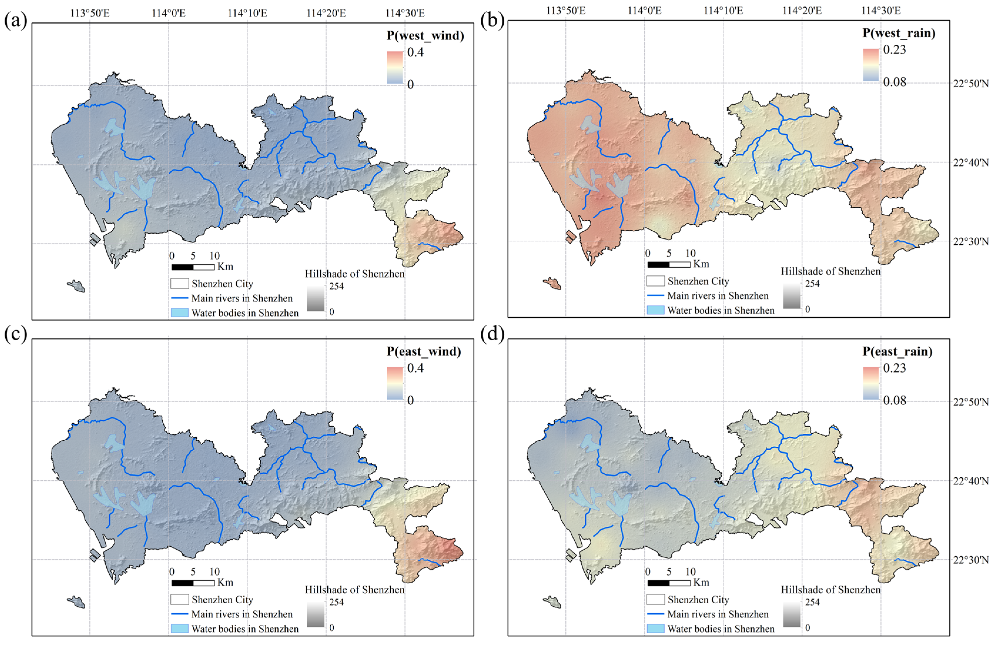
For the 39 grid points in Shenzhen, we used Gamma distribution to fit the wind speed and a lognormal distribution to fit the precipitation for the two TC classes. Then, we calculated the probability of wind speeds over 8 m/s as P(west_wind) and P(east_wind) and the probability of precipitation over 10 mm/h as P(west_rain) and P(east_rain). Figure 7 displays the spatial distribution.

Figure 7a,c demonstrate that the spatial distributions of P(west_wind) and P(east_wind) have a similar pattern regardless of the TC landing location. The east is larger than the west, and the south is larger than the north because the water vapor and surface environment are distinct between the sea and the land, and TCs cause much stronger winds in coastal areas compared to inland areas. In Shenzhen, the TC-induced winds in the west have been significantly weakened due to the blockage of the Pearl River estuary and Hong Kong. The eastern region, particularly Dapeng District, lacks natural barriers and is frequently exposed to severe winds.

Most of western Shenzhen and some of eastern Shenzhen have a higher probability of experiencing rainfall over 10 mm/h when a TC arrives from the west (Figure 7b), whereas small areas of eastern Shenzhen experience rainfall exceeding 10 mm/h when a TC arrives from the east (Figure 7d). This higher probability is due to the terrain and TC tracks. Shenzhen is generally in low hilly areas with mild terraces in between, with a high elevation in the southeast and a low elevation in the northwest. When addressing TCs that are landing from the west, Shenzhen’s western plains and rivers promote significant rainfall, which gradually decreases until it hits gentle hills. The southeast mountains would obstruct the flow while facing TCs arriving from the east. As a result, the elevation causes the wind to be weaker and the rainfall to be heavier on the windward sides. Dense air flow lines at the top and sides of the mountains cause the wind to blow faster. As a result, in the area east of Shenzhen, the likelihood of strong winds would decrease, while the likelihood of heavy rain would change from south to north.

In conclusion, there is a significant spatial difference in the probability of a single hazard affecting road traffic. The most widespread effects of TC-induced rainfall occurred when it arrived from the west. The spatial heterogeneity of TC hazards is influenced by multiple factors of the meteorological environment. These findings validate the necessity and illustrate the importance of high-resolution hazard assessments, especially for accurate urban disaster management.

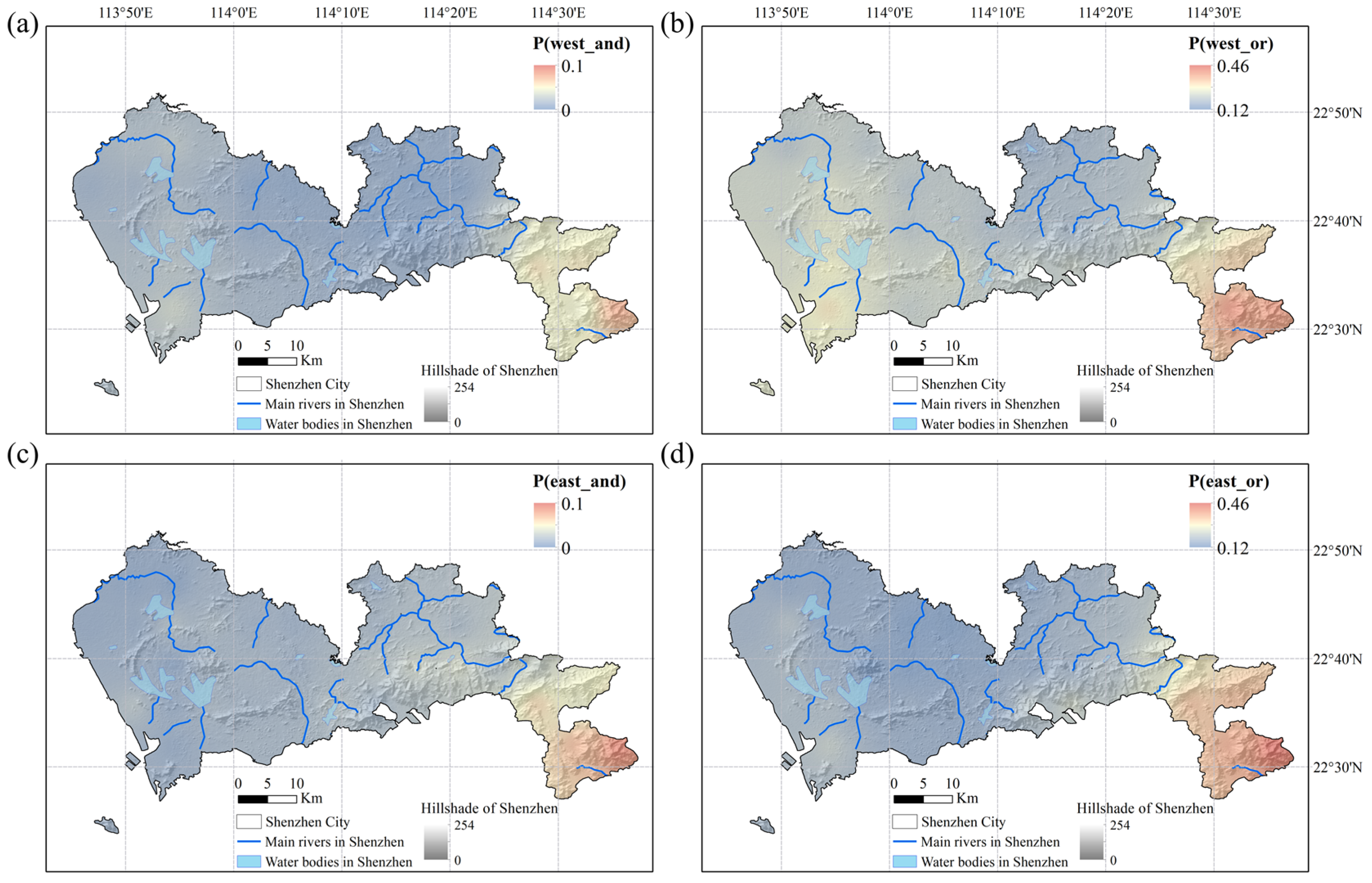
Repeating the calculation process, we tested the fitting performance of Archimedean Copulas for 39 grid points in Shenzhen. Joe Copula and Clayton Copula fit 27 and 12 grid points, respectively, for TCs landing in western Shenzhen (Class 1). For TCs landing in eastern Shenzhen (Class 2), Clayton Copula had a good fitting performance on the combined probability of 28 grid points, and Joe Copula fit well for 11 grid points. Most of the hourly data in our dataset are on the low side, and Clayton Copula is sensitive to changes at the lower tail of the variables. Joe Copula can describe the intense wind and rain because it is more sensitive to changes in the upper tail of the variable. This higher sensitivity indicates that in some areas, a TC-induced rainfall process may be accompanied by extremely high winds and rainfall. We estimated the two double-hazard joint occurrence probabilities for the two TC classes as P(west_and), P(west_or), P(east_and), and P(east_or) based on the best fitted Copula for each grid. The spatial distributions are given in Figure 8.

Dapeng District of Shenzhen is the most vulnerable and in need of catastrophe protection, as indicated in Figure 8. When a TC arrives from the west, the probability of at least one hazard affecting road traffic P(west_or) is approximately 12–46%. Comparing the colors of Figure 8b,d, we find that P(west_or) is larger than P(east_or) in most areas of Shenzhen, especially in western Shenzhen. The analysis results of grid point $\mathcal{A}$ show that the wind–rain hazard of TCs arriving from the west is higher than that of TCs arriving from the east, and this finding is also applicable to the other area in Shenzhen.

5. Discussion

The trend in hazard assessment is toward high resolutions for refined risk analysis and emergency management. Figure 5 shows the weak correlation between the hourly wind speed and precipitation during the impact of TCs—this is surprising, but it also makes sense. A typhoon may bring rainfall for several hours, but it is not always windy. At a high temporal resolution, such as one hour, the TC-induced wind and precipitation are not synchronous. In previous studies, a higher correlation has been found by using maximum or cumulative values based on TC events or annual statistics. This finding suggests that we need to consider the time scale differences of TC hazard assessment. Here, we compared the Pearson correlation coefficients of wind and rain over various time scales. Coefficients were used instead of Copulas because Copula fitting results may vary for different time scales. The Pearson correlation coefficient represents the degree of linear correlation between winds and rains. A larger correlation indicates a larger risk of strong winds and heavy rains. Based on the filtered hourly data reaching three thresholds in Section 4.2, we calculated the maximum wind speed and cumulative precipitation for 39 grid points at four time scales, including the hour, rainfall process, TC event, and year. Here, a rainfall process is a set of continuous records with hourly precipitation data greater than 0. We then obtained their Pearson coefficients.

Figure 9 shows a higher and more dispersed correlation when using the cumulative data (rainfall process, TC event, and year scales) than the hourly data. We speculate that the reason is that the temporal accumulation amplifies the compound hazard severity and local spatial heterogeneity. If we evaluate the TC process hazards based on the overall statistics, the higher correlation between multiple hazards would lead to a higher disaster risk. This finding suggests that we need to pay attention to the time scale of TC hazard analysis. For research on the impact of TCs on urban infrastructures that change rapidly, such as urban road transportation, the evolution of a TC process matters. Hazard analysis with a high temporal resolution can help improve the accuracy of determining how TC processes affect urban infrastructures.

From the hazard assessment results based on the high-resolution TC-induced wind rain data in Shenzhen, we found that the probability of the TC-induced wind speed and precipitation displayed a significant spatial heterogeneity, which can be explained by the TC tracks and terrain environment factors. The findings show that the TC hazard assessment results in different regions are customized. However, the proposed framework can be generalized.

6. Conclusions

This study developed a high-resolution framework to assess the regional hazards of wind and rain. This is a key step toward city-scale risk management and infrastructure resilience analysis during TC processes.

The proposed framework was applied to Shenzhen, China. Based on the hazard assessment results, we identified a significant spatial heterogeneity of TC hazards for urban traffic within the city and addressed the importance of high-resolution hazard assessment in urban disaster management. The southeast coast of Shenzhen is the most likely to be affected by TCs, and disaster prevention efforts should be increased. The hazard of TCs arriving from the west is greater than that of TCs arriving from the east, mostly due to the geographical location and terrain environment.

Our framework has the following three advantages: (1) the framework integrates single hazards and coupled hazards at the city level and is combined with joint statistical characteristics of TC hazards and local environmental features; (2) the fine-tuned K-means clustering algorithm provides a simple method to cluster TC tracks of various shapes and lengths and maintains the characteristics of the original data; and (3) the Copula-based joint probability model provides considerable flexibility for additional multiple hazards and can also be expanded to the joint probability distribution of more dimensions.

There are also certain limitations to this study. When studying joint probability based on Copula theory, we need to select the marginal distribution function and joint probability distribution. The outcomes of the joint probability distribution can vary with different models and fitting methods. Discussing the uncertainty of the results in Copula-based hazard analysis is worthwhile. Several extensions to the methodology are anticipated in our future work. We will analyze historical data based on a larger time scale and more dimensions to improve the fitting performance.

Our study can better reveal the interaction between a TC system and the physical environment of Shenzhen. The expected assessment outputs can be used for informed decision making and as a reference for disaster risk reduction.

References

- Balaguru, K.; Foltz, G.R.; Leung, L.R.; Emanuel, K.A. Global Warming-Induced Upper-Ocean Freshening and the Intensification of Super Typhoons. Nat. Commun. 2016, 7, 13670. [Google Scholar] [CrossRef] [PubMed] [Green Version]
- Sobel, A.H.; Camargo, S.J.; Hall, T.M.; Lee, C.; Tippett, M.K.; Wing, A.A. Human Influence on Tropical Cyclone Intensity. Science 2016, 353, 242–246. [Google Scholar] [CrossRef] [PubMed] [Green Version]
- Ying, M.; Chen, B.; Wu, G. Climate Trends in Tropical Cyclone-Induced Wind and Precipitation over Mainland China. Geophys. Res. Lett. 2011, 38, L01702. [Google Scholar] [CrossRef] [Green Version]
- Zhang, L.; Karnauskas, K.B.; Donnelly, J.P.; Emanuel, K. Response of the North Pacific Tropical Cyclone Climatology to Global Warming: Application of Dynamical Downscaling to CMIP5 Models. J. Clim. 2017, 30, 1233–1243. [Google Scholar] [CrossRef]
- Chavas, D.; Chen, J. Tropical Cyclones Could Last Longer After Landfall in a Warming World. Nature 2020, 587, 200–201. [Google Scholar] [CrossRef]
- Ye, Y.; Fang, W. Estimation of the Compound Hazard Severity of Tropical Cyclones over Coastal China During 1949–2011 with Copula Function. Nat. Hazards 2018, 93, 887–903. [Google Scholar] [CrossRef]
- Kumar, A.; Nanda, K.R.B.; Krishna, K.O.; Dev, N. On the Relationship between Intensity Changes and Rainfall Distribution in Tropical Cyclones over the North Indian Ocean. Int. J. Clim. 2020, 40, 2015–2025. [Google Scholar]
- Yu, Z.; Wang, Y.; Xu, H. Observed Rainfall Asymmetry in Tropical Cyclones Making Landfall over China. J. Appl. Meteorol. Clim. 2015, 54, 117–136. [Google Scholar] [CrossRef]
- Il, C.; Lm, L. Cluster Analysis of Philippine Tropical Cyclone Climatology: Applications to Forecasting. J. Climatol. Weather. Forecast. 2016, 4, 1–17. [Google Scholar]
- Fang, W.; Zhang, H. Zonation and Scaling of Tropical Cyclone Hazards based on Spatial Clustering for Coastal China. Nat. Hazards 2021, 109, 1271–1295. [Google Scholar] [CrossRef]
- Samuel, S.B.; Savin, S.C.; Suzana, J.C.; Kevin, J.T.; Chris, T.; Harvey, Y. Western North Pacific Tropical Cyclone Tracks in CMIP5 Models: Statistical Assessment Using a Model-Independent Detection and Tracking Scheme. J. Clim. 2019, 32, 7191–7208. [Google Scholar]
- Hu, F.; Yang, S.; Russell, G.T. Resilience-Driven Road Network Retrofit Optimization Subject to Tropical Cyclones Induced Roadside Tree Blowdown. Int. J. Disast. Risk Sci. 2021, 12, 72–89. [Google Scholar] [CrossRef]
- Tian, Y.; Zhou, W.; Wong, W.K. Detecting Interdecadal Change in Western North Pacific Tropical Cyclone Genesis Based on Cluster Analysis Using pHash + Kmeans. Front. Earth Sci. 2022, 9, 825835. [Google Scholar] [CrossRef]
- Chand, S.S.; Walsh, K.J.E. The Influence of the Madden–Julian Oscillation on Tropical Cyclone Activity in the Fiji Region. J. Clim. 2010, 23, 868–886. [Google Scholar] [CrossRef]
- Samuel, S.B.; Savin, S.C.; Kevin, J.T.; Andrew, J.D.; Chris, T.; Harvey, Y. Projections of Southern Hemisphere Tropical Cyclone Track Density Using CMIP5 Models. Clim. Dynam. 2019, 52, 6065–6079. [Google Scholar]
- Camargo, S.J.; Robertson, A.W.; Gaffney, S.J.; Smyth, P.; Ghil, M. Cluster Analysis of Typhoon Tracks. Part I: General Properties. J. Clim. 2007, 20, 3635–3653. [Google Scholar] [CrossRef]
- Camargo, S.J.; Robertson, A.W.; Gaffney, S.J.; Smyth, P.; Ghil, M. Cluster Analysis of Typhoon Tracks. Part II: Large-Scale Circulation and ENSO. J. Clim. 2007, 20, 3654–3676. [Google Scholar] [CrossRef]
- Marosevic, T. The Hausdorff distance between some sets of points. Math. Commun. 2018, 23, 247–257. [Google Scholar]
- Sung, S.; Lee, E.; Shin, B. Prevention of mountain disasters and maintenance of residential area through real-time terrain rendering. Sustainability 2021, 13, 2950. [Google Scholar] [CrossRef]
- Kakareko, G.; Jung, S.; Vanli, O.A.; Tecle, A.; Khemici, O.; Khater, M. Hurricane Loss Analysis Based on the Population-Weighted Index. Front. Built Environ. 2017, 3, 46. [Google Scholar] [CrossRef] [Green Version]
- Chen, W.; Lu, Y.; Sun, S.; Duan, Y.; Leckebusch, G.C. Hazard Footprint-Based Normalization of Economic Losses from Tropical Cyclones in China During 1983–2015. Int. J. Disast. Risk Sci. 2018, 9, 195–206. [Google Scholar] [CrossRef] [Green Version]
- Somnath, B.; Balamurugan, G.; Ranit, C.; Rajib, S. Geographic Variation of Resilience to Landslide Hazard: A Household-based Comparative Studies in Kalimpong Hilly Region, India. Int. J. Disast. Risk Reduct. 2020, 46, 101456. [Google Scholar]
- Roca-Flores, E.; Naumis, G.G. Assessing Statistical Hurricane Risks: Nonlinear Regression and Time-Window Analysis of North Atlantic Annual Accumulated Cyclonic Energy Rank Profile. Nat. Hazards 2021, 108, 2455–2465. [Google Scholar] [CrossRef]
- Bass, B.; Irza, J.N.; Proft, J.; Bedient, P.; Dawson, C. Fidelity of the Integrated Kinetic Energy Factor as an Indicator of Storm Surge Impacts. Nat. Hazards 2017, 85, 575–595. [Google Scholar] [CrossRef]
- Giovanni, M. Hurricane Lifespan Modeling through a Semi-Markov Parametric Approach. J. Forecast. 2013, 32, 369–384. [Google Scholar]
- Jan, B. On the Effect of Long-Range Dependence on Extreme Value Copula Estimation with Fixed Marginals. Commun. Stat.-Theory Methods 2016, 45, 5590–5618. [Google Scholar]
- Wang, H.; Yuan, Y.; Li, Y.; Wang, X. Financial Contagion and Contagion Channels in the Forex Market: A New Approach via the Dynamic Mixture Copula-Extreme Value Theory. Econ. Model. 2021, 94, 401–414. [Google Scholar] [CrossRef]
- Farshad, R.G.; Ghosheh, A.H. Copula Function-based Analysis of Outage Probability and Coverage Region for Wireless Multiple Access Communications with Correlated Fading Channels. IET Commun. 2020, 14, 1804–1810. [Google Scholar]
- Yuan, Y.; Bao, A.; Jiang, P.; Hamdi, R.; Termonia, P.; De Maeyer, P.; Guo, H.; Zheng, G.; Yu, T.; Prishchepov, A.V. Probabilistic Assessment of Vegetation Vulnerability to Drought Stress in Central Asia. J. Environ. Manag. 2022, 310, 114504. [Google Scholar] [CrossRef]
- Seo, J.; Won, J.; Choi, J.; Lee, J.; Kim, S. A Copula Model to Identify the Risk of River Water Temperature Stress for Meteorological Drought. J. Environ. Manag. 2022, 311, 114861. [Google Scholar] [CrossRef]
- Jang, J.; Chang, T. Flood Risk Estimation under the Compound Influence of Rainfall and Tide. J. Hydrol. 2022, 606, 127446. [Google Scholar] [CrossRef]
- Klaho, M.H.; Safavi, H.R.; Golmohammadi, M.H.; Alkntar, M. Comparison between Bivariate and Trivariate Flood Frequency Analysis Using the Archimedean Copula Functions, A Case Study of the Karun River in Iran. Nat. Hazards 2022, 112, 1589–1610. [Google Scholar] [CrossRef]
- Dong, S.; Jiao, C.; Tao, S. Joint Return Probability Analysis of Wind Speed and Rainfall Intensity in Typhoon-Affected Sea Area. Nat. Hazards 2017, 86, 1193–1205. [Google Scholar] [CrossRef]
- Um, M.; Joo, K.; Nam, W.; Heo, J. A Comparative Study to Determine the Optimal Copula Model for the Wind Speed and Precipitation of Typhoons. Int. J. Clim. 2017, 37, 2051–2062. [Google Scholar] [CrossRef]
- Ming, X.; Xu, W.; Li, Y.; Du, J.; Liu, B.; Shi, P. Quantitative Multi-Hazard Risk Assessment with Vulnerability Surface and Hazard Joint Return Period. Stoch. Environ. Res. Risk A 2015, 29, 35–44. [Google Scholar] [CrossRef]
- Meng, C.; Xu, W.; Qiao, Y.; Liao, X.; Qin, L. Quantitative Risk Assessment of Population Affected by Tropical Cyclones Through Joint Consideration of Extreme Precipitation and Strong Wind—A Case Study of Hainan Province. Earth’s Future 2021, 9, e2021EF002365. [Google Scholar] [CrossRef]
- Jiang, H.; Zipser, E.J. Contribution of Tropical Cyclones to the Global Precipitation from Eight Seasons of TRMM Data: Regional, Seasonal, and Interannual Variations. J. Clim. 2010, 23, 1526–1543. [Google Scholar] [CrossRef]
- Maiseli, B.J. Hausdorff Distance with Outliers and Noise Resilience Capabilities. SN Comput. Sci. 2021, 2, 358. [Google Scholar] [CrossRef]
- Fernández-Sánchez, J.; Úbeda-Flores, M. Proving Sklar’s Theorem Via Zorn’s Lemma. Int. J. Uncertain. Fuzziness Knowl.-Based Syst. 2018, 26, 81–85. [Google Scholar] [CrossRef]
- Nadaf, T.; Lotfi, T.; Shateyi, S. Revisiting the Copula-Based Trading Method Using the Laplace Marginal Distribution Function. Mathematics 2022, 10, 783. [Google Scholar] [CrossRef]
- Chen, L.; Singh, V.P.; Guo, S.; Zhou, J.; Zhang, J. Copula-based Method for Multisite Monthly and Daily Streamflow Simulation. J. Hydrol. 2015, 528, 369–384. [Google Scholar] [CrossRef]
Figure 1.
The analytical framework.
Figure 2.
Case study area: Shenzhen. (a) The geographical location; (b) The distribution of multisource environmental data.
Figure 3.
Clustering results of TCs affecting Shenzhen.
Figure 4.
The fitting Cumulative Distribution Function of the hourly wind speed (a,b) and precipitation (c,d) in grid point for TC Class 1 (a,c) and Class 2 (b,d).
Figure 5.
Bivariate distribution of wind speed and precipitation in grid point for TC Class 1 (a) and Class 2 (b). The blue line is the linear regression fit, and the shading along the lines is the confidence interval (95%).
Figure 6.
The fitting results of the coupled hazards in (a) Joe Copula PDF for TC Class 1; (b) Joe Copula CDF for TC Class 1; (c) Clayton Copula PDF for TC Class 2; (d) Clayton Copula CDF for TC Class 2.
Figure 7.
Spatial distribution of the probability of a single hazard for road traffic. (a) P(west_wind); (b) P(west_rain); (c) P(east_wind); (d) P(east_rain).
Figure 8.
Spatial distribution of the probability of coupled hazards for road traffic. (a) P(west_and); (b) P(west_or); (c) P(east_and); (d) P(east_or).
Figure 9.
The box plot of wind–rain correlation at different time scales.