Article

Temporal Variation and Spatial Distribution in the Water Environment Helps Explain Seasonal Dynamics of Zooplankton in River-Type Reservoir

1
College of Agricultural Science and Engineering, Hohai University, Nanjing 210098, China
2
Wenzhou Water Resources and Conservancy Bureau, Wenzhou 325000, China
*
Authors to whom correspondence should be addressed.
Sustainability 2022, 14(21), 13719; https://doi.org/10.3390/su142113719
Submission received: 6 September 2022 / Revised: 18 October 2022 / Accepted: 19 October 2022 / Published: 22 October 2022
(This article belongs to the Topic Hydrology and Water Resources in Agriculture and Ecology)

Abstract

:
Integrated assessment of the water environment has become widespread in many rivers, lakes, and reservoirs; however, aquatic organisms in freshwater are often overlooked in this process. Zooplankton, as primary consumers, are sensitive and responsive to changes in the water environment. Water and zooplankton samples were collected on-site at Shanxi Reservoir quarterly to determine 12 water environmental indicators and to quantify the abundance of zooplankton of Cladocera, Copepoda and Rotifera by using the ZooScan zooplankton image-scanning analysis system, combined with OLYMPUS BX51 using machine learning recognition classification. The aim was to explore the relationship between water environmental factors and zooplankton through their spatial and temporal heterogeneity. Through principal component analysis, redundancy analysis and cluster analysis, variations in the factors driving zooplankton population growth in different seasons could be identified. At the same time, different taxa of zooplankton can form clusters with related water environmental factors during the abundant water period in summer and the dry water period in winter. Based on long-term monitoring, zooplankton can be used as a comprehensive indicator for water environment and water ecological health evaluation, as well as providing scientific support for regional water resources deployment and management.

Graphical Abstract

1. Introduction

Water is one of the most important natural resources on which all life depends. The earth’s freshwater resources play an important role in the survival of mankind, the development of society, and contemporary progress that cannot be ignored [1,2]. In recent years, however, increasing population and climate change have caused serious pollution and damage to limited freshwater resources [3,4]. Therefore, many water-poor countries around the world, like China, have adopted the construction of reservoirs to collect, store, and utilize their limited freshwater resources [5]. Freshwater reservoirs not only provide water for drinking, agricultural irrigation, and industrial production for nearby residents, but also prevent flooding by regulating the water level downstream through storage and discharge processes [6], and generating electricity through the drainage process can effectively reduce the production of greenhouse gases in the thermal power generation process [7]. Nevertheless, due to human activities, the water environment of freshwater reservoirs in different regions of the world has deteriorated to different degrees [8], which makes the monitoring of the water environment of freshwater reservoirs and the water environment and ecological restoration of freshwater reservoirs a hot topic of current research [9,10]. As freshwater reservoirs are closely related to human production and life, they have been attracting the attention of scholars worldwide in recent years. For a long time, people have been monitoring the water environment and water ecology of freshwater reservoirs through various water environment indicators to ensure water safety and avoiding the crisis caused by water pollution and water environment degradation [11,12]. With the development of science and technology, more and more intelligent equipment and high-tech research methods are applied to water environment monitoring. Sagan, et al. [13] used the potential of remote sensing and the limitations of spectral indices, bio-optical simulations, machine learning, and cloud computing to monitor inland water quality. Shi, et al. [14] used spectroscopic analysis and ultra-high resolution mass spectrometry to monitor dissolved organic matter in wastewater and drinking water treatment.
In addition to conventional water quality indicators, the inclusion of zooplankton-like ecological indicators is an important reference for the comprehensive consideration of the health of the water environment. Zooplankton is an important part of aquatic ecosystems [15,16]. Zooplankton is mostly in the second trophic level of the food web and is the key intermediate link in the transfer of material and energy from primary producers to higher trophic levels [17]. The ecological niche of zooplankton and its specificity has led many researchers to work on integrating it with water environmental indicators. Sousa, et al. [18] found that water quality changes had a significant effect on zooplankton community structure. Due to the widespread use of zooplankton to monitor water quality in productive life as well as in scientific research, in 2011 scholars called for the inclusion of zooplankton in the ecological quality assessment of lakes according to the European Water Framework Directive (WFD) [19]. With further research, it was found that the changes in zooplankton abundance are not only directly related to water environment indicators, but also respond to some extent to changes in the abundance of phytoplankton such as algae [20,21]. Zooplankton species composition and quantity changes are not only the basic content of water ecological health research but can also accurately reflect the quality of the water ecological environment [22,23]. Its biodiversity index is one of the important evaluation indicators of water ecological environment health [4,24].
With the development of computer and electronic technology, more and more researchers rely on the ZooScan zooplankton image scanning and analysis system for scientific and rapid identification, measurement, and identification of zooplankton in the water body [25,26]. Naito, et al. [27] used ZooScan, Optical Plankton Recorder (OPC), and microscopic study methods to study the sea surface zooplankton respectively, and ZooScan has significant advantages among these three quantitative methods. Wang, et al. [28] studied the spatial variation of the size structure of medium-sized plankton and its relationship with environmental factors with the help of the ZooScan system. Maas, et al. [29] used image-based observation systems in marine ecosystems, and with the help of ZooScan, the ecological zonation of zooplankton can be quantitatively analyzed. Noyon, et al. [30] scanned mesozooplankton samples by ZooScan to get the distribution of medium-sized zooplankton communities on the Agulhas Bank in autumn to predict scale structure and production. Garcia-Herrera, et al. [31] used ZooScan in combination with the web-based platform EcoTaxa 2.0 system to study differences in integrated zooplankton abundance, biovolume, and biomass. In addition, the microscope enables accurate species identification and classification of zooplankton [32].
The present study area was conducted in a mountainous riverine freshwater reservoir located in a subtropical monsoonal zone with a mild climate in southeastern China. The study area is in a typhoon area with many inhabitants, and the water environment and water ecology are affected by the combination of extreme typhoon climate and surface pollution from residential areas [33]. During the rainy season, the initial rainwater is mixed with surface pollutants from residential areas into the reservoir due to the catchment effect of the valley [34]. The typhoon season causes drastic changes in the water environment in the reservoir due to the wind disturbance effect [35]. The study area is the main freshwater water source in southern Zhejiang province, which assumes multiple roles as drinking water, domestic water, and industrial water [36], so it is of great importance to maintain water security, guarantee the sustainability of water resources use, and protect the water environment and water ecological stability of the study area.
In this study, zooplankton was linked to its surroundings based on the most important theory in ecology (ecological niche theory) [37], and the spatial and temporal heterogeneity of typical freshwater zooplankton and common water environmental indicators was used to analyze mountain river-type reservoirs. Zooplankton, as an integral part of freshwater aquatic ecosystems, plays an important role in the monitoring and assessment of the water environment [38]. However, studies of the spatial heterogeneity of freshwater zooplankton communities and their correlation with the water environment often take researchers a great deal of time due to the lack of rapid and accurate plankton statistics [39]. Therefore, a systematic study on the spatial distribution of ecological niches of freshwater zooplankton, with the help of OLYMPUS BX51 and ZooScan, a zooplankton image acquisition and analysis system, and an artificial intelligence recognition and classification system, will help to enhance the dimensions of freshwater water environment monitoring. It can also help to explore the spatial and temporal heterogeneity of zooplankton and water environment, identifying the response mechanism of water environment changes to specific zooplankton, and providing new ideas for the sustainable and healthy operation and maintenance of the same type of freshwater reservoirs.

2. Materials and Methods

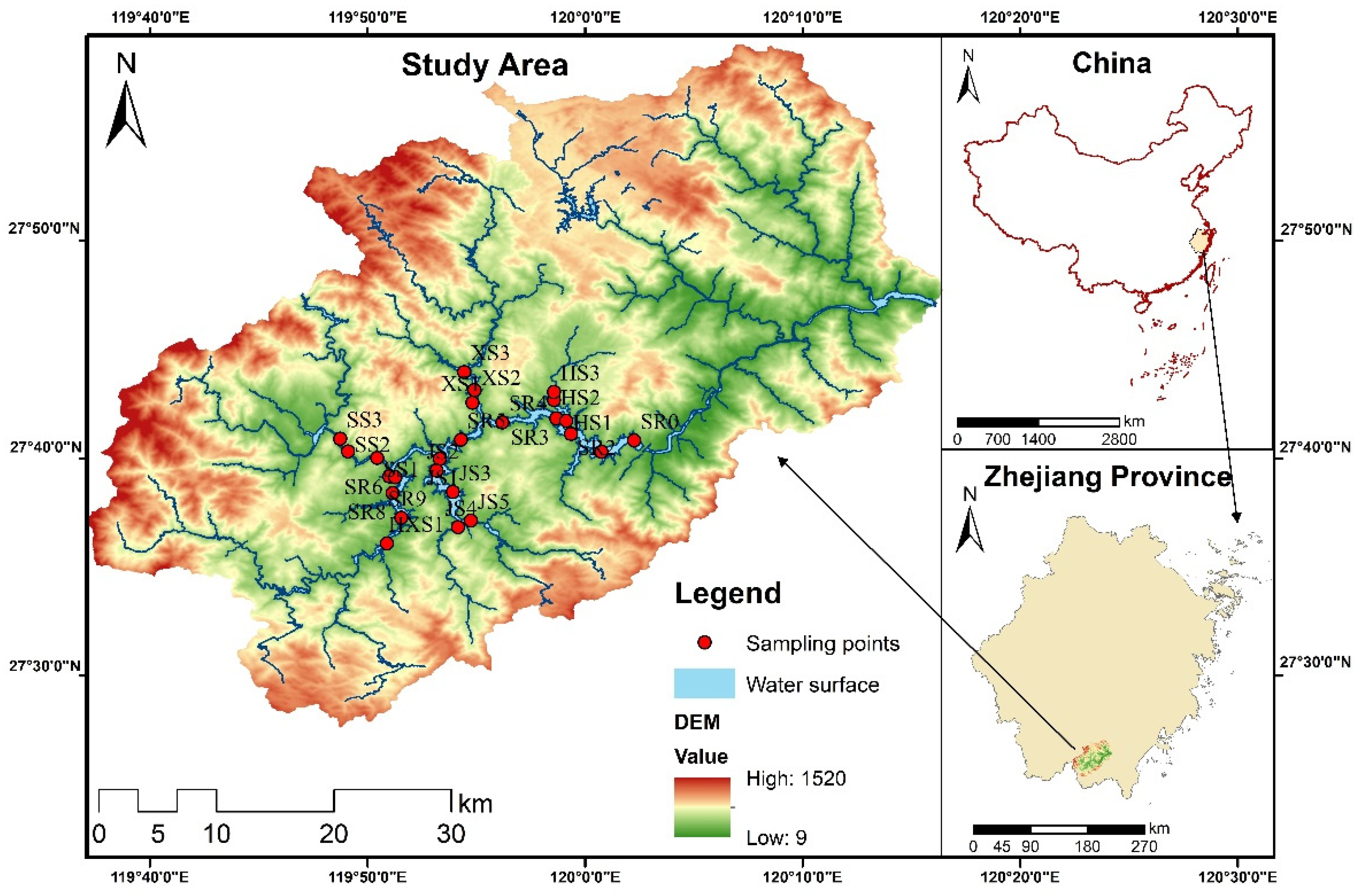
2.1. Description of the Study Area

Shanxi Reservoir (latitude 27°36′–27°50′; longitude 119°47′–120°15′), a large freshwater reservoir in the south of Zhejiang Province, is in the upper reaches of the Feiyun River, a typical river-type reservoir. It has a total reservoir capacity of 1.82 × 10⁹ m3 in a rainfall catchment area of 1529 km2, controlling nearly 80% of Wenzhou’s water resources, providing 1.34 × 10⁹ m3 of freshwater to Wenzhou’s urban area every year, supplying five million people in the water supply area and providing 2.20 × 10⁵ kW of peaking power to Wenzhou’s power grid, with obvious environmental and economic benefits. The Shanxi Reservoir is located in the subtropical monsoon climate zone, with an average multi-year precipitation of 1843.3 mm and an average multi-year temperature of 18.7 °C.

2.2. Sampling

For this study, based on the habitat and ecological characteristics of zooplankton [30], four seasons were selected for sampling; in April (spring), July (summer), October (autumn) in 2021, and January (winter) in 2022. As shown in Figure 1, 25 monitoring points were set up in the study area, according to the distribution of the main Shanxi Reservoir area and the tributary catchment area. According to the width of the section of different monitoring points set up with the bank perpendicular to the monitoring section, each monitoring section selected the mid-point and near-shore points for sampling.
According to the experience of relevant researchers, the distribution of the thermocline in lakes or oceans is generally used to determine the depth of samples to be collected at the corresponding sampling sites [40,41,42]. Water samples were collected from the upper layer (1 m), middle layer (4–7 m), and lower layer (10–20 m) using a 5 L water collector, considering the distribution of the thermocline in the study area.
Water environment indicators were obtained as follows. For the collected water samples on-site using DS5X (Hach Corporation) to measure water temperature (Tem), pH, dissolved oxygen (DO), electrical conductivity (EC), oxidation-reduction potential (ORP), and chlorophyll a (Chl-a), which are conventional indicators. For each layer of the sample retention volume of 10 L of water samples for the determination of routine water pollution indicators in the laboratory; according to the national standard (GB11892-89) [43] for the determination of permanganate index (CODMn) of environmental water quality. For the determination of total phosphorus (TP), the ammonium molybdate spectrophotometric method was used according to the national standard (GB11893-89) [44]. According to this, the determination of total nitrogen (TN) was carried out by UV spectrophotometric method using alkaline potassium persulfate elimination. The determination of ammonia nitrogen (NH3-N) in water samples was made according to the national standard (HJ535-2009) [45].
The zooplankton samples were obtained as follows: 10 L of water samples were collected from each layer, filtered using a 64μm pore size filter according to the national standard (SCT9402-2010) [46], the filter rinsed to obtain about 250 mL of zooplankton concentrate, and formaldehyde solution with a volume fraction of 5% was added for sample fixation. Zooplankton samples were classified and data collected in the laboratory using ZooScan, a zooplankton image acquisition system, in combination with imageJ image processing software and EcoTaxa 2.0 image analysis and processing website. Considering the accuracy of the ZooScan system for zooplankton monitoring and the related habits of zooplankton [47], the identification of zooplankton in the study area was completed with the assistance of OLYMPUS BX51 in this study.

2.3. Data Processing

In order to investigate the response between zooplankton and the water environment in Shanxi Freshwater Reservoir, the study area was divided into six sub-regions: the Shanxi Reservoir (SR), the Huangtankeng Stream (HS), the Xuezuokou Stream (XS), the Jujiangxi Stream (JS), the Sanchaxi Stream (SS), and the Hongkouxi Stream (HXS) according to the characteristics of the catchments in the study area. The screening of three representative zooplankton species based on the collected zooplankton samples gave results on the spatial and temporal heterogeneity of zooplankton in freshwater reservoirs. The results of the spatial and temporal heterogeneity of the water environmental factors of freshwater reservoirs were obtained by dividing them according to their physical, chemical, and ecological properties.
As the data in this study came from field sampling, there were a certain number of outliers, and to ensure better representativeness, the abnormal data were not presented. Correlations between three representative zooplankton species and 14 water environmental factors were analyzed using SPSS25 and Origin2021 using ANOVA and W-MERT methods respectively [48], and principal component analysis (PCA) was performed on each area of freshwater reservoirs in the study area to ensure that covariance matrices were characteristically decomposed with no or little loss of information, and multiple water environmental factors were generalized into representative major influences [49,50]. In addition, the relationship between zooplankton and water environmental factors was studied using detrended correspondence analysis (DCA) and redundancy analysis (RDA) using Canoco 5 software [51]. A cluster analysis, based on Euclidian distance, was used to check how Cladocera, Copepoda, and Rotifera were distributed along the study area using the sampling points and seasons of the reservoir as attributes [52]. A chi-square test was performed on the data for the water environment factors. One-way analysis of variance (ANOVA) was used for the normally distributed factors Tem, CODMn, pH, and TN to obtain significant differences in the spatial and temporal distribution of TN (ANOVA, p < 0.05). A Welch’s mean equality robustness test was applied to the non-normally distributed factors with uneven variances [53]. Finally, the results of spatial and temporal heterogeneity analysis of zooplankton and water environment factors were combined with data analysis methods to obtain the status of zooplankton and water environment in Shanxi Reservoir and to analyze their causes, and to explore the response relationship between typical zooplankton and water environment indicators.

3. Results

3.1. Spatial and Temporal Heterogeneity of Reservoir’s Water Environment

The variability of 12 water environmental factors in different areas of Shanxi Reservoir in terms of water temperature (Tem), electrical conductivity (EC), dissolved oxygen (DO), redox potential (ORP), pH, picocyanobacteria (PCY), turbidity (Tur), chlorophyll α (Chl-a), total nitrogen (TN), permanganate index (CODMn), total phosphorus (TP) and ammonia nitrogen (NH3-N) are presented in Table 1. After chi-square test and Welch’s mean equality robustness test, significant differences in the spatial and temporal distributions of EC, ORP, PCY, Chl-a, TP, and NH3-N (W-MERT, p < 0.05) were obtained. The 12 water environmental factors are further classified and discussed concerning their different properties.

3.1.1. Physicochemical Indicators of Water Bodies

The physical and chemical properties of water bodies are the basic components of the water environment and are a fundamental indication of the health of the water environment. Water temperature (Tem), turbidity (Tur), electrical conductivity (EC), pH, dissolved oxygen (DO), and redox potential (ORP)—these physical and chemical properties of water bodies are the basic components of the water environment and are a fundamental indication of the health of the water environment.
The study area is generally characterized by high water temperatures in summer and low water temperatures in winter. Combined with Figure 2 and the results presented by the data, the temporal and spatial differences in turbidity (Tur) and electrical conductivity (EC) in the study area were significant. The pH of the water bodies in the study area fluctuated significantly more in spring and summer than in autumn and winter, and the values increased significantly in summer. The spatial and temporal variability of dissolved oxygen (DO) in the water bodies of the study area was greatest in summer. The redox potential (ORP) also produced significant fluctuations and differences during the summer months.

3.1.2. Biological Indicators of Water Bodies

Similar to chlorophyll a (Chl-a), which is mainly derived from phytoplankton in the water, PCY values reflect the abundance of picocyanobacteria, which are typical of primary producers in the water environment of the study area.
According to the results of the Welch’s mean equality robustness test (W-MERT), Chl-a (W-MERT, p = 0.0001367 < 0.05) and PCY (W-MERT, p = 2.6499 × 10⁻¹³ < 0.05) showed highly significant differences in spatial and temporal distributions. In terms of temporal distribution, Chl-a and PCY were significantly less in winter than in other seasons; in terms of spatial distribution, Chl-a and PCY in spring showed higher levels in Huangtankeng Stream and Jujiangxi Stream than in other study areas. However, the Chl-a in summer showed a higher phenomenon in the Shanxi Reservoir than in the tributaries. In contrast, PCY was further elevated in number but spatially distributed more evenly than Chl-a.

3.1.3. Pollution Indicators of Water Bodies

Ammonia nitrogen (NH3-N) reflects the elemental nitrogen in water in the form of NH3 and NH 4 + . Total nitrogen (TN) contains various forms of nitrogen in the water body, and various forms of phosphorus elements in the water body are indicated by total phosphorus (TP). NH3-N, TN, and TP are mainly from domestic sewage and agricultural surface source pollution, and are important indicators of the health of water bodies. The permanganate index is a common indicator of oxidizable pollutants in water bodies. In terms of spatial and temporal distribution, TN (ANOVA, p = 0.0089 < 0.05), NH3-N (W-MERT, p = 0.006 < 0.05), and TP (W-MERT, p = 0.016 < 0.05) showed highly significant differences in spatial and temporal distribution.
In Figure 3, the amount of NH3-N in the water was significantly more in summer than in other seasons. TN and TP were higher than the yearly average in spring and summer, and CODMn was significantly less in winter than in other seasons. In addition, TN and NH3-N showed an increase in summer and a higher level in autumn. For the spatial distribution of pollution indicators, both TN and NH3-N showed extreme values in the Huangtankeng Stream, and fluctuated more between sub-regions within the same season; both CODMn and TP showed extreme values in the Shanxi Reservoir, but TP fluctuated more than CODMn within each sub-region.

3.2. Spatial and Temporal Heterogeneity of Reservoir’s Zooplankton

Through microscopic examination of zooplankton samples using OLYMPUS BX51, combined rapid statistical and technical work with the ZooScan zooplankton image scanning analysis system, 46 genus of zooplankton were identified at the genus level in accordance with the Atlas of Major Freshwater Zooplankton of Zhejiang Province (Drinking Water Sources) [54]. The detailed composition, frequency of recurrence and degree of dominance are shown in Table 2.
According to the data in Table 2, three of the genus Sinocalanus, Sinodiaptomus and Nitocra are prominent in terms of dominance of Copepoda, and Cladocera’s Macrothrix, Daphnia, Bosmina and Diaphanosoma all have a numerical dominance of more than 4%, significantly more than the other species, which further suggests that it is Cladocera and Copepoda that dominate the study area. Combining the information in Figure 4, in terms of temporal distribution, the number of zooplankton in the water column showed a gradual increase from spring to autumn and reached a maximum in summer and autumn, with a significant decrease after winter. In spring, the abundance of Cladocera fluctuated more in different subregions than Rotifera and Copepoda. All three orders in the same sub-region showed a greater increase in zooplankton abundance in summer compared to spring, with the mean abundance reaching its highest throughout the year. Copepoda was the dominant species within each subregion in summer under its abundance. The abundance of Cladocera in each subregion decayed with the onset of autumn but was generally much higher than in spring. The abundance of Rotifera and Copepoda in the Huangtanke Stream and Sanchaxi Stream sub-regions showed an increase compared to summer. The zooplankton abundance of the three orders showed a dramatic decrease in winter. The abundance of Rotifera and Cladocera in the Shanxi Reservoir sub-region decreased dramatically and was lower than the spring average. The abundance in the tributary sub-region decreased but overall was higher than the spring average. The Copepoda, the typical dominant zooplankton species in the study area during summer and autumn, had higher mean values in the study area than in spring, even though its abundance showed a dramatic decrease in winter.
In terms of spatial distribution, the following results can be obtained by comparing typical zooplankton abundances at different times during the same season. In spring, the average number of Rotifera in Shanxi Reservoir was lower than in the other five sub-regions. By contrast, the average number of Cladocera and Copepoda was higher than in the other five sub-regions. In summer, the average number of Rotifera and Cladocera in Shanxi Reservoir was lower than in the other five sub-regions, and the average number of Copepoda remained higher than the other five sub-regions. The average number of zooplankton decreased slightly in autumn compared to summer and generally showed a lower average number in Shanxi Reservoir than in the sub-region. The average number of zooplankton decreased further in winter, and the average number of Rotifera and Copepoda in Shanxi Reservoir was lower than the other five sub-regions, whereas the average number of Cladocera remained higher than the other five sub-regions.

3.3. Relationships between Water Environmental Factors and Zooplankton

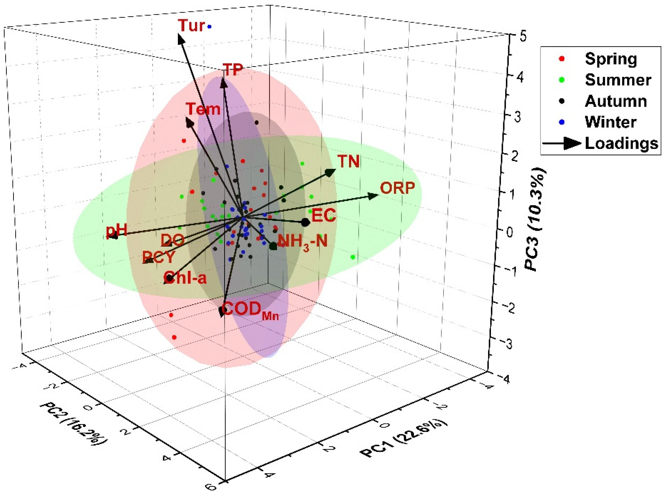
3.3.1. Principal Component Analysis (PCA)

Due to the large number of water environmental factors involved in this study, in order to facilitate the study of the response relationship between water environmental factors and zooplankton, after using the KMO (Kaiser-Meyer-Olkin) test for judgement (0 < 0.735 < 1), the dimensionality of the water environmental factors could be reduced using principal component analysis [55,56], and the loadings plot for the principal component analysis and the ellipses corresponding to the four 95% confidence levels for spring, summer, autumn and winter are shown in Figure 5.
For the water environment, the PCA of the 12 correlated variables resulted in three principal components (PC) that had eigenvalues >1 and accounted for 49.10% of the variance in the data. The first principal component (PC1) eigenvalue was 2.71 with a contribution rate of 22.60%, which accounted for the largest proportion of the variance, indicating that it had the strongest ability to combine the original variables. The water environment factors pH, Chl-a, CODMn, and Tem had larger weight coefficients, and pH had the largest weight coefficient and, very significantly, was positively correlated with the other three variables (p < 0.01). Therefore, PC1 could be synthesized as a chemical biological factor in water bodies. The second principal component (PC2) with an eigenvalue of 1.95 and a contribution of 16.22%, had the highest EC weight and the second highest TN weight. Very significantly, they were positively correlated (p < 0.01), so PC2 could be resolved as a physiochemical factor. The third principal component (PC3) had the largest Tur and TP weight, so PC3 could be resolved as a contamination risk factor.

3.3.2. Redundancy and Correlation Analysis

Before the constrained ranking analysis, the detrended correspondence analysis (DCA) of the principal water environmental factors was conducted. The results of the DCA analysis of the principal water environmental factors in all four seasons showed that the gradient length was less than 3, so the choice of redundancy analysis (RDA) was more reasonable [53]. Three major zooplankton taxa were used as forecast objects in the redundancy analysis, as well as eight principal water environmental factors as forecast factors. Clusters were determined based on a similarity matrix using Euclidian distance, with distances calculated by group-average sorting and ranked similarities. The water environmental factors involved in the analysis were screened using a Monte Carlo Permutation test (p < 0.05) and, combined with the results of the principal component analysis, the water environmental factors with explanatory value for each season were identified as Tem, Chl-a, pH, NH3-N, Tur, DO, TP and EC in spring, Tur, NH3-N, pH, Chl-a, DO, TP, EC, in summer ORP, EC, TN, pH, Chl-a, CODMn, DO, Tem in autumn, EC, Tur, pH, Chl-a, CODMn, Tem, DO in winter.
In spring, the eigenvalues for the first two axes of the RDA analysis were 0.247 and 0.121. From Figure 6a, it can be seen that EC, TN, CODMn, and NH3-N were positively correlated with Cladocera and Copepoda. The pH, Chl-a, and Tem were positively correlated with Rotifera, and ORP was negatively correlated with Rotifera. Cladocera formed good clusters with pH, Chl-a and EC, and Copepoda formed good clusters with Tur, TP and DO together with Rotifera. As the time enters summer, the total variation by RDA was 18.47, where the explanatory variables account for 62.80%. The pH, Chl-a, Tur, TP, Tem were positively correlated with Copepoda and Rotifera, and EC, TN were negatively correlated with them. pH, Chl-a, EC, TN, Tem were positively correlated with Cladocera. As shown in Figure 6b, Cladocera, Copepoda and Rotifera together formed good clusters with pH, Chl-a, Tur, TP, Tem. The three populations formed clusters with pH, Chl-a, Tur, TP, and Tem in summer to the results presented in the clustering heatmap in Figure 6b. In autumn, the eigenvalues for the first two axes of the RDA were 0.454 and 0.112, explaining 95.2% of the zooplankton variation. The pH, EC, Chl-a, TN, CODMn, Tem, NH3-N were positively correlated with Copepoda and Rotifera. pH, Chl-a, CODMn were positively correlated with Cladocera and EC, TN were negatively correlated with it. Cladocera, Copepoda, and Rotifera together formed good clusters with pH, Chl-a, TP, Tem, DO in Figure 6c. In winter, the species-environment correlation coefficients for RDA analysis were 0.757 and 0.419, respectively, indicating a significant correlation between water environmental factors and zooplankton. tur and TP were positively correlated with Cladocera, whereas EC, TN and CODMn, which were negatively correlated with Cladocera, were positively correlated with Copepoda and Rotifera. In addition, NH3-N was positively correlated with Copepoda, and pH and Chl-a were positively correlated with Rotifera. In Figure 6d, Cladocera, Copepoda and Rotifera together formed good clusters with Tur, TP and DO.

4. Discussion

The significant differences between the water level variation, water flow, and water connectivity of river-type reservoirs and natural water bodies lead to the aquatic ecosystems of river-type reservoirs being different from those of natural water bodies, and these differences also make the aquatic environment of reservoirs very fragile [50]. Because of this, a comprehensive evaluation of the water environment of river-type reservoirs and the health of the water ecology is essential to ensure water security and protect the ecosystem.

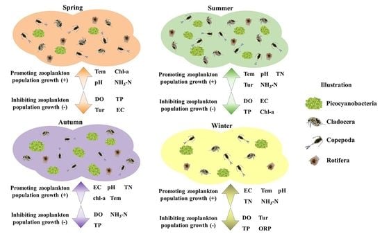
4.1. Factors Influencing Zooplankton Distribution

Our study found that the Shanxi Reservoir, a source of drinking water, is at some risk of contamination at certain times and locations. In fact, damming not only changes the connectivity of the river, but also alters the hydrodynamic conditions of natural water bodies, affecting their renewal cycles and making them more vulnerable to eutrophication risks [57,58]. Unlike previous studies [36], our study found that the PCY values in Huangtankeng Stream and Jujiang Stream in the study area were too high in summer, and the higher the PCY value, the greater the risk of algal blooms. According to research [59], local algal blooms will form in subtropical reservoirs when the density of blue-green algae is steadily higher than 50,000 cells/L. In Figure 3a,b, peaks in Chl-a and PCY are observed in Huangtankeng Stream and Jujiangxi Stream in spring and summer. And pH in these regions tended to be lower than in other regions during the same season. This is because, in addition to the obvious regional differences in pH distribution due to zonal factors, the horizontal distribution of pH is not entirely uniform in the same lake or water body due to environmental conditions such as incoming runoff, intensity of water exchange, and the number of biological populations in the lake [60]. Generally, in freshwater bodies, the pH level is related to the free carbon dioxide and dissolved carbonate ions in the lake water. Where the free carbon dioxide is high, the pH is low; the pH is correspondingly high in lakes with high content of bicarbonate ions and carbonate ions [61]. At the same time, lake algae generally consume free carbon dioxide in the water during their photosynthesis, increasing in pH response [62]. Our study also found that Tur and EC showed a large number of variations between seasons and spaces, as presented in Table 1 and Figure 2. Since the conductive particles in water bodies are mainly K+, Na+, Ca2+, Mg2+, Cl , SO 4 2 , HCO 4 2 and CO 3 2 , the total amount of these ions is close to the degree of mineralization of the water body, so the electrical conductivity is a side reflection of the degree of mineralization of the water body [63]. Turbidity can visually reflect the degree of turbidity of water bodies, which is mainly caused by insoluble sediment, humus, planktonic algae, colloidal particles, and other substances in the water bodies [64,65]. Dissolved oxygen did not show a large variability in spatial distribution in our study area, but showing fluctuations between seasons. Oxygen in water comes mainly from atmospheric dissolution and photosynthesis by aquatic organisms, and its content in water is influenced by temperature [66]. Notably, as presented in Figure 3c,d, our study found a high degree of variability in the spatial and temporal distribution of ammonia and total nitrogen, and the detection of ammonia and total nitrogen indicators compensated for the lack of relevant studies conducted by researchers on phytoplankton groups in the same area [36]. Nitrogenous compounds in natural water bodies often exist in three forms: ammonium nitrogen, nitrite nitrogen, and nitrate nitrogen, all of which can be used by aquatic organisms. When the water body is polluted or aquatic organisms die, organic nitrogen undergoes a series of decomposition to ammonia nitrogen form, then ammonia nitrogen is further oxidized to nitrite and finally to nitrate form [67]. Temperature is likewise an indicator of the large spatial and temporal variability within our study area. For the northern hemisphere, the lowest water temperature often occurs in January to February and the highest water temperature often occurs in July to August each year. The physiological and biochemical reactions in organisms change with temperature [68]. Within the appropriate temperature range, the physiological and biochemical reactions in organisms are accelerated with the increase in temperature, which promotes growth and development.
The results of our study indicate that the factors limiting the increase in zooplankton abundance in spring are mainly Tem and nutrient salts, which can be represented by PC1, PC2 in Figure 5. Comparing the observed data with the results of the RDA analysis, it is easy to see that the abundance of Rotifera is well explained by pH, Chl-a, and Tem, and that the abundance of Cladocera and Copepoda increases with EC, TN, NH3-N. In contrast to the previous study [69], the main factors limiting the increase in zooplankton abundance during summer are nutrient salinity, PCY and DO. The abundance of Rotifera and Copepoda increases with increasing pH, Chl-a, Tur, TP, Tem, and decreases with increasing EC, TN. The situation in autumn and winter is similar to previous studies [70], the main factors limiting the increase in zooplankton abundance in autumn are nutrient salinity and DO, which can be expressed by PC1, PC2. The abundance of Cladocera increases with pH, Chl-a. Similarly, within the appropriate range, increases in pH, EC, Chl-a, TN, CODMn, Tem, NH3-N result in a growing number of Copepoda and Rotifera. The main factors limiting the increase in abundance conferred on the animals in winter are nutrient salinity and PCY. The pH, Chl-a, EC, TN, and Tem predicted the abundance of Copepoda and Rotifera, and EC, TN, Tur, and TP were good predictors of Cladocera abundance. Another important finding was that zooplankton populations are influenced by different water environmental factors in different seasons, and they can also form good clusters with the corresponding water environmental factors under different conditions. Comparing the observed data with the results of the cluster analysis, it is easy to see that in spring the three zooplankton species form clusters with different water environmental factors, with Rotifera forming good clusters with NH3-N and DO, Cladocera with Tur, and Copepoda with EC, pH, and TP. In summer, when environmental conditions are favorable, the three zooplankton species form good clusters with pH, Chl-a, Tur, NH3-N, and DO. In autumn, the three zooplankton species form good clusters with pH, Chl-a, CODMn, ORP, and DO. In winter, when environmental conditions were harsh, the three zooplankton species formed good clusters with Tur, TP, Tem, Chl-a, and NH3-N, respectively.

4.2. Variation of Zooplankton Distribution

As shown in Table 2, we identified a variety of zooplankton in the study area, including 20 genus of Rotifera, 15 genus of Copepoda and 11 genus of Cladocera, all of which are common freshwater zooplankton in southeast China [71]. Although Rotifera species were more abundant, the crustaceans (Copepoda and Cladocera) were overwhelmingly dominant in terms of the number of individuals (79.8% of the microscopic samples), with a total of 30 genus with a reproduction rate of 60% or more, including 9 genus of Rotifera, 14 genus of Copepoda and 7 genus of Cladocera. The number of species with a numerical dominance of more than 1% was 5 genus of Rotifera, 13 genus of Copepoda, and 7 genus of Cladocera, respectively.
Previous research has focused more on zooplankton as indicators of water quality and for ecological assessment [19]. The formation of clusters between zooplankton and water environmental factors could be of interest in the future for ecological restoration and environmental monitoring. Similar to the results of other related studies [59,72], the nutrient levels in the study area were lower in spring than in summer and autumn, and levels of the water environment factors PCY and Chl-a, which measure biological indicators, were low in spring, suggesting that the primary producers, picocyanobacteria, as well as other algae, were less abundant in the water column. Tur, also a measure of suspended matter in the water column [65], was lower in spring than in other seasons, suggesting that the low levels of suspended particulate matter and organic detritus, in the water column limited the food sources of Copepoda and Cladocera, thus making differences in zooplankton abundance on a spatial scale less pronounced in spring.
The water temperature and solar radiation in the study area were significantly higher in summer and autumn than in spring and winter, and the suitable water temperature and solar radiation provided a good environment for the growth and development of algae, the producers located in the first trophic level in the study area [73]. Along with the algal blooms, Chl-a and PCY that could be detected in the water environment factors are increasing and zooplankton that feeds on algae and their metabolites are experiencing a peak in growth and reproduction [71], making the abundance of the three typical zooplankton species reach their maximums in spring and summer. The higher NH3-N content in the sub-regions of Huangtankeng Stream and Jujiangxi Stream provided sufficient nutrients for the growth and development of algae, making the Chl-a content in the sub-region of Huantankeng Stream much higher than that in other sub-regions, and likewise making the PCY content in the sub-region of Jujiangxi Stream much higher than that in other sub-regions.
In our study, variations of physicochemical indicators changed considerably with the seasons. The water temperature in autumn is between spring and summer, with more nutrient salts than in spring, making it more suitable for the growth and reproduction of producers such as algae. The values of PCY and Chl-a were correspondingly lower in Jujiangxi Stream, which had less TN and NH3-N, and higher in Huangtangkeng Stream, which had more TN and NH3-N. In the Shanxi Reservoir, which has a high TN content, the PCY values were higher than in the other sub-regions. Cladocera also occurs in abundance in the Jujiangxi Stream and Huangtangkeng Stream, areas of fertile water. Algae-feeding Copepoda were more abundant in Shanxi Reservoir, Jujiangxi Stream, and Huangtangkeng Stream than in the other sub-regions. Copepoda, which has a wide range of food sources [74], was significantly more abundant in Huangtankeng Stream than in the other regions.
Biological indicators in the study area were lower in winter than in summer and autumn, due to the amount of solar radiation, PCY and Chl-a were the lowest throughout the year. The life activities of aquatic organisms in the water column are somewhat restricted at this temperature [73], and the PCY and Chl-a in the water column are reduced to their lowest values throughout the year. Similarly, the decomposition of microorganisms is also restricted due to the temperature, causing the NH3-N content in the water column to decrease to some extent. More Copepoda spend the winter in the Sanchaxi Stream and Hongkouxi Stream, where Chl-a levels are high, and Cladocera spend the winter in sub-regions with slow flow conditions and rich nutrient salinity.

5. Conclusions

In the study area of Shanxi Reservoir, zooplankton showed the same spatial and temporal heterogeneity as the water environmental factors. Freshwater zooplankton, represented by Cladocera, Copepoda, and Rotifera showed not only clear seasonal differences in time, but also spatially variable response relationships with changes in key water environmental factors such as Tem, DO, nutrient salinity and EC. The main response relationships between water environmental factors and zooplankton exist in different seasons as follows. In spring, Tem and TP affect the number of Cladocera. EC, pH, and Tem affect the number of Copepoda, and pH, EC, and Chl-a affect the number of Rotifera. In summer, Tur, TP, and DO affect the abundance of Copepoda and Rotifera, and NH3-N affects the amount of Cladocera in the water. In autumn, Tem has an effect on the numbers of all three. Cladocera will be affected mainly by DO, and pH, EC will affect Copepoda numbers. Rotifera will also be affected mainly by EC in autumn. In winter, EC, pH, DO, TP affect the numbers of Copepoda and Rotifera. EC and Tur affect the number of Cladocera. Meanwhile, the three zooplankton species formed good clusters with pH, DO, Chl-a, and NH3-N during the summer months in abundant water, and with Tem, Tur, TP, and NH3-N during the winter months in dry water. This correspondence between zooplankton and relevant water environment factors in the respective seasons can be used not only to predict trends in water environment development but also as a key indicator of regional water environment deployment in the process of water diversion and storage during periods of abundance and drought.
Overall, the observations and analyses in this study suggest that temperature is a key factor influencing the differences in the spatial and temporal distribution of water environment and water ecology in riverine reservoirs. On the one hand, water temperature is a direct reflection of the intensity of solar radiation on the water body, and changes in water temperature can lead to changes in DO, EC, ORP, pH, Chl-a, PCY and other physicochemical and biological indicators. On the other hand, in the catchment area of river-type reservoirs, the change of temperature also indicates the change of seasons, which fits with the growth and development cycle of economic crops near the catchment area and economic fish in the reservoir. Nutrients such as nitrogen and phosphorus, as well as organic pollutants, will enter the reservoir with surface runoff, causing changes in chemical indicators. Changes in physical and chemical indicators will cause changes in biological indicators.
Due to the time and scale constraints, the analysis method in this study affected the generalizability of the results to a certain extent. In future studies, the assessment of the water environment and water ecological health of river-type reservoirs requires not only data support for a longer time series, but also data mining and the establishment and validation of models with relevant data in order to provide constructive evaluation and analysis of the water environment and water ecological health of other reservoirs with similar conditions using accurate and generalized models.

Author Contributions

Conceptualization, J.Y. and J.X.; methodology, W.C. and J.X.; software, J.Y.; validation, Y.W., R.Z. and X.D.; formal analysis, W.C.; investigation, J.Y., X.D. and Z.L.; resources, K.X.; data curation, Z.L.; writing—original draft preparation, J.Y. and J.X.; writing—review and editing, K.X.; visualization, Y.W.; supervision, Z.X.; project administration, Z.X., R.Z. and X.D.; funding acquisition, J.X. All authors have read and agreed to the published version of the manuscript.

Funding

This research was funded by the National Science and Technology Basic Resources Survey Special Project [Grant No. 2022FY100404], National Key Research and Development Program of China [Grant No. 2018YFD0900805], Key Program of Water Conservancy Science and Technology of Zhejiang Province [Grant No. RB1915], National Natural Science Foundation of China [Grant No. 41471069], Postgraduate Research and Practice Innovation Program of Jiangsu Province [Grant No. B200203137, KYCX20_0493], Fundamental Research Funds for the Central Universities [Grant No. B210203028].

Institutional Review Board Statement

Not applicable.

Informed Consent Statement

Not applicable.

Data Availability Statement

Not applicable.

Acknowledgments

The authors would like to thank BA students Shuyi Ji, Yuanshuo Lu, Zhengxin Wang, Chuwen Wang, MSc student Peng Zhang, Hao Wang, and Xiaohan Zhu of Hohai University for their field and laboratory contributions to this study. The authors are particularly grateful to Valerie Lopes and Tihana Mirkovic from York University, and Han Wang from Hong Kong University of Science and Technology for constructive advice during data analysis and visualization.

Conflicts of Interest

The authors declare no conflict of interest.

References

  1. Foley, J.A.; Ramankutty, N.; Brauman, K.A.; Cassidy, E.S.; Gerber, J.S.; Johnston, M.; Mueller, N.D.; O’Connell, C.; Ray, D.K.; West, P.C.; et al. Solutions for a Cultivated Planet. Nature 2011, 478, 337–342. [Google Scholar] [CrossRef] [PubMed] [Green Version]
  2. Steffen, W.; Richardson, K.; Rockstrom, J.; Cornell, S.E.; Fetzer, I.; Bennett, E.M.; Biggs, R.; Carpenter, S.R.; de Vries, W.; de Wit, C.A.; et al. Planetary Boundaries: Guiding Human Development on a Changing Planet. Science 2015, 347, 11. [Google Scholar] [CrossRef] [PubMed] [Green Version]
  3. Li, C.R.; Busquets, R.; Campos, L.C. Assessment of Microplastics in Freshwater Systems: A Review. Sci. Total Environ. 2020, 707, 12. [Google Scholar] [CrossRef] [PubMed]
  4. Acuna-Alonso, C.; Alvarez, X.; Lorenzo, O.; Cancela, A.; Valero, E.; Sanchez, A. Water Toxicity in Reservoirs after Freshwater Algae Harvest. J. Clean. Prod. 2021, 283, 104560. [Google Scholar] [CrossRef]
  5. Soares, L.M.V.; Calijuri, M.D. Deterministic Modelling of Freshwater Lakes and Reservoirs: Current Trends and Recent Progress. Environ. Model. Softw. 2021, 144, 16. [Google Scholar] [CrossRef]
  6. Zhang, Y.G.; Zhang, Z.; Xue, S.; Wang, R.J.; Xiao, M. Stability Analysis of a Typical Landslide Mass in the Three Gorges Reservoir under Varying Reservoir Water Levels. Environ. Earth Sci. 2020, 79, 14. [Google Scholar] [CrossRef]
  7. Hossain, M.; Huda, A.S.N.; Mekhilef, S.; Seyedmahmoudian, M.; Horan, B.; Stojcevski, A.; Ahmed, M. A State-of-the-Art Review of Hydropower in Malaysia as Renewable Energy: Current Status and Future Prospects. Energy Strategy Rev. 2018, 22, 426–437. [Google Scholar] [CrossRef]
  8. Kosek, K.; Ruman, M. Arctic Freshwater Environment Altered by the Accumulation of Commonly Determined and Potentially New Pops. Water 2021, 13, 1739. [Google Scholar] [CrossRef]
  9. Ji, B.; Liang, J.C.; Chen, R. Bacterial Eutrophic Index for Potential Water Quality Evaluation of a Freshwater Ecosystem. Environ. Sci. Pollut. Res. 2020, 27, 32449–32455. [Google Scholar] [CrossRef]
  10. Park, Y.; Lee, H.K.; Shin, J.K.; Chon, K.; Kim, S.; Cho, K.H.; Kim, J.H.; Baek, S.S. A Machine Learning Approach for Early Warning of Cyanobacterial Bloom Outbreaks in a Freshwater Reservoir. J. Environ. Manag. 2021, 288, 9. [Google Scholar] [CrossRef] [PubMed]
  11. Brack, W.; Ait-Aissa, S.; Burgess, R.M.; Busch, W.; Creusot, N.; Di Paolo, C.; Escher, B.I.; Hewitt, L.M.; Hilscherova, K.; Hollender, J.; et al. Effect-Directed Analysis Supporting Monitoring of Aquatic Environments—An in-Depth Overview. Sci. Total Environ. 2016, 544, 1073–1118. [Google Scholar] [CrossRef] [PubMed]
  12. Altenburger, R.; Brack, W.; Burgess, R.M.; Busch, W.; Escher, B.I.; Focks, A.; Hewitt, L.M.; Jacobsen, B.N.; de Alda, M.L.; Ait-Aissa, S.; et al. Future Water Quality Monitoring: Improving the Balance between Exposure and Toxicity Assessments of Real-World Pollutant Mixtures. Environ. Sci. Eur. 2019, 31, 17. [Google Scholar] [CrossRef] [Green Version]
  13. Sagan, V.; Peterson, K.T.; Maimaitijiang, M.; Sidike, P.; Sloan, J.; Greeling, B.A.; Maalouf, S.; Adams, C. Monitoring Inland Water Quality Using Remote Sensing: Potential and Limitations of Spectral Indices, Bio-Optical Simulations, Machine Learning, and Cloud Computing. Earth-Sci. Rev. 2020, 205, 31. [Google Scholar] [CrossRef]
  14. Shi, W.X.; Zhuang, W.E.; Hur, J.; Yang, L.Y. Monitoring Dissolved Organic Matter in Wastewater and Drinking Water Treatments Using Spectroscopic Analysis and Ultra-High Resolution Mass Spectrometry. Water Res. 2021, 188, 16. [Google Scholar] [CrossRef] [PubMed]
  15. Brooks, J.L.; Dodson, S.I. Predation, Body Size, and Composition of Plankton. Science 1965, 150, 28–35. [Google Scholar] [CrossRef] [PubMed]
  16. Elser, J.J.; Fagan, W.F.; Denno, R.F.; Dobberfuhl, D.R.; Folarin, A.; Huberty, A.; Interlandi, S.; Kilham, S.S.; McCauley, E.; Schulz, K.L.; et al. Nutritional Constraints in Terrestrial and Freshwater Food Webs. Nature 2000, 408, 578–580. [Google Scholar] [CrossRef]
  17. Frank, K.T.; Petrie, B.; Choi, J.S.; Leggett, W.C. Trophic Cascades in a Formerly Cod-Dominated Ecosystem. Science 2005, 308, 1621–1623. [Google Scholar] [CrossRef] [Green Version]
  18. Sousa, W.; Attayde, J.L.; Rocha, E.D.; Eskinazi-Sant’Anna, E.M. The Response of Zooplankton Assemblages to Variations in the Water Quality of Four Man-Made Lakes in Semi-Arid Northeastern Brazil. J. Plankton Res. 2008, 30, 699–708. [Google Scholar] [CrossRef] [Green Version]
  19. Jeppesen, E.; Noges, P.; Davidson, T.A.; Haberman, J.; Noges, T.; Blank, K.; Lauridsen, T.L.; Sondergaard, M.; Sayer, C.; Laugaste, R.; et al. Zooplankton as Indicators in Lakes: A Scientific-Based Plea for Including Zooplankton in the Ecological Quality Assessment of Lakes According to the European Water Framework Directive (Wfd). Hydrobiologia 2011, 676, 279–297. [Google Scholar] [CrossRef]
  20. Winder, M.; Schindler, D.E. Climate Change Uncouples Trophic Interactions in an Aquatic Ecosystem. Ecology 2004, 85, 2100–2106. [Google Scholar] [CrossRef]
  21. Ger, K.A.; Urrutia-Cordero, P.; Frost, P.C.; Hansson, L.A.; Sarnelle, O.; Wilson, A.E.; Lurling, M. The Interaction between Cyanobacteria and Zooplankton in a More Eutrophic World. Harmful Algae 2016, 54, 128–144. [Google Scholar] [CrossRef] [PubMed]
  22. Gallardo, B.; Clavero, M.; Sanchez, M.I.; Vila, M. Global Ecological Impacts of Invasive Species in Aquatic Ecosystems. Glob. Chang. Biol. 2016, 22, 151–163. [Google Scholar] [CrossRef] [PubMed]
  23. Jeppesen, E.; Brucet, S.; Naselli-Flores, L.; Papastergiadou, E.; Stefanidis, K.; Noges, T.; Noges, P.; Attayde, J.L.; Zohary, T.; Coppens, J.; et al. Ecological Impacts of Global Warming and Water Abstraction on Lakes and Reservoirs Due to Changes in Water Level and Related Changes in Salinity. Hydrobiologia 2015, 750, 201–227. [Google Scholar] [CrossRef]
  24. Miloslavich, P.; Bax, N.J.; Simmons, S.E.; Klein, E.; Appeltans, W.; Aburto-Oropeza, O.; Garcia, M.A.; Batten, S.D.; Benedetti-Cecchi, L.; Checkley, D.M.; et al. Essential Ocean Variables for Global Sustained Observations of Biodiversity and Ecosystem Changes. Glob. Chang. Biol. 2018, 24, 2416–2433. [Google Scholar] [CrossRef] [Green Version]
  25. Marcolin, C.R.; Lopes, R.M.; Jackson, G.A. Estimating Zooplankton Vertical Distribution from Combined Lopc and Zooscan Observations on the Brazilian Coast. Mar. Biol. 2015, 162, 2171–2186. [Google Scholar] [CrossRef]
  26. Wang, W.C.; Sun, S.; Zhang, F.; Sun, X.X.; Zhang, G.T. Zooplankton Community Structure, Abundance and Biovolume in Jiaozhou Bay and the Adjacent Coastal Yellow Sea During Summers of 2005-2012: Relationships with Increasing Water Temperature. J. Oceanol. Limnol. 2018, 36, 1655–1670. [Google Scholar] [CrossRef]
  27. Naito, A.; Abe, Y.; Matsuno, K.; Nishizawa, B.; Kanna, N.; Sugiyama, S.; Yamaguchi, A. Surface Zooplankton Size and Taxonomic Composition in Bow Doi N Fjord, North-Western Greenland: A Comparison of Zooscan, Opc and Microscopic Analyses. Polar Sci. 2019, 19, 120–129. [Google Scholar] [CrossRef]
  28. Wang, W.C.; Sun, S.; Sun, X.X.; Zhang, G.T.; Zhang, F. Spatial Patterns of Zooplankton Size Structure in Relation to Environmental Factors in Jiaozhou Bay, South Yellow Sea. Mar. Pollut. Bull. 2020, 150, 10. [Google Scholar] [CrossRef] [PubMed]
  29. Maas, A.E.; Gossner, H.; Smith, M.J.; Blanco-Bercial, L.; Irigoien, X. Use of Optical Imaging Datasets to Assess Biogeochemical Contributions of the Mesozooplankton. J. Plankton Res. 2021, 43, 475–491. [Google Scholar] [CrossRef]
  30. Noyon, M.; Poulton, A.J.; Asdar, S.; Weitz, R.; Giering, S.L.C. Mesozooplankton Community Distribution on the Agulhas Bank in Autumn: Size Structure and Production. Deep-Sea Res. Part Ii-Top. Stud. Oceanogr. 2022, 195, 15. [Google Scholar] [CrossRef]
  31. Garcia-Herrera, N.; Cornils, A.; Laudien, J.; Niehoff, B.; Hofer, J.; Forsterra, G.; Gonzalez, H.E.; Richter, C. Seasonal and Diel Variations in the Vertical Distribution, Composition, Abundance and Biomass of Zooplankton in a Deep Chilean Patagonian Fjord. Peerj 2022, 10, 31. [Google Scholar] [CrossRef] [PubMed]
  32. Schultes, S.; Lopes, R.M. Laser Optical Plankton Counter and Zooscan Intercomparison in Tropical and Subtropical Marine Ecosystems. Limnol. Oceanogr.-Methods 2009, 7, 771–784. [Google Scholar] [CrossRef]
  33. Dong, X.; Zhou, H. Calculation and Study of Total Nitrogen Influx Fluxes in Tributaries of Shanxi Reservoir. Zhejiang Hydrotech. 2017, 45, 22–24. [Google Scholar] [CrossRef]
  34. Li, A.L.; Haitao, C.; Yuanyuan, L.; Qiu, L.; Wenchuan, W. Simulation of Nitrogen Pollution in the Shanxi Reservoir Watershed Based on Swat Model. Nat. Environ. Pollut. Technol. 2020, 19, 1265–1272. [Google Scholar] [CrossRef]
  35. Chen, H.T.; Chen, J.; Liu, Y.Y.; He, J. Study of Nitrogen Pollution Simulation and Management Measures on Swat Model in Typhoon Period of Shanxi Reservoir Watershed, Zhejiang Province, China. Pol. J. Environ. Stud. 2021, 30, 2499–2507. [Google Scholar] [CrossRef]
  36. Yang, M.Z.; Xia, J.H.; Cai, W.W.; Zhou, Z.Y.; Yang, L.B.; Zhu, X.X.; Li, C.D. Seasonal and Spatial Distributions of Morpho-Functional Phytoplankton Groups and the Role of Environmental Factors in a Subtropical River-Type Reservoir. Water Sci. Technol. 2020, 82, 2316–2330. [Google Scholar] [CrossRef] [PubMed]
  37. Pianka, E.R. Niche Overlap and Diffuse Competition. Proc. Natl. Acad. Sci. USA 1974, 71, 2141–2145. [Google Scholar] [CrossRef] [PubMed] [Green Version]
  38. Xiong, W.; Huang, X.N.; Chen, Y.Y.; Fu, R.Y.; Du, X.; Chen, X.Y.; Zhan, A.B. Zooplankton Biodiversity Monitoring in Polluted Freshwater Ecosystems: A Technical Review. Environ. Sci. Ecotechnol. 2020, 1, 11. [Google Scholar] [CrossRef]
  39. Warren, J.D.; Leach, T.H.; Williamson, C.E. Measuring the Distribution, Abundance, and Biovolume of Zooplankton in an Oligotrophic Freshwater Lake with a 710 Khz Scientific Echosounder. Limnol. Oceanogr.-Methods 2016, 14, 231–244. [Google Scholar] [CrossRef] [Green Version]
  40. Sastri, A.R.; Gauthier, J.; Juneau, P.; Beisner, B.E. Biomass and Productivity Responses of Zooplankton Communities to Experimental Thermocline Deepening. Limnol. Oceanogr. 2014, 59, 1–16. [Google Scholar] [CrossRef]
  41. Gauthier, J.; Prairie, Y.T.; Beisner, B.E. Thermocline Deepening and Mixing Alter Zooplankton Phenology, Biomass and Body Size in a Whole-Lake Experiment. Freshw. Biol. 2014, 59, 998–1011. [Google Scholar] [CrossRef]
  42. Yaseen, T.; Bhat, S.U.; Bhat, F.A. Study of Vertical Distribution Dynamics of Zooplankton in a Thermally Stratified Warm Monomictic Lake of Kashmir Himalaya. Ecohydrology 2022, 15, 18. [Google Scholar] [CrossRef]
  43. GB11892-89; Water Quality-Determination of Permanganate index. Ministry of Environmental Protection of the People’s Republic of China: Beijing, China, 1989. (In Chinese)
  44. GB11893-89; Water Quality-Determination of Total Phosphorus-Ammonium Molybdate Spectrophotometric Method. Ministry of Environmental Protection of the People’s Republic of China: Beijing, China, 1989. (In Chinese)
  45. HJ535-2009; Water Quality-Determination of Ammonia Nitrogen-Nessler’s Reagent Spectrophotometry. Ministry of Environmental Protection of the People’s Republic of China: Beijing, China, 2009. (In Chinese)
  46. SCT9402-2010; Specifications for Freshwater Plankton Surveys. Ministry of Agriculture of the People’s Republic of China: Beijing, China, 2010. (In Chinese)
  47. Vogelmann, C.; Teichert, M.; Schubert, M.; Martens, A.; Schultes, S.; Stibor, H. The Usage of a Zooplankton Digitization Software to Study Plankton Dynamics in Freshwater Fisheries. Fish. Res. 2022, 251, 9. [Google Scholar] [CrossRef]
  48. Kumar, S.; Singh, R.; Singh, T.P.; Batish, A. On Mechanical Characterization of 3-D Printed Pla-Pvc-Wood Dust-Fe3o4 Composite. J. Thermoplast. Compos. Mater. 2022, 35, 36–53. [Google Scholar] [CrossRef]
  49. Sharma, A.S.; Gupta, S.; Singh, N.R. Zooplankton Community of Keibul Lamjao National Park (Klnp) Manipur, India in Relation to the Physico-Chemical Variables of the Water. Chin. J. Oceanol. Limnol. 2017, 35, 469–480. [Google Scholar] [CrossRef]
  50. Xiang, R.; Wang, L.J.; Li, H.; Tian, Z.B.; Zheng, B.H. Water Quality Variation in Tributaries of the Three Gorges Reservoir from 2000 to 2015. Water Res. 2021, 195, 12. [Google Scholar] [CrossRef]
  51. Tian, Z.Y.; Zheng, S.; Guo, S.J.; Zhu, M.L.; Liang, J.H.; Du, J.; Sun, X.X. Relationship between Zooplankton Community Characteristics and Environmental Conditions in the Surface Waters of the Western Pacific Ocean During the Winter of 2014. J. Ocean Univ. China 2021, 20, 706–720. [Google Scholar] [CrossRef]
  52. Lima, A.R.A.; Costa, M.F.; Barletta, M. Distribution Patterns of Microplastics within the Plankton of a Tropical Estuary. Environ. Res. 2014, 132, 146–155. [Google Scholar] [CrossRef]
  53. Wu, S.; Hua, P.; Gui, D.; Zhang, J.; Ying, G.; Krebs, P. Occurrences, Transport Drivers, and Risk Assessments of Antibiotics in Typical Oasis Surface and Groundwater. Water Res. 2022, 225, 119138. [Google Scholar] [CrossRef]
  54. Committee, E. Atlas of the Main Freshwater Zooplankton of Zhejiang Province (Drinking Water Sources); China Environment Publishing House: Beijing, China, 2013; Volume 445. (In Chinese) [Google Scholar]
  55. Olsen, R.L.; Chappell, R.W.; Loftis, J.C. Water Quality Sample Collection, Data Treatment and Results Presentation for Principal Components Analysis—Literature Review and Illinois River Watershed Case Study. Water Res. 2012, 46, 3110–3122. [Google Scholar] [CrossRef]
  56. ZerfaSs, C.; Lehmann, R.; Ueberschaar, N.; Sanchez-Arcos, C.; Totsche, K.U.; Pohnert, G. Groundwater Metabolome Responds to Recharge in Fractured Sedimentary Strata. Water Res. 2022, 223, 118998. [Google Scholar] [CrossRef] [PubMed]
  57. Yang, N.; Li, Y.; Zhang, W.L.; Lin, L.; Qian, B.; Wang, L.F.; Niu, L.H.; Zhang, H.J. Cascade Dam Impoundments Restrain the Trophic Transfer Efficiencies in Benthic Microbial Food Web. Water Res. 2020, 170, 115351. [Google Scholar] [CrossRef] [PubMed]
  58. Shi, X.; Sun, J.; Xiao, Z.J. Investigation on River Thermal Regime under Dam Influence by Integrating Remote Sensing and Water Temperature Model. Water 2021, 13, 133. [Google Scholar] [CrossRef]
  59. Yao, L.G.; Zhao, X.M.; Zhou, G.J.; Liang, R.C.; Gou, T.; Xia, B.C.; Li, S.Y.; Liu, C. Seasonal Succession of Phytoplankton Functional Groups and Driving Factors of Cyanobacterial Blooms in a Subtropical Reservoir in South China. Water 2020, 12, 1167. [Google Scholar] [CrossRef] [Green Version]
  60. Akis, S.; Ozcimen, D. Optimization of Ph Induced Flocculation of Marine and Freshwater Microalgae Via Central Composite Design. Biotechnol. Prog. 2019, 35, 6. [Google Scholar] [CrossRef]
  61. Gollnisch, R.; Alling, T.; Stockenreiter, M.; Ahren, D.; Grabowska, M.; Rengefors, K. Calcium and Ph Interaction Limits Bloom Formation and Expansion of a Nuisance Microalga. Limnol. Oceanogr. 2021, 66, 3523–3534. [Google Scholar] [CrossRef]
  62. Price, G.A.V.; Stauber, J.L.; Holland, A.; Koppel, D.J.; Van Genderen, E.J.; Ryan, A.C.; Jolley, D.F. The Influence of Ph on Zinc Lability and Toxicity to a Tropical Freshwater Microalga. Environ. Toxicol. Chem. 2021, 40, 2836–2845. [Google Scholar] [CrossRef]
  63. Assuncao, A.W.D.; Souza, B.P.; da Cunha-Santino, M.B.; Bianchini, I. Formation and Mineralization Kinetics of Dissolved Humic Substances from Aquatic Macrophytes Decomposition. J. Soils Sediments 2018, 18, 1252–1264. [Google Scholar] [CrossRef]
  64. Sosa-Aranda, I.; Zambrano, L. Relationship between Turbidity and the Benthic Community in the Preserved Montebello Lakes in Chiapas, Mexico. Mar. Freshw. Res. 2020, 71, 824–831. [Google Scholar] [CrossRef]
  65. Gozdziejewska, A.M.; Kruk, M. Zooplankton Network Conditioned by Turbidity Gradient in Small Anthropogenic Reservoirs. Sci. Rep. 2022, 12, 12. [Google Scholar] [CrossRef]
  66. Vad, C.F.; Horvath, Z.; Kiss, K.T.; Toth, B.; Pentek, A.L.; Acs, E. Vertical Distribution of Zooplankton in a Shallow Peatland Pond: The Limiting Role of Dissolved Oxygen. Ann. Limnol.-Int. J. Limnol. 2013, 49, 275–285. [Google Scholar] [CrossRef] [Green Version]
  67. Ding, S.; Dan, S.F.; Liu, Y.; He, J.; Zhu, D.D.; Jiao, L.X. Importance of Ammonia Nitrogen Potentially Released from Sediments to the Development of Eutrophication in a Plateau Lake. Environ. Pollut. 2022, 305, 11. [Google Scholar] [CrossRef] [PubMed]
  68. Pulsifer, J.; Laws, E. Temperature Dependence of Freshwater Phytoplankton Growth Rates and Zooplankton Grazing Rates. Water 2021, 13, 1591. [Google Scholar] [CrossRef]
  69. Amorim, C.A.; Moura, A.D. Ecological Impacts of Freshwater Algal Blooms on Water Quality, Plankton Biodiversity, Structure, and Ecosystem Functioning. Sci. Total Environ. 2021, 758, 13. [Google Scholar] [CrossRef] [PubMed]
  70. Burns, C.W.; Galbraith, L.M. Relating Planktonic Microbial Food Web Structure in Lentic Freshwater Ecosystems to Water Quality and Land Use. J. Plankton Res. 2007, 29, 127–139. [Google Scholar] [CrossRef]
  71. Li, C.C.; Feng, W.Y.; Chen, H.Y.; Li, X.F.; Song, F.H.; Guo, W.J.; Giesy, J.P.; Sun, F.H. Temporal Variation in Zooplankton and Phytoplankton Community Species Composition and the Affecting Factors in Lake Taihu-a Large Freshwater Lake in China. Environ. Pollut. 2019, 245, 1050–1057. [Google Scholar] [CrossRef]
  72. Huang, J.Y.; Wang, X.; Wang, X.Y.; Chen, Y.J.; Yang, Z.W.; Xie, S.G.; Li, T.T.; Song, S. Distribution Characteristics of Ammonia-Oxidizing Microorganisms and Their Responses to External Nitrogen and Carbon in Sediments of a Freshwater Reservoir, China. Aquat. Ecol. 2022, 56, 841–857. [Google Scholar] [CrossRef]
  73. Rhode, S.C.; Pawlowski, M.; Tollrian, R. The Impact of Ultraviolet Radiation on the Vertical Distribution of Zooplankton of the Genus Daphnia. Nature 2001, 412, 69–72. [Google Scholar] [CrossRef]
  74. Diniz, L.P.; Franca, E.J.; Bonecker, C.C.; Marcolin, C.R.; De Melo, M. Non-Predatory Mortality of Planktonic Microcrustaceans (Cladocera and Copepoda) in Neotropical Semiarid Reservoirs. An. Acad. Bras. Cienc. 2021, 93, 16. [Google Scholar] [CrossRef]
Figure 1. Sampling points in the Shanxi reservoir.
Sustainability 14 13719 g001
Figure 2. Plumbline diagrams of the spatial and temporal distribution of physical and chemical properties of water bodies in the study area in different seasons: (a) Spring; (b) Summer; (c) Autumn; (d) Winter.
Sustainability 14 13719 g002aSustainability 14 13719 g002b
Figure 3. Stacked bar charts of the spatial and temporal distribution of water environmental factors: (a) Chl-a; (b) PCY; (c) NH3-N; (d) TN; (e) CODMn; (f) TP.
Sustainability 14 13719 g003
Figure 4. Three-dimensional dotted waterfall maps of the spatial and temporal distribution of plankton and images from OLYMPUS BX51 and ZooScan scans of (a) Cladocera; (b) Copepoda; (c) Rotifera.
Sustainability 14 13719 g004aSustainability 14 13719 g004b
Figure 5. Loadings of principal component analysis of water environment factors.
Sustainability 14 13719 g005
Figure 6. Plot of principal components with zooplankton redundancy analysis and clustering heatmap in different seasons: (a) Spring; (b) Summer; (c) Autumn; (d) Winter.
Sustainability 14 13719 g006aSustainability 14 13719 g006b
Table 1. Water Environment in the Study Area.
RegionShanxi
Reservoir
(SR)
Huangtankeng Stream
(HS)
Xuezuokou Stream
(XS)
Jujiang
Stream
(JS)
Sanchaxi
Stream
(SS)
Hongkouxi Stream
(HKS)
Water
Environment
Tem
(°C)
15.30~31.22 ^15.47~29.0815.59~30.9115.84~31.0015.84~31.0016.21~31.02
(22.67 ± 5.06) *(22.39 ± 5.11)(22.80 ± 5.34)(23.43 ± 4.99)(22.95 ± 4.96)(23.90 ± 6.06)
EC
(mS/cm)
31.16~47.6040.70~66.6031.42~46.2032.90~70.0035.13~52.2037.40~47.40
(42.60 ± 4.05)(50.60 ± 4.11)(41.01 ± 5.08)(46.71 ± 10.37)(43.19 ± 5.32)(44.70 ± 4.88)
DO
(mg/L)
5.07~8.165.14~8.325.84~7.695.25~7.755.26~8.486.08~8.48
(6.78 ± 0.86)(6.88 ± 1.06)(6.99 ± 0.70)(6.84 ± 0.81)(7.02 ± 0.82)(7.30 ± 1.00)
ORP
(V)
0.19~0.460.34~0.520.18~0.440.14~0.430.16~0.460.20~0.43
(0.37 ± 0.07)(0.40 ± 0.05)(0.37 ± 0.08)(0.33 ± 0.10)(0.35 ± 0.11)(0.35 ± 0.10)
pH6.43~8.176.81~7.886.49~8.236.54~8.026.68~8.137.15~8.10
(7.21 ± 0.43)(7.29 ± 0.30)(7.20 ± 0.50)(7.34 ± 0.43)(7.36 ± 0.49)(7.43 ± 0.45)
PCY
(×103 cell/L)
0.38~19.380.38~19.370.53~3.990.67~19.380.74~10.030.95~4.90
(2.05 ± 1.56)(2.05 ± 1.56)(2.02 ± 1.47)(5.27 ± 4.74)(3.87 ± 3.04)(3.33 ± 1.71)
Tur
(NTU)
1.10~8.003.40~6.202.60~5.301.50~7.951.70~11.101.90~9.90
(4.34 ± 1.75)(4.71 ± 0.89)(4.36 ± 0.87)(4.14 ± 1.79)(5.13 ± 2.55)(5.44 ± 3.62)
Chl-a
(mg/L)
0.60~4.161.24~13.660.63~7.540.50~4.791.20~6.281.05~3.58
(1.71 ± 1.11)(4.09 ± 3.50)(2.13 ± 2.43)(2.31 ± 1.52)(2.85 ± 1.61)(2.43 ± 1.25)
TN
(mg/L)
0.10~0.630.30~0.670.2282~0.47540.14~0.470.07~0.460.17~0.49
(0.38 ± 0.12)(0.44 ± 0.12)(0.35 ± 0.065)(0.33 ± 0.096)(0.31 ± 0.14)(0.36 ± 0.14)
CODMn
(mg/L)
0.37~2.000.72~2.300.73~1.880.75~1.800.63~1.700.78~1.89
1.36 ± 0.43(1.58 ± 0.53)(1.42 ± 0.37)(1.42 ± 0.35)(1.35 ± 0.43)(1.53 ± 0.51)
TP
(μg/L)
6.10~128.404.40~40.006.10~128.406.50~36.008.30~38.8010.60~30.30
(23.90 ± 23.80)(20.90 ± 12.30)(23.91 ± 23.82)(22.90 ± 9.50)(23.20 ± 11.10)(21.30 ± 9.70)
NH3N
(μg/L)
13.10~174.307.90~235.1011.80~118.6010.20~155.803.20~143.003.00~170.00
(50.20 ± 42.40)(78.30 ± 74.90)(37.70 ± 36.30)(52.40 ± 54.30)(60.30 ± 46.10)(76.20 ± 66.50)
^ indicates the range of an indicator. * Mean values and standard deviations (SD) are shown in parentheses.
Table 2. The species composition and individual dominance of the study area.
Categories
(Orders)
Name of the Species (Genus)Frequency of
Recurrence *
Degree of DominanceName of the Species (Genus)Frequency of RecurrenceDegree of Dominance
RotiferaAsplanchna100%2.60%Keratella40%0.20%
Polyarthra80%4.31%Testudinalla40%0.60%
Trichocerca60%0.25%Filinia40%0.53%
Gastropus60%0.44%Ascomorpha40%0.33%
Mytilina60%0.49%Eosphora40%0.63%
Brachiomus60%3.07%A.fissa20%0.02%
Cephalodella60%3.72%Rotaria20%0.26%
Pompholyx60%1.16%Epiphanes20%0.42%
Synchaeta60%0.34%Euchlanis20%0.02%
Notholeca40%0.74%Ploesoma20%0.06%
CopepodaNitocra100%6.90%Paracyclops80%2.58%
Sinocalanus100%11.80%Mesocyclops80%1.99%
Sinodiaptomus100%9.00%Heliodiaptomus80%5.39%
Cyclops100%1.51%Onchocamptus60%0.15%
Tropocyclops80%2.12%Limnoithona60%1.06%
Themocyclops80%2.23%Neodiaptomus60%1.64%
Canthocamptus80%1.47%Macrocyclops40%0.05%
Mongolodiaptpmus80%1.00%
CladoceraMacrothrix100%4.20%Diaphanosoma60%5.60%
Daphnia80%6.12%Camptocercus40%0.49%
Bosminopsis60%1.37%Leydigia20%0.24%
Chydorus60%3.54%Alona20%0.32%
Simocephalus60%2.11%Moinodaphnia20%0.08%
Bosmina60%6.92%
* Probability of being observable in a single survey cycle.
Publisher’s Note: MDPI stays neutral with regard to jurisdictional claims in published maps and institutional affiliations.

