A Study of the Impacts of Air Pollution on the Agricultural Community and Yield Crops (Indian Context)

Abstract

Air pollution has been an vital issue throughout the 21st century, and has also significantly impacted the agricultural community, especially farmers and yield crops. This work aims to review air-pollution research to understand its impacts on the agricultural community and yield crops, specifically in developing countries, such as India. The present work highlights various aspects of agricultural damage caused by the impacts of air pollution. Furthermore, in the undertaken study, a rigorous and detailed discussion of state-wise and city-wise yield-crop losses caused by air pollution in India and its impacts has been performed. To represent air-pollution impacts, the color-coding-based AQI (Air Quality Index) risk-classification metrics have been used to represent AQI variations in India’s agrarian states and cities. Finally, recent impacts of air pollution concerning AQI variations for May 2019 to February 2020, Seasonal AQI variations, impacts of PM${}_{2.5}$, and PM${}_{10}$ in various agrarian states and India cities are presented using various tabular and graphical representations.

1. Background and Motivation

Several scientists are actively involved in the environmental monitoring field due to their concern over this critical problem. In [1], the authors conducted a detailed review of acute respiratory infections due to burning from an Indian perspective using satellite and national-health survey data. The primary purpose of this study was to analyze economic and health-related costs in Northern India. In [2], the authors highlighted that respiratory diseases are considered as the leading causes of deaths of farmers. The study focused on the respirable air particles released by agricultural crop-residue burning (ACRB) and found the burdens caused by it. The statistics gathered point to a large investment gap in the agriculture sector. Stopping farmers from burning stubble and finding alternative crop-residue disposal solutions is the key, eventually catering to an improvement in population-level respiratory health. This study shows how large an impact wrongful crop-burning techniques have on farmer mortality and general-population mortality rates. The effects of air pollution on the world community are well established. However, it can significantly affect food crop yields and their nutritional quality and safety, which are essential for food security crops. In developing countries such as India, air pollution halved the yield of wheat and rice crops. Recently, cultural and adversarial actions have led to a new peak in pollution levels around the globe and specifically in India, which has spread toward rural areas where primary agricultural activities are conducted, affecting farmers’ lifespans. The cause of air pollution is mainly emissions from industrial sources, power generation, waste disposal, the operation of internal combustion engines, and the burning of stubbles and paddies. Air pollutants, such as particulate matter and liquid and solid wastes, can cause health hazards, such as sinusitis, asthma, organic dust toxic syndrome, nasal irritation, central nervous system symptoms, and death [3,4,5,6,7,8]. Approximately 2.5 million farmers on the Indo-Gangetic plain grow two crops per year in India: rice and wheat. Rice is grown in such a manner that its water needs are met by the rainy season, such that in a short period of 10 to 20 days, the fields are cleared of wheat. One of the critical issues in this situation is the domestic burning of biofuels, which causes more deaths than deaths due to industrial outages [9,10,11,12].

Figure 1a,b represent the impact that air pollution has on farming land and crops. With farmers forced to burn the stubble of their harvested crops each year, the agriculture sector contributes equally, if not more, to the pollution that affects the country [13]. Farmers must burn paddy fields to dispose of stubble after harvesting because they have no other option. Farmers resort to burning stubble as it is easy and requires minimal costs. Hiring combine harvesters is an option, but most farmers reject this to avoid any extra costs. Stubble burning renders the soil less fertile, such that farmers compensate for this loss of fertility by using more fertilizers, water, and power for the same area [14]. This creates a chain reaction of more pollution, less fertile land, zero technological improvements, and increased mortality and morbidity rates. If more sustainable production methods are used, agriculture’s adverse effects on the environment can be seen. In fact, in some cases, agriculture plays a vital role in repelling them, for example, by storing carbon in the soil, increasing water infiltration, and preserving rural landscapes and biodiversity [15]. Livestock accounts for 40 percent of global emissions, mineral fertilizers 16 percent, and biomass burning and crop residues 18 percent. Burning plant biomass is another primary air-pollutant source, including carbon dioxide, nitrous oxide, and smoke particles. Humans are estimated to burn 90 percent of the biomass, primarily through deforestation and deforestation, by deliberately burning down forest vegetation with forage residues [6,16,17].

Therefore, drafting communication strategies that involve access to information on no-burn alternatives is necessary. Due to prolonged exposure to pesticides and fertilizers, airborne emissions emitted by the air cause numerous health-related issues for these farmers [18]. Therefore, the loss of biodiversity is not limited to the land-clearing phase of agricultural development but may persist for a very long time. The most common respiratory diseases in farmers are acute bronchitis (for swine confinement workers), asthma exacerbation, chronic obstructive pulmonary disease (COPD) (chronic exacerbation), mucous membrane irritants (sick-building syndrome), and organic dust toxic syndrome (ODTS). These infections are the result of exposure to gases, such as nitrogen dioxide (NO₂), hydrogen sulfide (H₂S), ammonia (NH₃), carbon dioxide (CO₂), methane (CH₄), and sulfur dioxide (SO₂) [19,20]. India is an agricultural economy, which indicates that it relies heavily on the agricultural industry for its surplus and its main component of producing agricultural land. Livestock farming and crop production are the main agricultural activities in India. Agro-industry input mainly focuses on the raw materials used in agricultural production, including the input of native and chemical components, agricultural fields, and equipment [21,22,23]. Various types of chemical applications, such as chemical fertilizers, pesticides, and food additives, in agricultural production exhibit different agricultural outcomes. The use of pesticides and fertilizers plays a significant role in increasing agricultural production and ensuring agricultural products. Fertilizer provides a variety of nutrients needed for crop growth and increases production. Pesticides reduce the economic costs of pests, plant diseases, and weeds during agricultural production. However, numerous scientists have reported on the harmful residues from agricultural chemicals in the air, soil, water, and even in human blood and adipose tissue [24,25,26,27,28,29,30]. Previous studies have shown that the excessive use of inorganic fertilizers causes the accumulation of pollutants, such as As, Cd, F, Pb, and Hg, in soils [31]. This is consistent with findings showing that external pesticide use significantly impacts air pollution within agricultural communities [32], shown in Toxic Air reports, (https://www.greenpeace.org/southeastasia/press/3594/toxic-air-the-price-of-fossil-fuels/, accessed on 4 September 2022).

As the fifth-largest cause of death in India, with an estimated death toll of approximately 620,000, we must emphasize external pollution as an important factor [33]. External pollution kills more people every year than household pollution and affects the overall pollution index [34,35,36,37,38]. The highest level of pollution from the agricultural sector is derived from methane, ammonia, and carbon dioxide. Agricultural activities that generate ammonia in the atmosphere accounted for 83% of the total air pollution from agriculture in 2015. The agricultural sector is polluting the environment, where grain and oil crops appear to be the culprit [39]. This can be explained by extensive agricultural practices and process machinery (i.e., gasoline, fuel, oil, and preparation). The resulting pollution in agriculture can affect people in different professions, and living or working in neighboring towns or cities, typical for India’s northern regions. With the agricultural climate and harvesting in Uttar Pradesh, Haryana, and Punjab, there are significant changes in the Air Quality Index of Delhi, which is due to fluctuations in the average CH₄ and NO₂ concentrations of the atmosphere. This leads to bad air quality for people living in these areas. Thus, external air quality has become a significant concern for the public and policymakers [40].

Table 1. A list of used terminologies.

Risk Classification	AQI Values
AQI	Air Quality Index
PM${}_{2.5}$	Particulate matter 2.5
PM${}_{10}$	Particulate matter 10
NO${}_2$	Nitrogen dioxide
CH${}_4$	Methane
H${}_2$S	Hydrogen sulphide
O${}_3$	Ozone
As	Arsenic
Cu	Copper
HG	Mercury
SO${}_2$	Sulfur dioxide
WHO	World Health Organization

represents a list of terminologies used in the conducted experiments.

2. Related Work

Fatmi et al. [41] analyzed black carbon’s impacts on urban atmospheres in Southeast Asia regions. Cristina et al. [42] discussed the diverse impacts of black carbon on the surrounding environment and its health-related risks in various Thailand regions. This study shows black carbon, a heavy pollutant in the region, causing a much larger problem. Similarly, in India, PM${}_{2.5}$ and PM${}_{10}$ have been the major pollutants, which have their health-related risks. A review on paddy and wheat stubble blazing has been conducted for various regions of India. Marks et al. [43] revealed that the burning of biomass not only affects climate conditions, but it also damages plant nutrients. In this study, the environmental cost of paddy straw burning in northwest India was calculated. The west is the country’s major crop producer and contributes to India’s rising pollution problems. This study helps us focus on India’s major cities and gives the statistical information about the cost-effectiveness of current crop-burning techniques. In conclusion, we find how the social cost of burning per annum in the region is extreme. The ecosystem there is deprived of other important improvements due to incorrect burning techniques. Zhang et al. [44] reviewed livestock- and cropland-related data to reduce the effects of agriculture-based pollution in China. North et al. [45] conducted a review which discusses the benefits of excretion nitrogen on human health and food security. The review also discussed the ways of mitigating agricultural pollution using excretion nitrogen. Daxini et al. [45] reviewed farmer characteristics to identify good health practices for farmers’ wellbeing. The review also describes how better nutrient management can mitigate the risk of nutrient loss to the surrounding environment. This study, performed in Ireland, focuses on optimizing resource use efficiency. Improper management of agricultural production can lead to an increased risk of the loss of natural resources in the environment; this study helps us establish important future directions for the use of this review paper (CPCB reports, https://cpcb.nic.in/about-namp/, accessed on 4 September 2022). Zhang and Cao [2] proposed methods to manage PM${}_{2.5}$ pollution due to biomass burning in China. This study also revealed that the China government has taken proactive steps in rural and urban regions to mitigate biomass-burning emissions. The study also discussed the negative impacts of biomass burning in increasing local and regional pollution risks in China. Chin et al. [46] found that China and India have a common major pollutant, PM${}_{2.5}$, and this study covers multiple solutions, which can be used in India after PM${}_{2.5}$ concentration levels are controlled. Chen et al. [47,48] analyzed the effects of air pollution in China and its impact on health and stroke mortality. The undertaken study focused on the impacts of PM${}_{10}$ in eight cities of China. Christidis et al. [49] analyzed the impacts of PM${}_{2.5}$ in the surrounding environment and mortality analysis of the Canadian community. He et al. [50] discussed the impacts of a particular matter (PM${}_{2.5}$) in various Canadian regions and deaths due to air pollution. Chen et al. [3] reviewed PM${}_{2.5}$ concentrations and their impacts, as well as performing a mortality analysis of cardiovascular diseases. This study also proposed a component-adjustment approach to estimate and measure the impacts of PM${}_{2.5}$ on people’s health. This study also discussed the causes of air-pollution-related cardiovascular diseases. Amsalu et al. [51] performed a detailed analysis of air-pollution-related deaths and diseases.

All these studies have a common major pollutant, PM${}_{2.5}$. Considering the impacts it has had on people’s health in other countries, India should take this as a warning and focus on mitigating these issues. These studies set a bar for our review work, focusing on the ultimate goal, mortality analysis, and health impacts due to air pollution on the global community and India. Lasko and Vandrevu [52] conducted air-quality assessments in Vietnam by considering rice-residue-burning emissions estimates. The Atlan Reports (https://blog.atlan.com/announcements/tracking-air-pollution-in-delhi/, accessed on 4 September 2022) reveal that the rice residues are burned to prepare the agricultural field for the upcoming season after completing the hand-harvesting process. This study highlighted that rice-residue burning directly impacts the air pollution in the Southern part of Asia and Vietnam. Cambra-Lopez et al. [53] conducted a review of airborne particulate matter originating from livestock materials. Beckett et al. [54] investigated vegetation and urban woodlands’ roles in mitigating air pollution’s particulate matter effects. Pani et al. [55] reviewed seasonal air-pollution impacts and Rico et al. [56] conducted a detailed review of various risks involved with cage farming in Thailand. Zanobetti et al. [57] examined the association between ozone and mortality in 20 countries. The global impact of air pollution is determined in this study. With the 20 countries being the major producers of crops in their respective regions, the air pollution created is primarily due to agricultural disadvantages. Brown et al. [58] performed a detailed study of PM${}_{2.5}$ and mortality of Indian citizens. This study measures PM${}_{2.5}$ in North Indian regions and proves how India’s citizens are exposed to higher PM${}_{2.5}$ levels than advised. The study concludes that India has disproportionately high mortality and disease burden due to air pollution. This burden is usually higher in lower SDI studies in northern India. Reducing the inevitable fatalities and deaths from disease burden from this great environmental disaster is based on the rapid implementation of a cohesive policy across India coupled with the severity of air pollution in each province. Huang et al. [59,60] investigated the mortality of U.S. citizens, as well as performing a risk analysis of non-accidental and heart-related problems. Swaminathan [61] discussed the concept of biodiversity to mitigate environmental pollution.

Agudelo-Castaneda et al. [62] analyzed the effects of hydrocarbons on urban environments and respiratory health risks. Mills and Lee [63] analyzed threats associated with carbapenem bacteria in surrounding environments and reservoir contamination. With advancements in wireless sensor networks, sensing technology, and the Internet of Things, previous studies attempted to implement air-quality monitoring systems to measure various air-quality parameters. Al-Haija et al. [64] and Kularatna and Sudantha [4] implemented a microcontroller-based system using general-purpose gas sensors. The Environmental Air Pollution Monitoring System (EAPMS) developed here uses semiconductor sensors to measure the concentration of gases CO, NO, SO, and O. In addition, EAPMS can provide warnings when pollution levels exceed predetermined maxima. The system can be translated to a lower version for developing countries. Al-ali et al. [65] and Devarakonda et al. [7] established and tested a distributed pollution monitoring system using the general packet radio services (GPRS) public network. Pollution data from various mobile sensor arrays were transmitted to a central local server. SocialCops is a data intelligence company located in India that has developed a project to measure Delhi’s air pollution. This project module comprises sensors, a global positioning system (GPS) shield, and a GPRS shield. Using this approach, data is transmitted on the GPRS network. Abraham and Li [66] developed a system that measures indoor levels of CO, ozone, and CO₂ using the ZigBee mesh network. Kumar et al. [67], Ferdoush and Li [68], and Bacco et al. [69] all implemented monitoring systems of air-pollution parameters. A gas sensor-based embedded system was developed. In this approach, the CNT-based gas sensor was developed, and the MSP430 controller was used to detect ammonia. Tiwari et al. [70] developed a system to monitor methane, temperature, and humidity using Raspberry Pi, which communicates received data to a local webserver. This approach was implemented at the Bits Pilani research lab in India. Marques et al. [71] developed an air-quality monitoring system for ambient assisted living. The system is designed to monitor liquified petroleum gas (LPG) using an MQ6 sensor connected to a data transmission laptop. Dhingra et al. [72], Huang et al. [60], and Sun and Zhu [73] proposed designs for wireless mobile air-pollution monitoring applications using cloud-based services to acquire data cost-effectively with low-cost sensors. In India, the Central Pollution Control Board has implemented a nationwide program known as the National Air Quality Monitoring Programme (NAMP Reports, http://cpcbenvis.nic.in/airpollution/finding.html, accessed on 4 September 2022) for ambient air-quality monitoring. This program manages a network consisting of 779 fixed operating stations across various cities of India. The Indian government encourages and funds projects related to air-quality pollution in light of the alarming situations in cities such as Delhi, Ahmedabad, Kolkata, Mumbai, and Pune. The Indian government has also developed a portal (www.aqi.in, accessed on 4 September 2022) that provides real-time monitoring of the AQI, PM${}_{2.5}$, and PM${}_{10}$ parameters. This article is organized as follows. Section 3 presents a review of the state-of-the-art methodologies. Section 4 discusses the results and discussions about air-pollution impacts on yield crops, agrarian states, and cities; Section 5 presents our concluding remarks and future recommendations.

3. Materials and Methods

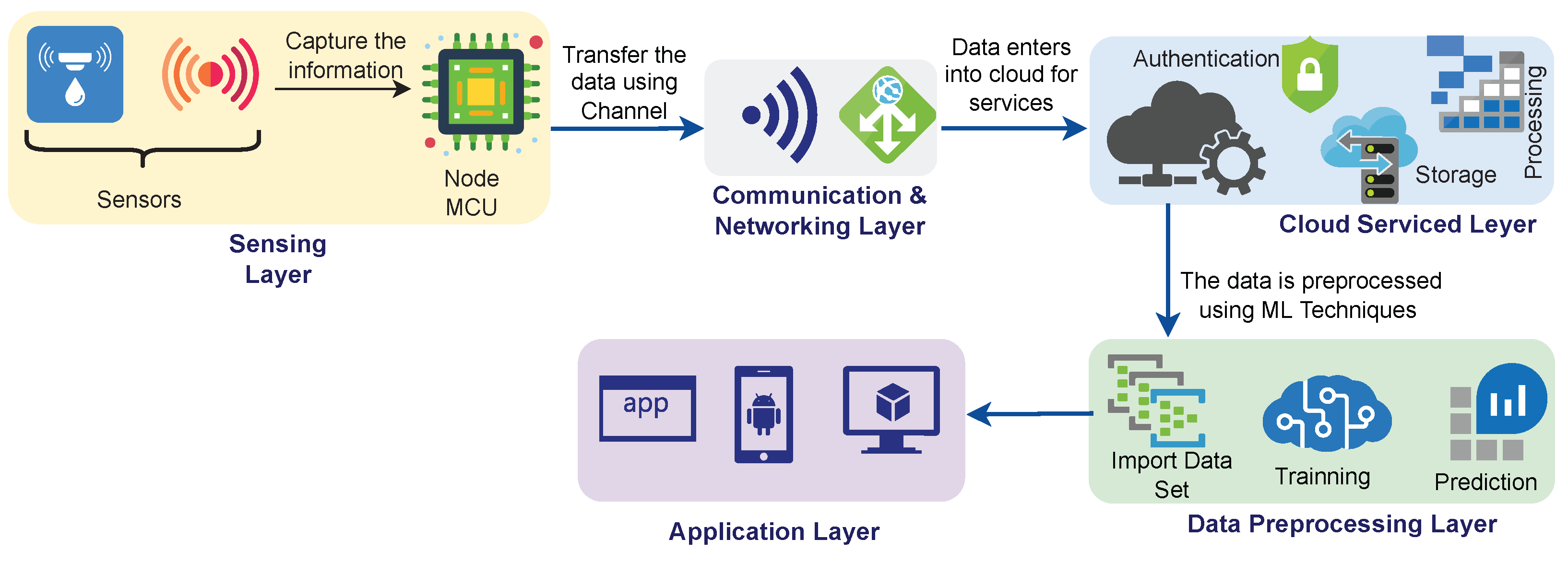
3.1. Layered Architecture of an IoT-Based Air-Quality Monitoring System for Agricultural Communities

Figure 2 represents the layered architecture of the IoT-based air-pollution monitoring system framework for the agricultural community. The layered architecture has been classified into five layers: a (i) sensing layer, (ii) communication and networking layer, (iii) cloud services layer, (iv) processing layer, and (v) application layer. The data collection was carried out between May 2019 and February 2020.

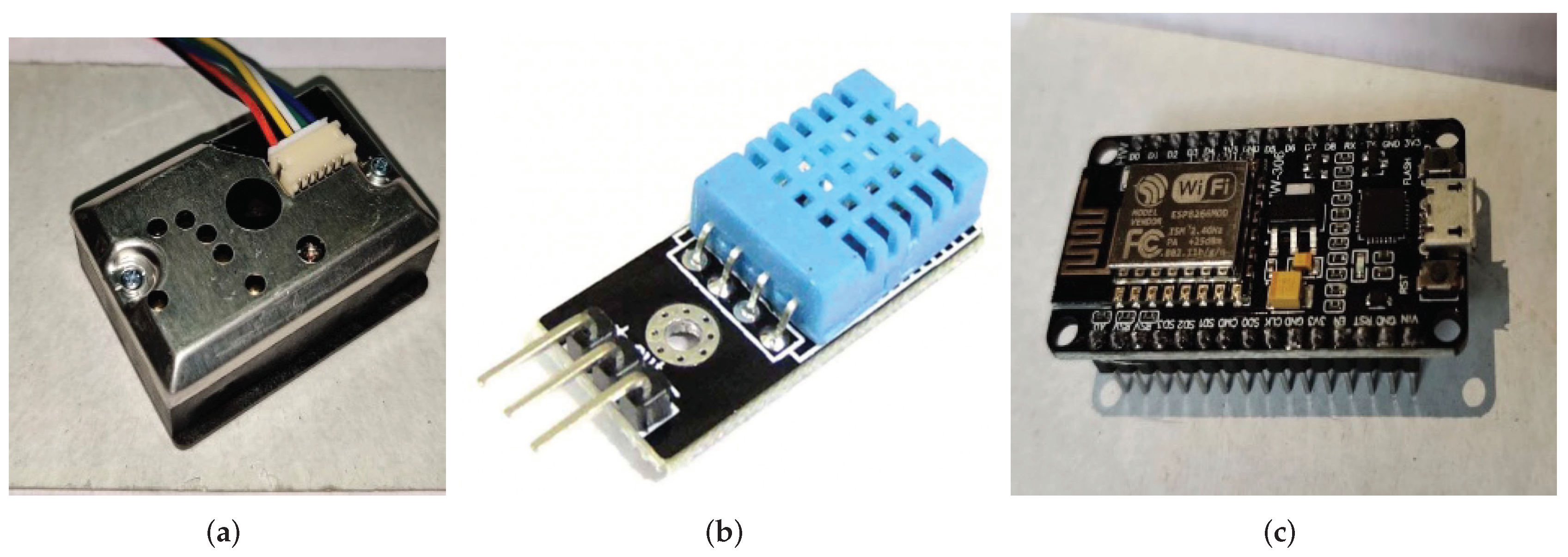
3.2. Physical Sensing Layer

The sensing layer contains a variety of sensing units such as a SDS021 Particulate Matter Sensor and DTH11 Temperature and Humidity Sensor. The SDS021 sensing unit can measure dust particles present in the surrounding environments such as PM${}_{2.5}$ and PM${}_{10}$. The DHT11 sensing unit can detect the temperature and humidity values of a particular location [74,75]. These sensing units are embedded with the NodeMCU(esp8266) micro-controller. These sensing units are placed to acquire the pollution-related updates of agricultural states and cities of India. Figure 3a–c, represents the design and experimental setup of IoT-based air-quality monitoring system for the agricultural community.

3.3. Communication and Networking Layer

The communication and networking layer is responsible for establishing a connection between a sensing layer, a cloud broker architecture (an MQTT broker), a pollution-data storage server, and a web interface. The Wi-Fi access point is essential for transmitting pollution data acquired by pollution sensing units via a cloud broker via the Internet.

3.4. Cloud Services Layer

The cloud services layer is responsible for storing various pollution data such as PM${}_{2.5}$, PM${}_{10}$, temperature, and humidity in the form of .csv files. This layer is also responsible for publishing the acquired air-quality data to the web interface via a cloud MQTT broker. This layer is also responsible for providing data privacy and security via third party SLAs (service level agreements) [76,77,78].

3.5. Processing Layer

The pollution-data processing layer analyses the received pollution data from various sensing units and generates different graphical results such as AQI analysis [79,80], PM${}_{2.5}$, and PM${}_{10}$ comparisons of India’s agragarian states and cities as described in Section 4.

Application Layer: the application layer provides real-time AQI monitoring updates of India’s agricultural states and cities via a GUI-based web interface.

The AQI is an essential and useful unitless color-coded index used by countries such as Europe, Canada, and Malaysia. The AQI metric is used worldwide to measure pollution conditions at a given point of time at a particular location (Source: http://www.wamis.org/agm/; accessed on 1 October 2020). The classification risk metric is employed in the conducted experiments to compute the AQI of a particular pollutant such as PM${}_{2.5}$ and PM${}_{10}$. As shown in

Table 2. A risk classification analysis of the Air Quality Index of India’s agrarian states (Source: https://www.epa.gov/sites/production/files/2014-05/documents/zell-aqi.pdf; accessed on 1 October 2020.

Risk Classification	AQI Values	Color-Coding
Good	0–50	Green
Moderate	51–100	Yellow
Unhealthy for Sensitive Groups	101–150	Orange
Unhealthy	151–200	Red
Very Unhealthy	201–300	Purple
Hazardous	300 and above	Brown

, the risk classification of pollution conditions is represented in various classification categories. Categorizes include good, moderate, unhealthy, very unhealthy, and hazardous. The Average AQI coefficient can be given by (Source: https://www.epa.gov/sites/production/files/2014-05/documents/zell-aqi.pdf; accessed on 1 October 2020 [81]).

$$\mathrm{AQI}\mathrm{coefficient}\mathrm{of}\mathrm{a}\mathrm{particular}\mathrm{pollutant}=\left[\frac{\left(AP{P}_{obs}-AP{P}_{min}\left(PAQ{L}_{max}-PAQ{I}_{min}\right)\right.}{POL{L}_{max}-POL{L}_{min}}\right]$$

(1)

where $AP{P}_{obs}$ = average measured concentration of a particular pollutant in 24 h in mg/m${}^3$, $AP{P}_{min}$ = the minimum concentration of an AQI of a particular pollutant calculated based on the risk classification metric, and $PAQ{I}_{min}$ = minimum AQI values of a specific pollutant calculated based on the risk classification metric. Where Pobs = average measured concentration in 24 h in mg/m${}^3$, $PAQ{I}_{max}$ = the maximum concentration of an AQI of a particular pollutant calculated based on the risk classification metric, $POL{L}_{min}$ = the minimum concentration of an AQI of a particular pollutant calculated based on the risk classification metric, and $POL{L}_{max}$ = the maximum concentration of an AQI of a particular pollutant calculated based on the risk classification metric. Section 3.1 discusses the detailed impacts of air pollution on yield crops. Section 3.2 presents India’s top polluted agrarian states’ in-depth investigation regarding AQI variations and PM${}_{2.5}$ and PM${}_{10}$ levels. Section 3.3 discusses the impact assessment of the AQI, PM${}_{2.5}$, and PM${}_{10}$ for India’s top cities affected by air pollution and its effects. The molecular conversion coefficient (MC) to convert a pollutant from ppb to $\mathsf{\mu }$g/m${}^3$ can be given by (Source: https://www.epa.gov/sites/production/files/2014-05/documents/zell-aqi.pdf; accessed on 10 December 2020),

$$\mathrm{CMC}\left(\mathsf{\mu }\mathrm{g}/{\mathrm{m}}^3\right)=\frac{\left[\right(ppb)\times mw]}{mv}$$

(2)

where $mw$ = molecular weight, and $mv$ = molecular volume. The molecular volume ($mv$) can be given by (Source: https://www.epa.gov/sites/production/files/2014-05/documents/zell-aqi.pdf; accessed on 10 December 2020),

$$mv\left(\mathrm{in}\mathrm{litres}\right)=\frac{[22.41\times T\times 1013]}{(273\times p)}$$

(3)

where T = temperature (K) and P = atmospheric pressure (hPa (hectopascal)).

4. Results and Discussions

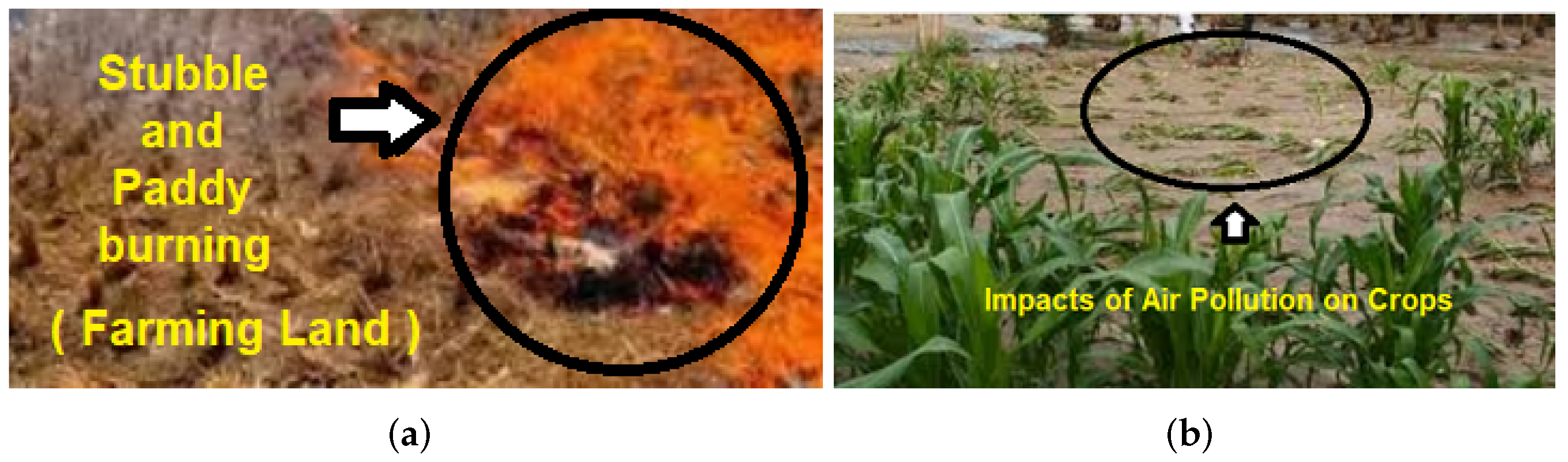
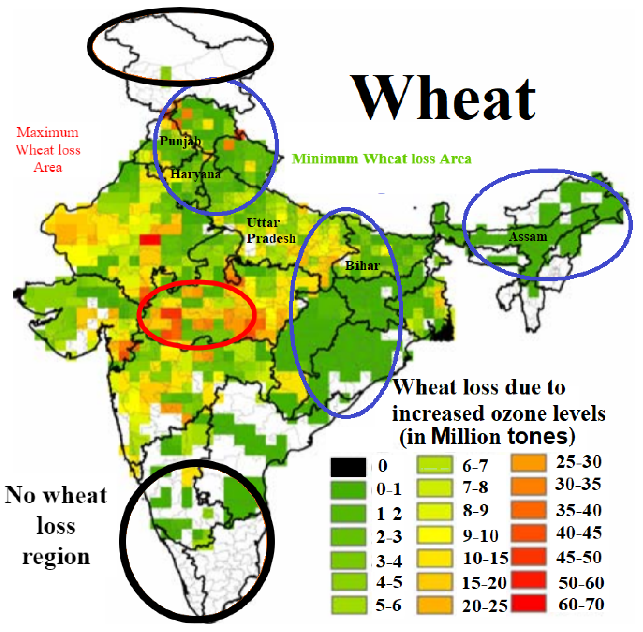
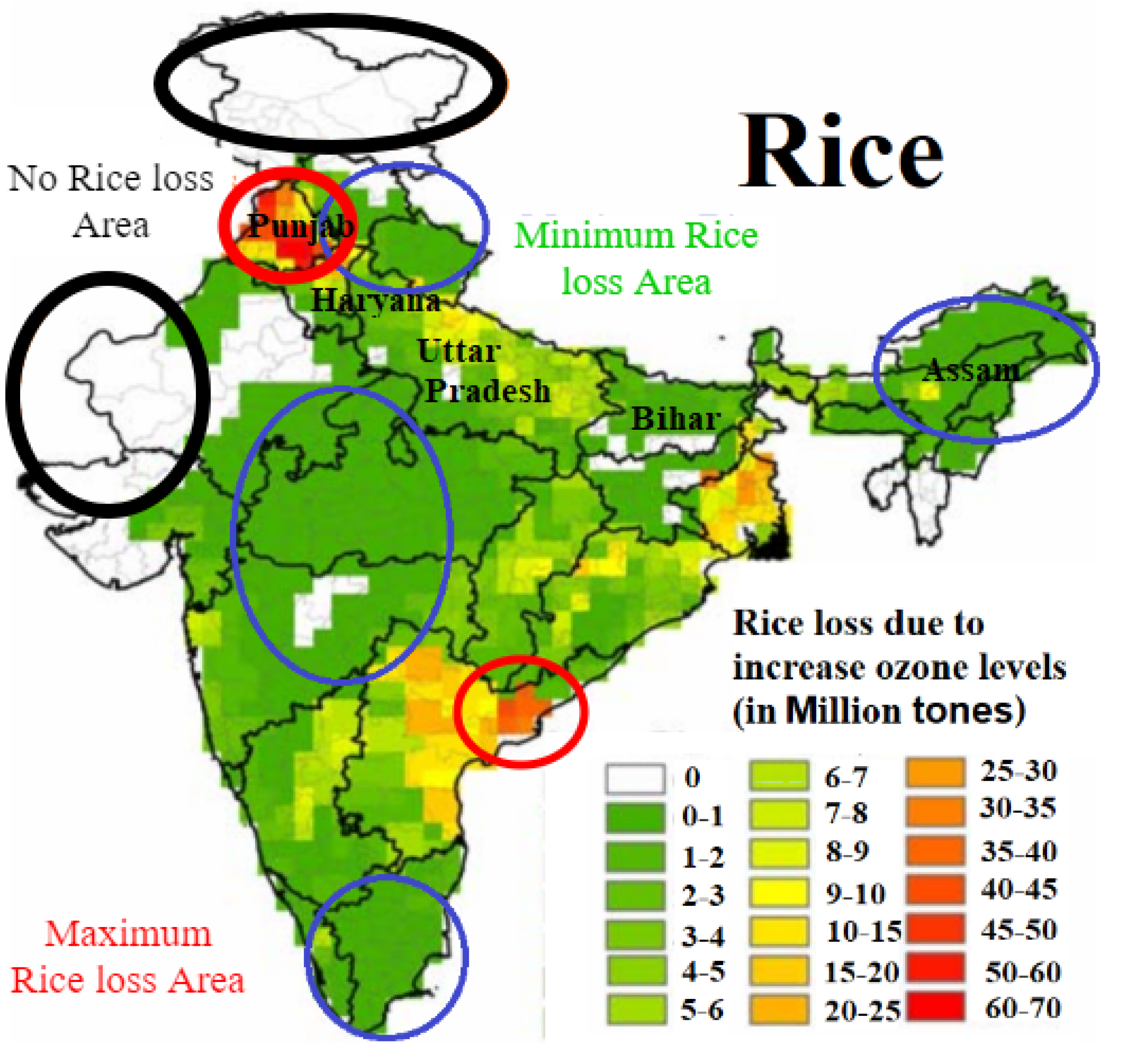
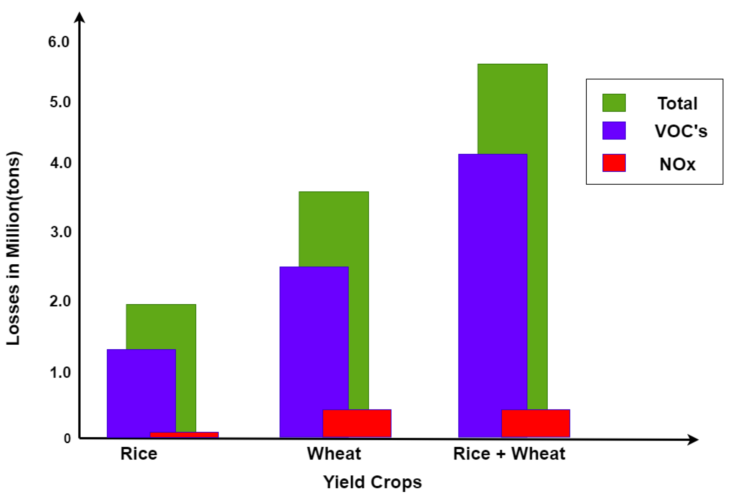
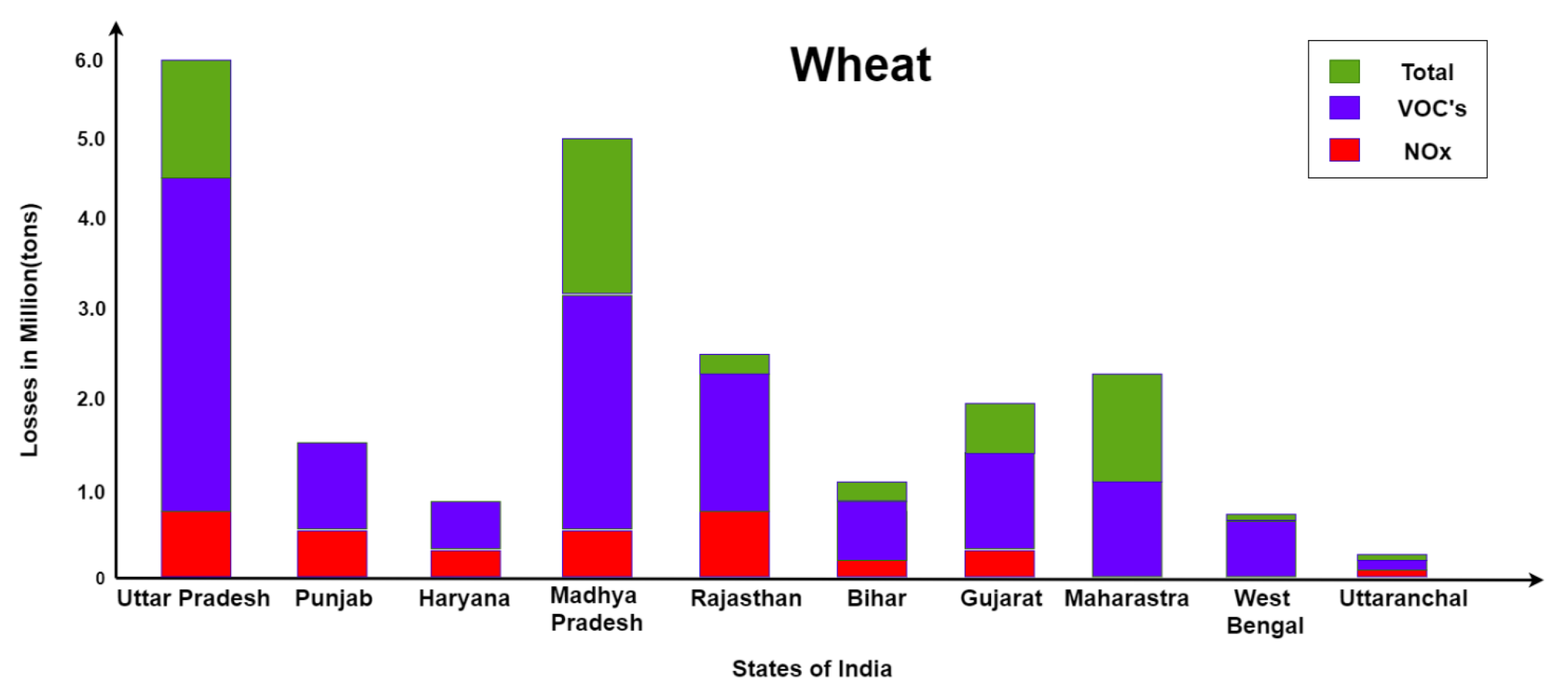
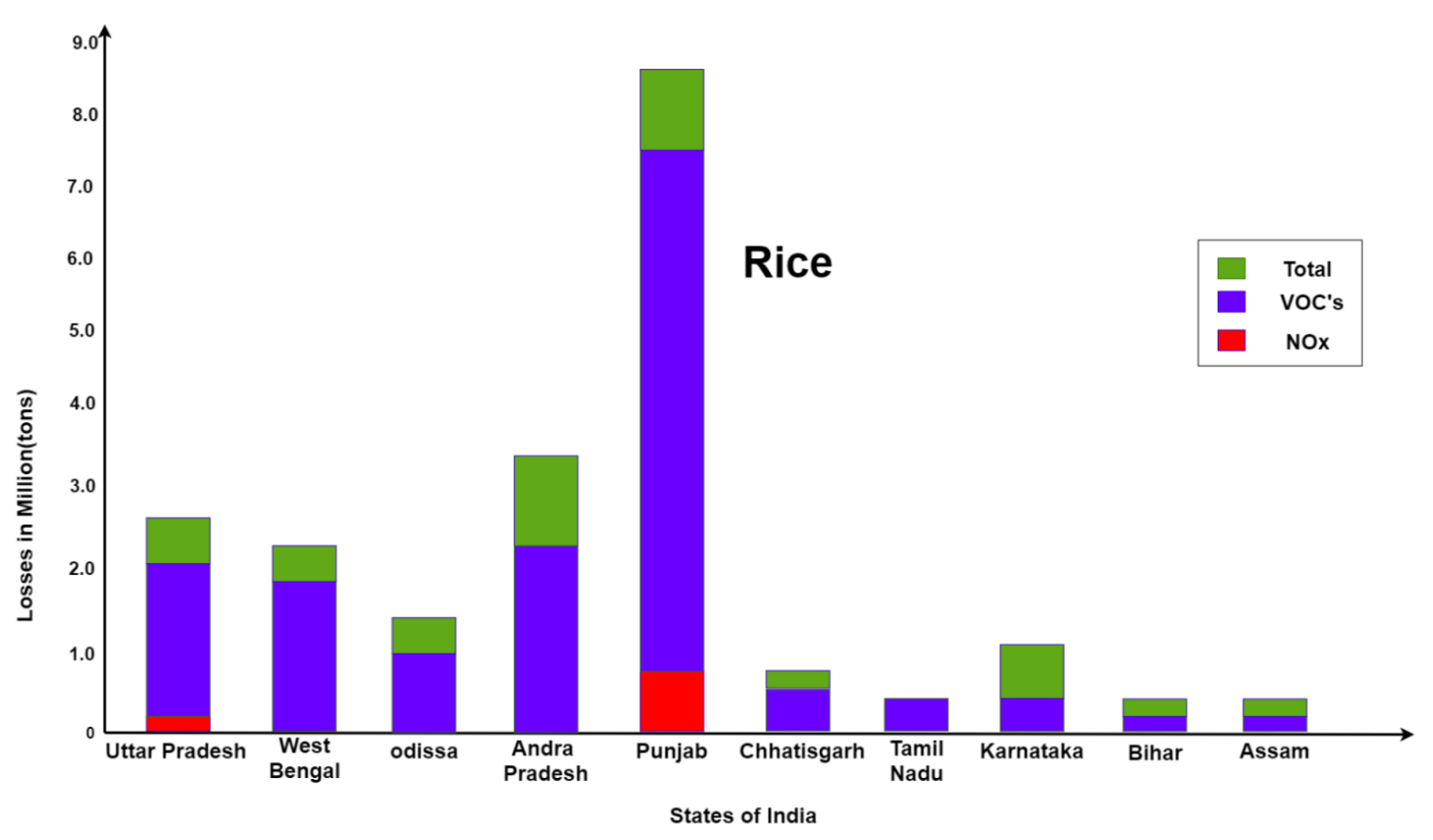
4.1. Impacts of Air Pollution on Yield Crops

Figure 4 represents the state-wise wheat loss (in million tons) in India due to increased ozone levels. It indicates a high wheat loss in crop-yielding states such as Rajasthan, Madhya Pradesh, Gujarat, and some regions of Himachal Pradesh. Variations in wheat loss are represented with red, yellow, green, and red colors on the scale of 0 to 70 million tons, as shown in Figure 4. The mass production of different types of crops throughout the year, in one place, increases the loss of crop yield, as well as increasing pollution due to its burning. Figure 5 represents the state-wise rice loss in India due to increased ozone levels. It also represents a significant wheat loss in Punjab, West Bengal, and Andhra Pradesh. Likewise, rice loss variations are represented with red, yellow, green, and white colors on the scale of 0 to 70 million tons, as shown in Figure 5.

Figure 6 compares the loss of rice and wheat produced in India in million tons. Due to this loss, the amount of VOCs generated is higher than the number of NOx gases generated. Variations in NOx such as nitric oxide (NO) and nitrogen dioxide (NO₂) and variation in volatile organic compounds (VOCs), and total are represented using red, blue, and green colors. Rice does not produce nitrogen oxide during its loss, wheat produces nitrogen-oxide variants, and when VOCs are mixed with nitrogen oxides in the air, they form smog. Totaling to almost 6 million tons of crop loss, the effects these practices and errors have on the climate and health conditions of people living nearby are immeasurable. Again, variations in NOx such as nitric oxide (NO) and nitrogen dioxide (NO₂) and variation in volatile organic compounds (VOCs) and total are represented using red, blue, and green colors.

A similar color scheme is applied to the rest of the figures. Figure 7 represents the state-wise wheat loss in India. Among all states, Uttar Pradesh tops the list with 0.6 million tons of wheat yield loss, followed by Madhya Pradesh, whereas Uttaranchal has achieved the bottom position with wheat loss of 0.040 million tons lost. Figure 8 represents the state-wise rice loss in India. Punjab has the most loss, with almost 0.9 million tons of rice yield lost, followed by Andhra Pradesh, whereas Tamil Nadu is the lowest, with approximately 0.020 million tons lost. It can be observed that Punjab faces a significant issue of rice burning, and, as mentioned previously, farmers in this region tend to burn significant amounts of rice to get the fields ready for the future wheat yield. While Punjab follows this trend the most, other states such as Andhra Pradesh, Uttar Pradesh, and West Bengal also face the same issues: mass-producing their crops on the same clock as Punjab.

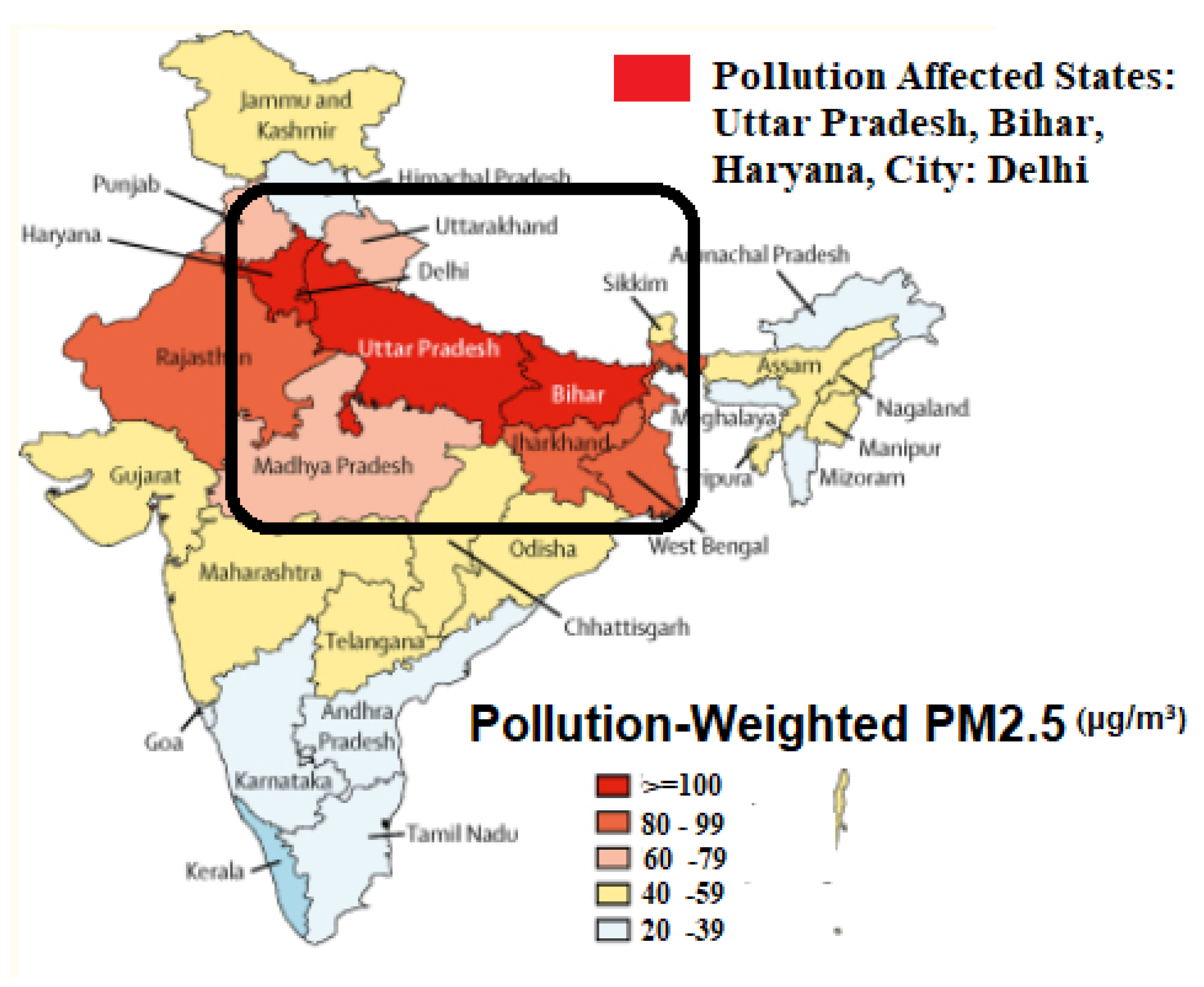
4.2. Air-Pollution Statistics (AQI) of Top Agrarian States of India

In this study, we used available pollution data provided by the Indian government on their official portal (www.aqi.in, accessed on 4 September 2022).

Table 3. An analysis of the AQI, PM${}_{2.5}$ ($\mathsf{\mu }$g/m${}^3$) and PM${}_{10}$ ($\mathsf{\mu }$g/m${}^3$) concentrations, temperature (°C), and humidity (%) in agrarian states of India (Source: www.aqui.in; accessed on 1 October 2020).

State	AQI	PM${}_{2.5}$ ($\mathsf{\mu }$g/m${}^3$)	PM${}_{10}$ ($\mathsf{\mu }$g/m${}^3$)	Temperature (°C)	Humidity (%)
Uttar Pradesh	249	240	145	34	80
Punjab	235	239	109	36	58
Haryana	235	227	122	32	74
Bihar	130	162	82	41	76
Assam	110	140	79	42	78

lists a statistical analysis of the AQI values of agrarian states in India. Based on this analysis, Uttar Pradesh and Punjab are the most and second-most polluted states of India with AQI values of 249 and 235. Haryana remains the third most polluted state of India, with an AQI of 235. This analysis also indicates that all agriculture-dominated states can be considered more polluted Indian states than non-agricultural states. Table 3 also compares the PM${}_{2.5}$ and PM${}_{10}$ indices, as well as the variations in temperature and humidity for agrarian states with the highest AQI indices. According to a source appointment survey by TERI (TERI Reports, 2018), 17% of the PM${}_{10}$ and 19% of the PM${}_{2.5}$ emissions in NCR Delhi derive from agricultural burning in nearby states Uttar Pradesh and Haryana. Therefore, agricultural burning in Delhi NCR has a 36% contribution to the total pollution, which is only based on PM${}_{2.5}$ and PM${}_{10}$ measurements.

Figure 9 represents a pollution map of India’s pollution-affected regions concerning PM${}_{2.5}$ levels. The most polluted agricultural states of India that exceed a hundred AQI index are represented by the red color. Figure 10a–c, depicts graphical analyses of the top three most polluted agrarian states of India between May 2019 and February 2020. Different colors are used for the following categories to represent the pollution impact analysis: (i) unhealthy for sensitive groups (orange), (ii) moderate (yellow), (iii) good (green), (iv) hazardous (dark pink), (v) very unhealthy (purple), and (vi) unhealthy (red). Based on the observations, seasonal changes have significantly impacted variations in the AQI. For Uttar Pradesh, we observe that AQI values have remained below the rudimentary level during autumn (September 2019 to January 2019). However, we also observe that the AQI has increased drastically in Uttar Pradesh, which is categorized as “unhealthy and very unhealthy” conditions during spring (February 2020 to May 2020) based on Indian weather conditions. This change’s primary reason is routine agricultural activities conducted by farmers, such as soil preparation, planting, and harvesting. These activities are at their peak during the spring. As part of this process, most farmers intentionally burn the remaining stubble (i.e., the components that remain after grain collection), such as wheat and paddies. Stubble burning has a severe impact on the surrounding environment and the farmers’ health. Similar practices are followed in agrarian states, such as Punjab and Haryana. This is also an alarming issue for urban cities adjacent to these agrarian states, such as Delhi, India’s capital. Recently, the inhabitants of Delhi have faced issues related to continuously degrading air quality. During the last year, Delhi’s AQI levels have exceeded 1000, which is unbearable for its civilians. Furthermore, in states such as Haryana and Punjab, AQI values have remained at peak values from December 2019 to April 2020. The AQI values have also increased significantly in the last several years. Air pollution has significantly affected the agricultural community and agrarian states, especially farmers, due to air-pollution-related health and environmental issues.

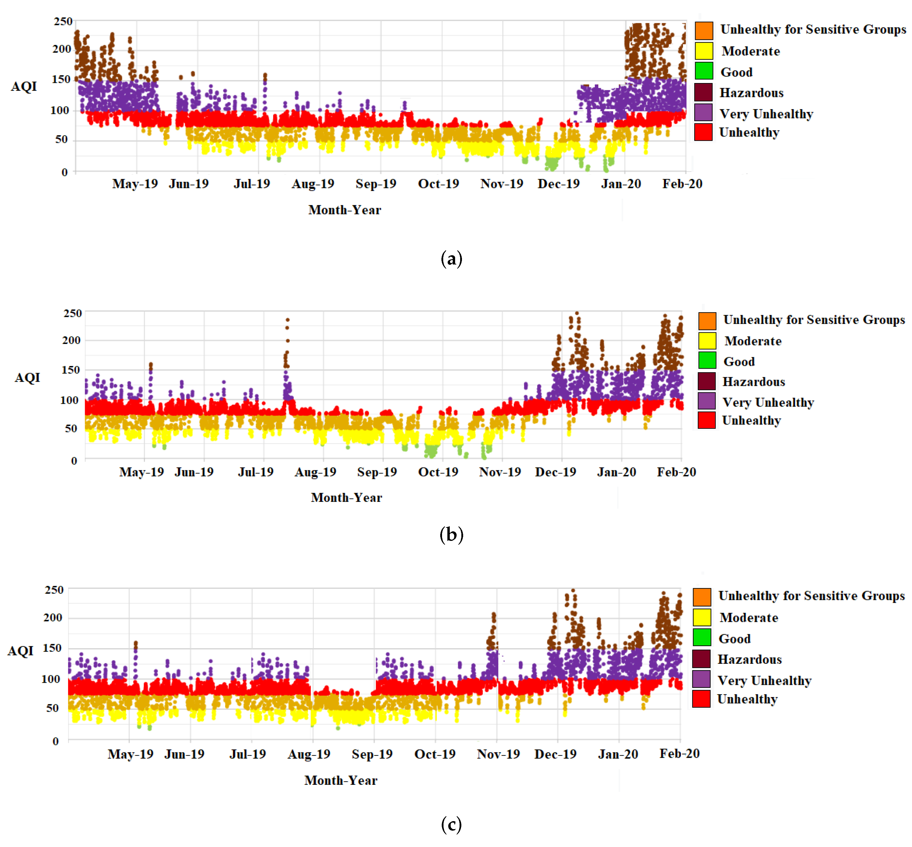
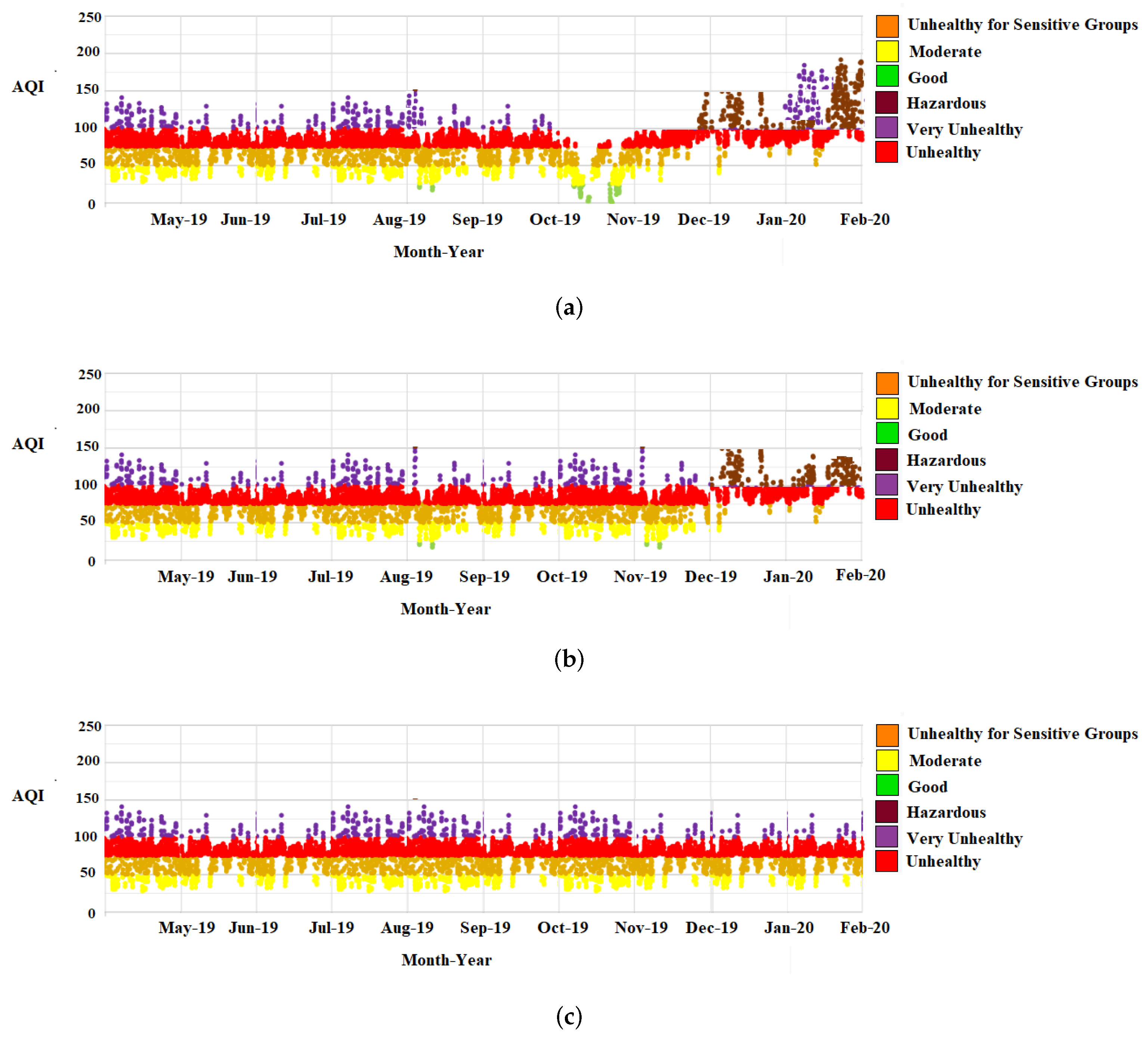
4.3. Analysis of Air-Pollution Affected Cities of India

We presented the pollution risk classification analysis of the agrarian pollution-affected Indian cities concerning the AQI values and PM${}_{2.5}$ and PM${}_{10}$ concentration.

Table 4. A city-wise analysis of the AQI, PM${}_{2.5}$ ($\mathsf{\mu }$g/m${}^3$) and PM${}_{10}$ ($\mathsf{\mu }$g/m${}^3$) concentrations, temperature (°C), and humidity (%) (Source: www.aqui.in; accessed on 1 October 2020).

City	AQI	PM${}_{2.5}$ ($\mathsf{\mu }$g/m${}^3$)	PM${}_{10}$ ($\mathsf{\mu }$g/m${}^3$)	Temperature (°C)	Humidity (%)
Delhi	159	81	94	23	61
Ghaziabad	125	78	86	36	58
Meerut	120	57	58	32	74

provides a real-time AQI analysis of these cities based on available pollution data (i.e., the www.aqi.in, accessed on 4 September 2022). This analysis also indicates that Delhi has achieved the premier position due to massive air-pollution impacts in recent years. Furthermore, Ghaziabad and Meerut are recently characterized by AQI values above 100. Table 4 also describes the impact analysis of the agrarian Indian cities concerning the PM${}_{2.5}$ and PM${}_{10}$ concentrations and the variations in temperature and humidity levels, where the highest PM${}_{2.5}$ and PM${}_{10}$ concentrations occurred in India’s capital city. As discussed previously, one of the primary reasons for these high values and concentrations is the burning of stubble and paddies in adjacent agriculture states, such as Haryana and Uttar Pradesh. Figure 11a–c presents an AQI seasonal analysis of the top most polluted cities of India between May 2019 and February 2020. Again, we used the same pollution risk metric classification analysis with six categories and colored graphical representations used previously for India’s agrarian states. Based on our observations, we find that seasonal changes have significantly impacted AQI variations in India’s top cities. As discussed previously, Delhi has remained the most polluted city of India, which has frequently faced challenging situations, such as low air quality and high PM${}_{2.5}$, PM${}_{10}$, and AQI levels. In January 2020, officials recorded an alarming pollution situation with high pollution levels in more than 90% of Delhi’s areas. All the schools and colleges were completely shut down for nearly a month due to air-pollution-related issues. Delhi’s pollution levels, Ghaziabad and Meerut, can be categorized as “very unhealthy” and “unhealthy” from 2019–2020.

5. Conclusions and Future Enhancements

Air pollution has become an important issue of the 21st century and significantly contributed to fatalities, especially in agricultural communities living in developing countries, such as India. Our analysis’s unique feature is the color-coding-based AQI risk-metric classification of the impacts of air pollution on India’s agrarian states and cities. We analyzed India’s most polluted agrarian states and cities in terms of AQI variations and PM${}_{2.5}$, and PM${}_{10}$ concentrations. The empirical study of the seasonal impacts of air pollution on the agrarian states and cities was presented for May 2019 to February 2020. Based on our results, we obtained several significant observations:

• Higher AQI, PM${}_{2.5}$, and PM${}_{10}$ levels were found in agriculturally dominated states such as Uttar Pradesh, Punjab, and Haryana.
• Among all the cities, India’s capital is the most polluted city and has faced significant challenges, such that it may experience alarming pollution levels in the future.
• The average AQI values fluctuate in various areas of the cities such as Delhi, where the AQI value in certain regions can vary by more than 500 on the AQI index. In the end, recent impacts of air pollution concerning AQI variations for May 2019 to February 2020, seasonal AQI variations, impacts of PM${}_{2.5}$ and PM${}_{10}$ in various agrarian states and Indian cities are presented using various color-coding-based graphical and tabular representations.

In the future, scientists may conduct extensive analyses of the impacts that air pollution has on critical resources, such as water and soil, and these scientists can investigate air pollution’s global, country, state, and city impacts.

References

1. Chakrabarti, S.; Khan, M.T.; Kishore, A.; Roy, D.; Scott, S.P. Risk of acute respiratory infection from crop burning in India: Estimating disease burden and economic welfare from satellite and national health survey data for 250,000 persons. Int. J. Epidemiol. 2019, 48, 1113–1124. [Google Scholar] [CrossRef] [PubMed] [Green Version]
2. Sanderfoot, O.V.; Holloway, T. Air pollution impacts on avian species via inhalation exposure and associated outcomes. Environ. Res. Lett. 2017, 12, 083002. [Google Scholar] [CrossRef]
3. Dedeurwaerdere, T. Global microbial commons: Institutional challenges for the global exchange and distribution of microorganisms in the life sciences. Res. Microbiol. 2010, 161, 414–421. [Google Scholar] [CrossRef] [PubMed]
4. Kularatna, N.; Sudantha, B. An environmental air pollution monitoring system based on the IEEE 1451 standard for low cost requirements. IEEE Sens. J. 2008, 8, 415–422. [Google Scholar] [CrossRef]
5. Kumar, S.; Sharma, D.; Singh, D.; Biswas, H.; Praveen, K.; Sharma, V. Estimating loss of ecosystem services due to paddy straw burning in North-west India. Int. J. Agric. Sustain. 2019, 17, 146–157. [Google Scholar] [CrossRef]
6. Scholz, R.W.; Wellmer, F.W. Losses and use efficiencies along the phosphorus cycle. Part 1: Dilemmata and losses in the mines and other nodes of the supply chain. Resour. Conserv. Recycl. 2015, 105, 216–234. [Google Scholar] [CrossRef]
7. Devarakonda, S.; Sevusu, P.; Liu, H.; Liu, R.; Iftode, L.; Nath, B. Real-time air quality monitoring through mobile sensing in metropolitan areas. In Proceedings of the 2nd ACM SIGKDD International Workshop on Urban Computing, Chicago, IL, USA, 11 August 2013; pp. 1–8. [Google Scholar]
8. Zhang, L.; Yan, C.; Guo, Q.; Zhang, J.; Ruiz-Menjivar, J. The impact of agricultural chemical inputs on environment: Global evidence from informetrics analysis and visualization. Int. J. Low-Carbon Technol. 2018, 13, 338–352. [Google Scholar] [CrossRef] [Green Version]
9. Gadekallu, T.R.; Rajput, D.S.; Reddy, M.; Lakshmanna, K.; Bhattacharya, S.; Singh, S.; Jolfaei, A.; Alazab, M. A novel PCA—Whale optimization-based deep neural network model for classification of tomato plant diseases using GPU. J. Real-Time Image Process. 2021, 18, 1383–1396. [Google Scholar] [CrossRef]
10. Deepa, N.; Khan, M.Z.; Prabadevi, B.; PM, D.R.V.; Maddikunta, P.K.R.; Gadekallu, T.R. Multiclass model for agriculture development using multivariate statistical method. IEEE Access 2020, 8, 183749–183758. [Google Scholar] [CrossRef]
11. Chaganti, R.; Varadarajan, V.; Gorantla, V.S.; Gadekallu, T.R.; Ravi, V. Blockchain-Based Cloud-Enabled Security Monitoring Using Internet of Things in Smart Agriculture. Future Internet 2022, 14, 250. [Google Scholar] [CrossRef]
12. Aneja, V.P.; Schlesinger, W.H.; Erisman, J.W. Effects of Agriculture upon the Air Quality and Climate: Research, Policy, and Regulations; ACS Publications: Washington, DC, USA, 2009. [Google Scholar]
13. Burney, J.; Ramanathan, V. Recent climate and air pollution impacts on Indian agriculture. Proc. Natl. Acad. Sci. USA 2014, 111, 16319–16324. [Google Scholar] [CrossRef] [Green Version]
14. Harizanova-Bartos, H.; Stoyanova, Z. Impact of agriculture on air pollution. CBU Int. Conf. Proc. 2018, 6, 1071–1076. [Google Scholar] [CrossRef] [Green Version]
15. Hang, Y.; Wang, Q.; Zhou, D.; Zhang, L. Factors influencing the progress in decoupling economic growth from carbon dioxide emissions in China’s manufacturing industry. Resour. Conserv. Recycl. 2019, 146, 77–88. [Google Scholar] [CrossRef]
16. Breunig, H.M.; Huntington, T.; Jin, L.; Robinson, A.; Scown, C.D. Temporal and geographic drivers of biomass residues in California. Resour. Conserv. Recycl. 2018, 139, 287–297. [Google Scholar] [CrossRef]
17. Cruz, N.C.; Silva, F.C.; Tarelho, L.A.; Rodrigues, S.M. Critical review of key variables affecting potential recycling applications of ash produced at large-scale biomass combustion plants. Resour. Conserv. Recycl. 2019, 150, 104427. [Google Scholar] [CrossRef]
18. Shen, F.; Ge, X.; Hu, J.; Nie, D.; Tian, L.; Chen, M. Air pollution characteristics and health risks in Henan Province, China. Environ. Res. 2017, 156, 625–634. [Google Scholar] [CrossRef] [PubMed]
19. Shaibu-Imodagbe, E. The impact of some specific air pollutants on agricultural productivity. Environmentalist 1991, 11, 33–38. [Google Scholar] [CrossRef]
20. Zhang, C.; Liu, S.; Wu, S.; Jin, S.; Reis, S.; Liu, H.; Gu, B. Rebuilding the linkage between livestock and cropland to mitigate agricultural pollution in China. Resour. Conserv. Recycl. 2019, 144, 65–73. [Google Scholar] [CrossRef]
21. Beig, G. Impact of Air Pollution on Agriculture; Indian Institute of Tropical Meteorology, Ministry of Earth Sciences: Pune, India, 2014. [Google Scholar]
22. Salamone, F.; Belussi, L.; Danza, L.; Galanos, T.; Ghellere, M.; Meroni, I. Design and development of a nearable wireless system to control indoor air quality and indoor lighting quality. Sensors 2017, 17, 1021. [Google Scholar] [CrossRef] [PubMed]
23. Zhang, T.; Yang, Y.; Ni, J.; Xie, D. Adoption behavior of cleaner production techniques to control agricultural non-point source pollution: A case study in the Three Gorges Reservoir Area. J. Clean. Prod. 2019, 223, 897–906. [Google Scholar] [CrossRef]
24. Lu, W.; Wang, M.; Wu, J.; Jiang, Q.; Jin, J.; Jin, Q.; Yang, W.; Chen, J.; Wang, Y.; Xiao, M. Spread of chloramphenicol and tetracycline resistance genes by plasmid mobilization in agricultural soil. Environ. Pollut. 2020, 260, 113998. [Google Scholar] [CrossRef]
25. Douterelo, I.; Perona, E.; Mateo, P. Use of cyanobacteria to assess water quality in running waters. Environ. Pollut. 2004, 127, 377–384. [Google Scholar] [CrossRef]
26. Zhu, G.B.; Singh, B.; Zhu, Y.G. Anaerobic ammonium oxidation in agricultural soils-synthesis and prospective. Environ. Pollut. 2019, 244, 127–134. [Google Scholar]
27. Cox, L.A., Jr. Communicating more clearly about deaths caused by air pollution. In Quantitative Risk Analysis of Air Pollution Health Effects; Springer: Berlin/Heidelberg, Germany, 2021; pp. 525–540. [Google Scholar]
28. Cox, L.A., Jr. Should health risks of air pollution be studied scientifically? Glob. Epidemiol. 2019, 1, 100015. [Google Scholar] [CrossRef]
29. LaKind, J.S.; Burns, C.J.; Erickson, H.; Graham, S.E.; Jenkins, S.; Johnson, G.T. Bridging the epidemiology risk assessment gap: An NO2 case study of the Matrix. Glob. Epidemiol. 2020, 2, 100017. [Google Scholar] [CrossRef]
30. Goodman, J.E.; Prueitt, R.L.; Harbison, R.D.; Johnson, G.T. Systematically evaluating and integrating evidence in National Ambient Air Quality Standards reviews. Glob. Epidemiol. 2020, 2, 100019. [Google Scholar] [CrossRef]
31. Lu, C.; Hong, Y.; Liu, J.; Gao, Y.; Ma, Z.; Yang, B.; Ling, W.; Waigi, M.G. A PAH-degrading bacterial community enriched with contaminated agricultural soil and its utility for microbial bioremediation. Environ. Pollut. 2019, 251, 773–782. [Google Scholar] [CrossRef]
32. Chakraborty, P.; Zhang, G.; Li, J.; Sivakumar, A.; Jones, K.C. Occurrence and sources of selected organochlorine pesticides in the soil of seven major Indian cities: Assessment of air–soil exchange. Environ. Pollut. 2015, 204, 74–80. [Google Scholar] [CrossRef]
33. Anwar, A.; Ayub, M.; Khan, N.; Flahault, A. Nexus between air pollution and neonatal deaths: A case of Asian countries. Int. J. Environ. Res. Public Health 2019, 16, 4148. [Google Scholar] [CrossRef] [Green Version]
34. Cassou, E.; Jaffee, S.M.; Ru, J. The Challenge of Agricultural Pollution: Evidence from China, Vietnam, and the Philippines; World Bank Publications: Herndon, VA, USA, 2018. [Google Scholar]
35. Liang, C.; Xiao, H.; Hu, Z.; Zhang, X.; Hu, J. Uptake, transportation, and accumulation of C60 fullerene and heavy metal ions (Cd, Cu, and Pb) in rice plants grown in an agricultural soil. Environ. Pollut. 2018, 235, 330–338. [Google Scholar] [CrossRef]
36. Badura, M.; Batog, P.; Drzeniecka-Osiadacz, A.; Modzel, P. Evaluation of low-cost sensors for ambient PM2.5 monitoring. J. Sens. 2018, 2018, 5096540. [Google Scholar] [CrossRef]
37. Kim, J.; Hwangbo, H. Sensor-based optimization model for air quality improvement in home IoT. Sensors 2018, 18, 959. [Google Scholar] [CrossRef] [Green Version]
38. Mad Saad, S.; Andrew, A.M.; Md Shakaff, A.Y.; Mat Dzahir, M.A.; Hussein, M.; Mohamad, M.; Ahmad, Z.A. Pollutant recognition based on supervised machine learning for indoor air quality monitoring systems. Appl. Sci. 2017, 7, 823. [Google Scholar] [CrossRef]
39. Abbasi, A.; Sajid, A.; Haq, N.; Rahman, S.; Misbah, Z.t.; Sanober, G.; Ashraf, M.; Kazi, A.G. Agricultural pollution: An emerging issue. In Improvement of Crops in the Era of Climatic Changes; Springer: Berlin/Heidelberg, Germany, 2014; pp. 347–387. [Google Scholar]
40. Sinclair, M.; Zhang, Y.; Descovich, K.; Phillips, C.J. Farm animal welfare science in China—A bibliometric review of Chinese literature. Animals 2020, 10, 540. [Google Scholar] [CrossRef] [Green Version]
41. Fatmi, Z.; Ntani, G.; Coggon, D. Levels and determinants of fine particulate matter and carbon monoxide in kitchens using biomass and non-biomass fuel for cooking. Int. J. Environ. Res. Public Health 2020, 17, 1287. [Google Scholar] [CrossRef] [Green Version]
42. Truzzi, C.; Annibaldi, A.; Girolametti, F.; Giovannini, L.; Riolo, P.; Ruschioni, S.; Olivotto, I.; Illuminati, S. A chemically safe way to produce insect biomass for possible application in feed and food production. Int. J. Environ. Res. Public Health 2020, 17, 2121. [Google Scholar] [CrossRef] [Green Version]
43. Vicedo-Cabrera, A.; Sera, F.; Liu, C.; Armstrong, B.; Milojevic, A.; Guo, Y.; Tong, S.; Lavigne, E.; Kyselỳ, J.; Urban, A.; et al. Short term association between ozone and mortality: Global two stage time series study in 406 locations in 20 countries. BMJ 2020, 368, m108. [Google Scholar] [CrossRef] [Green Version]
44. Quiros, R.; Sanchez, A.; Font, X.; Artola, A. New Biodegradable Waste Management Plans Proposed and Evaluated. Sci. Environ. Policy 2015, 411. Available online: https://portalrecerca.uab.cat/en/publications/new-biodegradable-waste-management-plans-proposed-and-evaluated (accessed on 4 September 2022).
45. North, D.W. Commentary on “Should health risks of air pollution be studied scientifically?” by Louis Anthony Cox, Jr. Glob. Epidemiol. 2020, 2, 100021. [Google Scholar] [CrossRef]
46. Kim, J.; Kim, M.; Choi, M. Air Pollution in Eastern Asia: An Integrated Perspective. Air Pollut. East. Asia Integr. Perspect. 2017, 16, 323–333. [Google Scholar]
47. Chen, R.; Kan, H.; Chen, B.; Huang, W.; Bai, Z.; Song, G.; Pan, G. Association of particulate air pollution with daily mortality: The China Air Pollution and Health Effects Study. Am. J. Epidemiol. 2012, 175, 1173–1181. [Google Scholar] [CrossRef] [Green Version]
48. Chen, R.; Zhang, Y.; Yang, C.; Zhao, Z.; Xu, X.; Kan, H. Acute effect of ambient air pollution on stroke mortality in the China air pollution and health effects study. Stroke 2013, 44, 954–960. [Google Scholar] [CrossRef] [Green Version]
49. Christidis, T.; Erickson, A.C.; Pappin, A.J.; Crouse, D.L.; Pinault, L.L.; Weichenthal, S.A.; Brook, J.R.; van Donkelaar, A.; Hystad, P.; Martin, R.V.; et al. Low concentrations of fine particle air pollution and mortality in the Canadian Community Health Survey cohort. Environ. Health 2019, 18, 1–16. [Google Scholar] [CrossRef]
50. Li, M.; Wang, W.; Wang, Z.; Xue, Y. Prediction of PM2.5 concentration based on the similarity in air quality monitoring network. Build. Environ. 2018, 137, 11–17. [Google Scholar]
51. Amsalu, E.; Wang, T.; Li, H.; Liu, Y.; Wang, A.; Liu, X.; Tao, L.; Luo, Y.; Zhang, F.; Yang, X.; et al. Acute effects of fine particulate matter (PM2.5) on hospital admissions for cardiovascular disease in Beijing, China: A time-series study. Environ. Health 2019, 18, 70. [Google Scholar] [CrossRef] [Green Version]
52. Lasko, K.; Vadrevu, K. Improved rice residue burning emissions estimates: Accounting for practice-specific emission factors in air pollution assessments of Vietnam. Environ. Pollut. 2018, 236, 795–806. [Google Scholar] [CrossRef]
53. Augusto, S.; Máguas, C.; Matos, J.; Pereira, M.J.; Branquinho, C. Lichens as an integrating tool for monitoring PAH atmospheric deposition: A comparison with soil, air and pine needles. Environ. Pollut. 2010, 158, 483–489. [Google Scholar] [CrossRef]
54. Beckett, K.P.; Freer-Smith, P.; Taylor, G. Urban woodlands: Their role in reducing the effects of particulate pollution. Environ. Pollut. 1998, 99, 347–360. [Google Scholar] [CrossRef]
55. Pani, S.K.; Wang, S.H.; Lin, N.H.; Chantara, S.; Lee, C.T.; Thepnuan, D. Black carbon over an urban atmosphere in northern peninsular Southeast Asia: Characteristics, source apportionment, and associated health risks. Environ. Pollut. 2020, 259, 113871. [Google Scholar] [CrossRef]
56. Rico, A.; Oliveira, R.; McDonough, S.; Matser, A.; Khatikarn, J.; Satapornvanit, K.; Nogueira, A.J.; Soares, A.M.; Domingues, I.; Van den Brink, P.J. Use, fate and ecological risks of antibiotics applied in tilapia cage farming in Thailand. Environ. Pollut. 2014, 191, 8–16. [Google Scholar] [CrossRef]
57. Zanobetti, A.; Schwartz, J. Mortality displacement in the association of ozone with mortality: An analysis of 48 cities in the United States. Am. J. Respir. Crit. Care Med. 2008, 177, 184–189. [Google Scholar] [CrossRef] [PubMed]
58. Brown, P.; Maher, Y.I.; Balakrishnan, K.; Fu, S.H.; Kumar, R.; Chakma, J.; Menon, G.; Dikshit, R.; Dhaliwal, R.; Rodriguez, P.S.; et al. Mortality from Particulate Matter 2.5 in India: National Prospective Proportional Mortality Study. 2019. Available online: https://papers.ssrn.com/sol3/papers.cfm?abstract_id=3468394 (accessed on 4 September 2022).
59. Huang, S.; Xiong, J.; Vieira, C.L.; Blomberg, A.J.; Gold, D.R.; Coull, B.A.; Sarosiek, K.; Schwartz, J.D.; Wolfson, J.M.; Li, J.; et al. Short-term exposure to ambient particle gamma radioactivity is associated with increased risk for all-cause non-accidental and cardiovascular mortality. Sci. Total Environ. 2020, 721, 137793. [Google Scholar] [CrossRef] [PubMed]
60. Huang, J.; Duan, N.; Ji, P.; Ma, C.; Ding, Y.; Yu, Y.; Zhou, Q.; Sun, W. A crowdsource-based sensing system for monitoring fine-grained air quality in urban environments. IEEE Internet Things J. 2018, 6, 3240–3247. [Google Scholar] [CrossRef]
61. Swaminathan, M. Bio-diversity: An effective safety net against environmental pollution. Environ. Pollut. 2003, 126, 287–291. [Google Scholar] [CrossRef]
62. Agudelo-Castañeda, D.M.; Teixeira, E.C.; Schneider, I.L.; Lara, S.R.; Silva, L.F. Exposure to polycyclic aromatic hydrocarbons in atmospheric PM1.0 of urban environments: Carcinogenic and mutagenic respiratory health risk by age groups. Environ. Pollut. 2017, 224, 158–170. [Google Scholar] [CrossRef]
63. Mills, M.C.; Lee, J. The threat of carbapenem-resistant bacteria in the environment: Evidence of widespread contamination of reservoirs at a global scale. Environ. Pollut. 2019, 255, 113143. [Google Scholar] [CrossRef] [PubMed]
64. Al-Haija, Q.A.; Al-Qadeeb, H.; Al-Lwaimi, A. Case Study: Monitoring of AIR quality in King Faisal University using a microcontroller and WSN. Procedia Comput. Sci. 2013, 21, 517–521. [Google Scholar] [CrossRef] [Green Version]
65. Al-Ali, A.; Zualkernan, I.; Aloul, F. A mobile GPRS-sensors array for air pollution monitoring. IEEE Sens. J. 2010, 10, 1666–1671. [Google Scholar] [CrossRef]
66. Li, J.; Li, M.; Xin, J.; Lai, B.; Ma, Q. Wireless sensor network for indoor air quality monitoring. Sens. Transducers 2014, 172, 86. [Google Scholar]
67. Kumar, A.; Hancke, G.P. Energy efficient environment monitoring system based on the IEEE 802.15.4 standard for low cost requirements. IEEE Sens. J. 2014, 14, 2557–2566. [Google Scholar] [CrossRef] [Green Version]
68. Ferdoush, S.; Li, X. Wireless sensor network system design using Raspberry Pi and Arduino for environmental monitoring applications. Procedia Comput. Sci. 2014, 34, 103–110. [Google Scholar] [CrossRef] [Green Version]
69. Bacco, M.; Delmastro, F.; Ferro, E.; Gotta, A. Environmental monitoring for smart cities. IEEE Sens. J. 2017, 17, 7767–7774. [Google Scholar] [CrossRef]
70. Tiwari, A.; Sadistap, S.; Mahajan, S. Development of environment monitoring system using internet of things. In Ambient Communications and Computer Systems; Springer: Berlin/Heidelberg, Germany, 2018; pp. 403–412. [Google Scholar]
71. Marques, G.; Pires, I.M.; Miranda, N.; Pitarma, R. Air quality monitoring using assistive robots for ambient assisted living and enhanced living environments through internet of things. Electronics 2019, 8, 1375. [Google Scholar] [CrossRef] [Green Version]
72. Dhingra, S.; Madda, R.B.; Gandomi, A.H.; Patan, R.; Daneshmand, M. Internet of Things mobile–air pollution monitoring system (IoT-Mobair). IEEE Internet Things J. 2019, 6, 5577–5584. [Google Scholar] [CrossRef]
73. Sun, Z.; Zhu, D. Exposure to outdoor air pollution and its human health outcomes: A scoping review. PLoS ONE 2019, 14, e0216550. [Google Scholar] [CrossRef] [PubMed]
74. Maddikunta, P.K.R.; Hakak, S.; Alazab, M.; Bhattacharya, S.; Gadekallu, T.R.; Khan, W.Z.; Pham, Q.V. Unmanned aerial vehicles in smart agriculture: Applications, requirements, and challenges. IEEE Sens. J. 2021, 21, 17608–17619. [Google Scholar] [CrossRef]
75. Manikandan, S.; Kaliyaperumal, G.; Hakak, S.; Gadekallu, T.R. Curve-Aware Model Predictive Control (C-MPC) Trajectory Tracking for Automated Guided Vehicle (AGV) over On-Road, In-Door, and Agricultural-Land. Sustainability 2022, 14, 12021. [Google Scholar] [CrossRef]
76. Liyanage, M.; Ahmed, I.; Okwuibe, J.; Ylianttila, M.; Kabir, H.; Santos, J.L.; Kantola, R.; Perez, O.L.; Itzazelaia, M.U.; De Oca, E.M. Enhancing security of software defined mobile networks. IEEE Access 2017, 5, 9422–9438. [Google Scholar] [CrossRef]
77. He, D.; Zeadally, S.; Kumar, N.; Lee, J.H. Anonymous authentication for wireless body area networks with provable security. IEEE Syst. J. 2016, 11, 2590–2601. [Google Scholar] [CrossRef]
78. Feng, Q.; He, D.; Zeadally, S.; Khan, M.K.; Kumar, N. A survey on privacy protection in blockchain system. J. Netw. Comput. Appl. 2019, 126, 45–58. [Google Scholar] [CrossRef]
79. Gadekallu, T.; Kidwai, B.; Sharma, S.; Pareek, R.; Karnam, S. Application of data mining techniques in weather forecasting. In Sentiment Analysis and Knowledge Discovery in Contemporary Business; IGI Global: Hershey, PA, USA, 2019; pp. 162–174. [Google Scholar]
80. Li, X.; Tan, J.; Liu, A.; Vijayakumar, P.; Kumar, N.; Alazab, M. A novel UAV-enabled data collection scheme for intelligent transportation system through UAV speed control. IEEE Trans. Intell. Transp. Syst. 2020, 22, 2100–2110. [Google Scholar] [CrossRef]
81. Barot, V.; Kapadia, V.; Pandya, S. QoS enabled IoT based low cost air quality monitoring system with power consumption optimization. Cybern. Inf. Technol. 2020, 20, 122–140. [Google Scholar] [CrossRef]
Figure 1. The impacts of air pollution on (a) farming land, (b) crops.
Sustainability 14 13098 g001
Figure 2. Layered architecture of IoT-based air-quality monitoring system for agricultural community.
Sustainability 14 13098 g002
Figure 3. Design and experimental setup of IoT-based air-quality monitoring system for agricultural communities (a) SDS021 sensing unit, (b) DHT11 sensing unit, (c) NodeMCU(esp8266) microcontroller.
Sustainability 14 13098 g003
Figure 4. Wheat loss map of India (variations in wheat loss are represented with red, yellow, green, and white colors on the scale of 0 to 70 Million tons) (Source: http://www.wamis.org/agm/; accessed on 1 October 2020).
Sustainability 14 13098 g004
Figure 5. Rice loss map of India (variations in rice loss are represented with red, yellow, green, and white colors on the scale of 0 to 70 Million tons) (Source: http://www.wamis.org/agm/; accessed on 1 October 2020).
Sustainability 14 13098 g005
Figure 6. A bar-chart representation of comparison of rice and wheat loss of India concerning variation in NOx such as a nitric oxide (NO) and nitrogen dioxide (NO2) (in red color) and variation in volatile organic compounds (VOCs) (purple color), total (in green color) (Source: http://www.wamis.org/agm/; accessed on 1 October 2020).
Sustainability 14 13098 g006
Figure 7. State-wise wheat loss bar-chart representation of India concerning variations in NOx such as a nitric oxide (NO) and nitrogen dioxide (NO2) (in red color) and variation in volatile organic compounds (VOCs) (purple color), total (in green color) (Source: http://www.wamis.org/agm/; accessed on 1 October 2020).
Sustainability 14 13098 g007
Figure 8. A bar-chart representation of state-wise rice loss of India concerning variation in NOx such as a nitric oxide (NO) and dioxide (NO2) (in red color) and variation in volatile organic compounds (VOCs) (purple color), total (in green color) (Source: http://www.wamis.org/agm/; accessed on 1 October 2020).
Sustainability 14 13098 g008
Figure 9. A pollution analysis map of India’s affected regions (Source: www.aqui.in; accessed on 1 October 2020).
Sustainability 14 13098 g009
Figure 10. Air-pollution statistics (AQI) of top agrarian states of India (from May 2019 to February 2020) (a) Uttar Pradesh (b) Haryana, and (c) Punjab (Source: www.aqui.in; accessed on 1 October 2020).
Sustainability 14 13098 g010
Figure 11. Analysis of air-pollution-affected cities of India (from May 2019 to February 2020): (a) Delhi, (b) Ghaziabad, (c) Meerut (Source: www.aqui.in; accessed on 1 October 2020).
Sustainability 14 13098 g011