Article

Spatio-Temporal Impact of Global Migration on Carbon Transfers Based on Complex Network and Stepwise Regression Analysis

1
School of Environmental Science and Engineering, Shanghai Jiao Tong University, Shanghai 200240, China
2
Center for Energy Development and Environmental Protection, Jiangsu University, Zhenjiang 212013, China
3
School of Mathematics, Hunan University, Changsha 410082, China
4
School of Mechanical Engineering, Jiangsu University, Zhenjiang 212013, China
*
Author to whom correspondence should be addressed.
Sustainability 2022, 14(2), 844; https://doi.org/10.3390/su14020844
Submission received: 8 December 2021 / Revised: 27 December 2021 / Accepted: 4 January 2022 / Published: 12 January 2022
(This article belongs to the Topic Climate Change and Environmental Sustainability)

Abstract

:
Considering the advancement of economic globalization, the reasons for migration together with the lifestyles of migrants will change the use of energy, environment of origin and destination. This study therefore explores the patterns of global trade-induced carbon emission transfers using “center-of-gravity” and complex network analysis. We further investigate the determinants of carbon transfers by integrating the impact of population migration through the STIRPAT framework for 64 countries over the period 2005–2015 using the stepwise regression approach. Our results unveil that higher levels of migration flow induce higher carbon flow. Specifically, every 1% increase in migration, triggers carbon transfers to increase within the range of 0.118–0.124%. The rising impact of migration cannot be ignored, even though the coefficients were not so high. Besides, for both male and female migrants, their impact on carbon transfers generated by the intermediate products were higher than those generated by the final products. However, the influence is more obvious in male migrants. With the aim of dividing the sample of countries into three income groups, the results generally show that the impacts of migration vary across levels of income. Therefore, the environmental pressure caused by immigration should be considered by destination countries in the formulating of migration policies. On the other hand, origin countries should take some responsibility for carbon emissions according to their development characteristics.

1. Introduction

Carbon peaking and carbon neutrality has become an emerging climate change issue in recent years. Carbon emitted by a country will not only affect its own environmental quality directly, but the carbon will also be shipped outside the country through the export of goods. The negative externalities of carbon emissions have left each country not alone in the process of global climate change. Although over 190 countries have joined the Paris Agreement, the goal of reducing carbon emissions and achieving carbon neutrality will never be achieved without multilateral cooperation [1]. The proposed regional and city carbon neutral alliance will also impress the importance of multilateral cooperation [2]. Thus, to realize carbon neutrality, the world needs joint efforts of all countries. Furthermore, carbon emissions research should be carried out from a globalization perspective.
Literature investigating the determinants of carbon emissions is an important part of achieving carbon neutrality. Such literature involves variety of methods and models from different dimensions such as: IPAT (I = Human impact, P = Population, A = Affluence, T = Technology) identity, Kaya identity, input-output analysis, structure decomposition analysis, Log-Mean Divisia Index decomposition method, general equilibrium model, and so on [3,4,5,6]. The IPAT equation was proposed by Ehrlich and Holdren to determine environmental pressures. They argued that population size, technological progress, and level of economic development had a greater influence on carbon emissions [7]. However, Kaya established that, factors influencing carbon emissions should include per capita gross domestic product (GDP), energy intensity, carbon intensity, and population. The product of the mentioned variables is therefore used in estimating carbon emissions of a certain region [8]. In recent years, numerous researches use diverse quantitative approaches to analyze the influencing factors of carbon emissions [9,10,11,12,13]. Summarily, the main factors considered according to existing related studies include population scale, demographic transitions, economic development, technical level, urbanization, industrial structure, among others. Wherein, a growing number of studies consider population mobility as a major dimension.
Linking population dynamics with climate change is a sensitive issue because climate change is a potential cause more migration, which in turn affect the environment [14,15,16]. Exemplarily, Sun et al., (2021) comprehensively reviewed the impact of human activities on China’s climate change and concluded that human influence has increased the probability of extreme events [17]. With the acceleration of economic globalization, trade activities between countries have become frequent. Furthermore, international trade involves activities which do not only breed pollution from industrial production and transportation but also brings convenience to international migrants [18,19]. Conversely, environmental change itself is caused by human activities, since the impact of increasingly frequent immigration activities attract people’s attention [20]. With large-scale population migration and agglomeration, energy consumption characteristics in cities change significantly. Additionally, increasing population density in host cities, improving consumption level, as well as changing lifestyles—including building, transportation, entertainment, and other personal consumption patterns—will change the level of energy consumption. Meanwhile, agglomeration effect on population makes energy efficiency increase, and then affect carbon emissions [21,22]. For example, Gao et al., (2021) reviewed that population migration affects carbon emission through urbanization level and trade. They empirically analyzed the impact of interprovincial migration on its carbon transfers in China [23].
Methodologically, current state-of-the-art estimates of migration effect on environment system has realized that it is necessary to study such issues by systematic methods. For instance, Shi et al., (2020) adopted an integrated approach by combining a migration model and input-output analysis to quantify impacts of migrations on emissions of NOx, SO2, and primary PM2.5 [24]. Considering climate change impacts, Benveniste et al., (2020) additionally, included that moving populations change their level of exposure and vulnerability by using the integrated assessment models [25]. Liu et al., (2021) on the other hand used correlation analysis, combined with the multilayer perceptron neural network and stepwise regression model, to carry out the calibration of NO, CO, and CO2 pollutants [26]. However, existing studies focused mostly on origins. The impact of migration on carbon emission flows between origins and destinations has been somewhat overlooked to date.
Our key contribution is therefore to study the influence of population migration on the spatial-temporal flows of carbon emissions embodied in trade from the perspective of globalization. Our paper aims to apply the center-of-gravity concept and complex network method to analyze the topology structural features, evolutionary patterns of global migration network and embodied carbon transfers network over the period of 2005–2015. The stepwise regression model is further implemented to explore the impact of migration on carbon transfers induced by international trade. Overall, our paper contributes to the literatures in the following three ways.
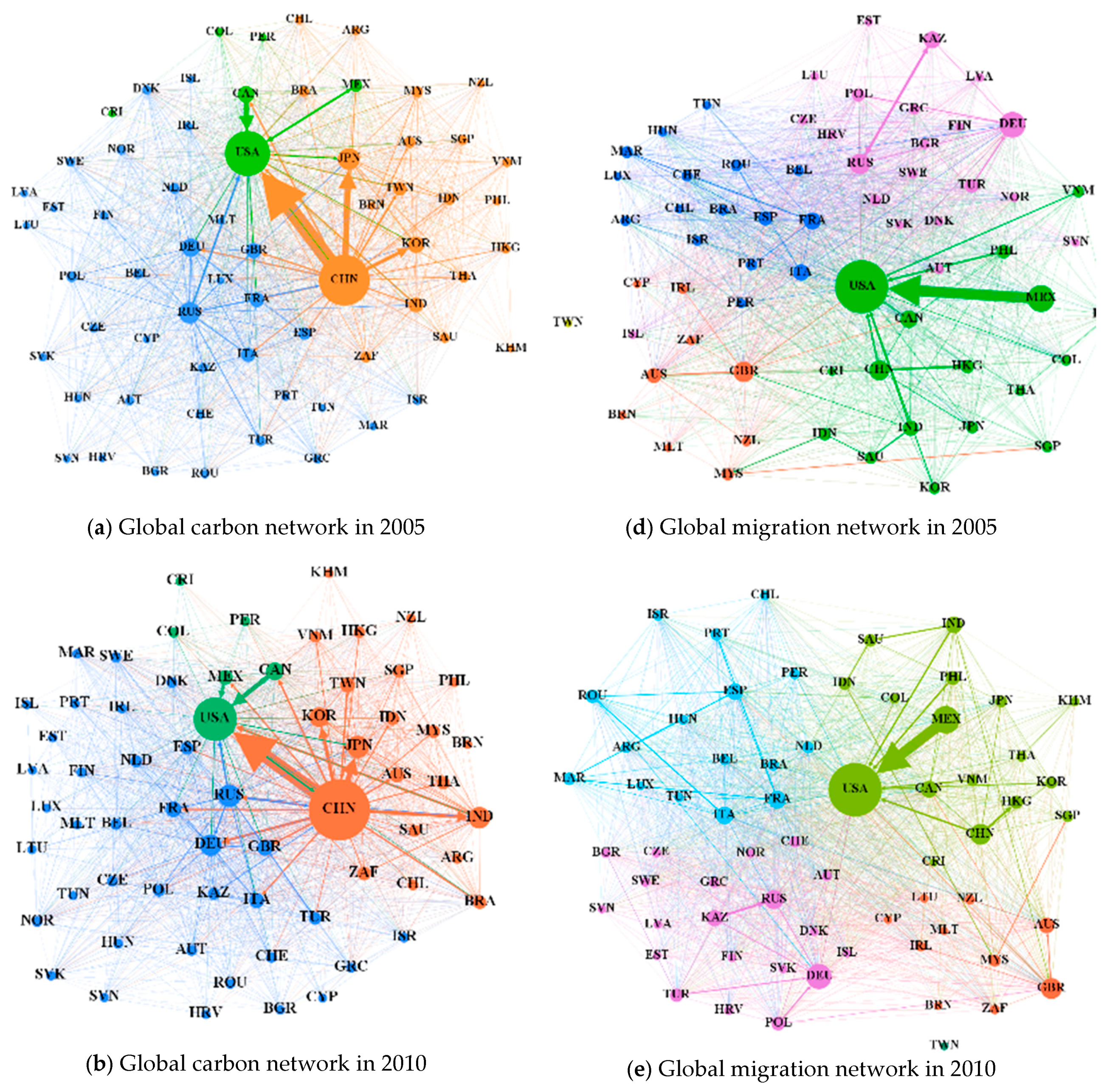
  • First, based on gravity concept and two-layer network method, we investigate the structural similarity between the global migration network and the carbon transfer network.
  • Second, we use the STIRPAT framework to analyze the impact of migration on embodied carbon transfers.
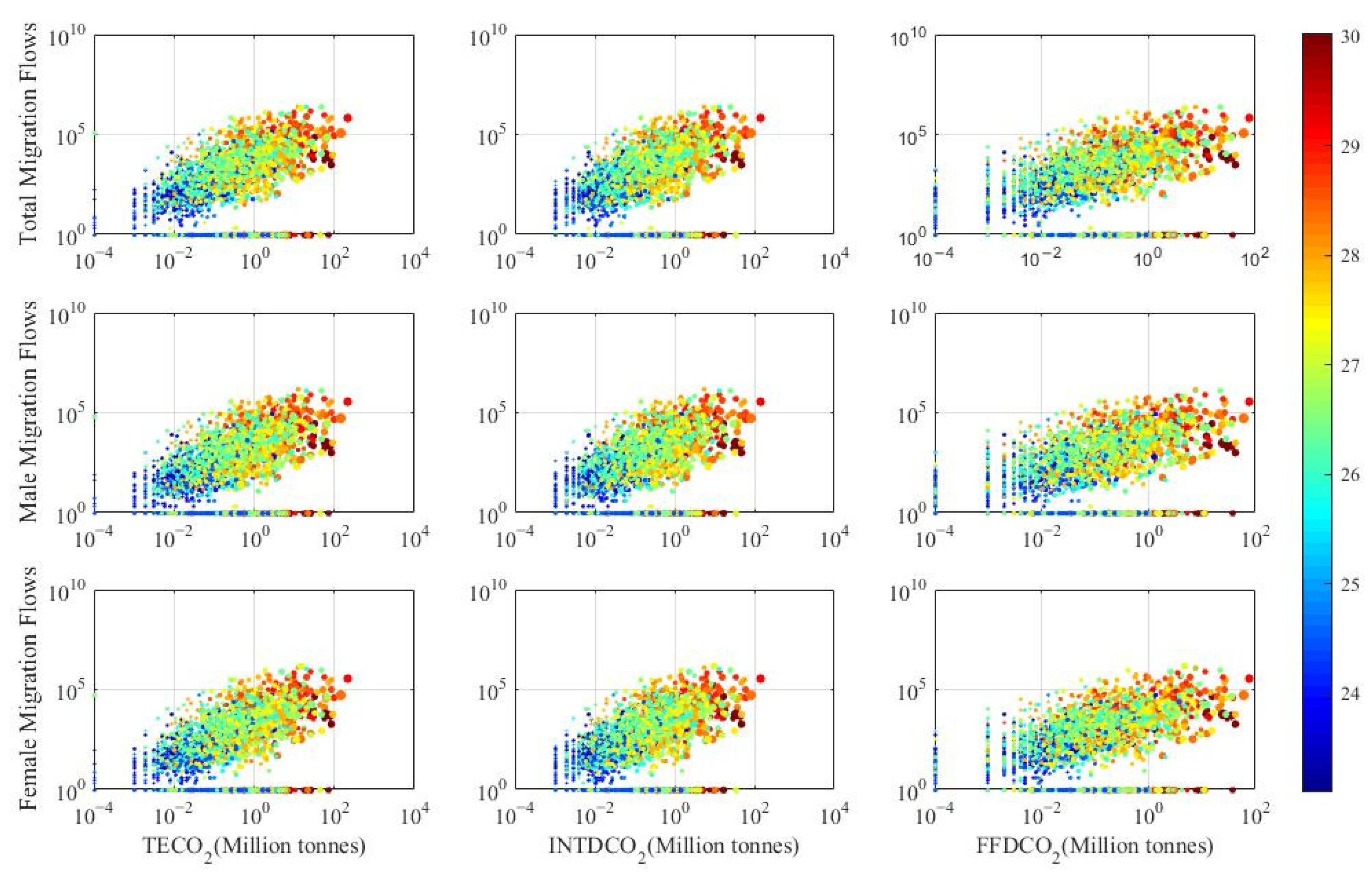
  • Third, we discuss the implications of heteroscedastic impacts induced by gender, income levels, and product composition.
The remaining sections of the study are structured as follows; Section 2 presents our methodology and data sources. Section 3 further elaborated the main empirical results whereas the Section 4 centers on the results discussion. The last section concludes this research.

2. Methodology and Data

2.1. Two-Layer Network and Dissimilarity Metric

Specifically, the study models migration and carbon transfer systems by a network of G = (V,E), where V and E represent the set of nodes and edges, respectively. W (with element of w ij ) is thus denoted as the adjacency matrix of G. Furthermore, w ij represents the migrants and carbon transfers, which aids in obtaining a weighted and directed two-layer network. To display similar or different characteristics between two network layers, the structural dissimilarity is calculated. Notably, dissimilarity metric (D-measure) is a quantitative and effective measure for multiplex network comparison [27,28]. The structural dissimilarity can be measured based on the link weighted-based difference and the connection-based difference. According to Ref. [29], the node dissimilarity can firstly be computed using the node’s probability distribution vector. The whole network difference between two different networks is then obtained based on all nodes’ dissimilarities.
Specifically, the weighted-based vector ( Pw i k ) is transformed in the k -layer network to a probability distribution as follows:
Pw i k = ( w i 1 k / S i k , w i 2 k / S i k , , w iN k / S i k ) ,   and   S i k = j = 1 N w ij k  
where N represents the total number of nodes; w ij k is the edge weight between node   i   and   j , j = 1 , , N ; and S i k is the strength of node i .
Similarly, the connection-based probability distribution vector ( Pc i k ) of node i in the k -layer network can be calculated as:
Pc i k = ( d i 1 k / D i k , d i 2 k / D i k , , d iN k / D i k ) ,   and   D i k = j = 1 N d ij k
where D i L represents the node degree (the number of links incident on node i , in the L -layer network). Notably, d ij k = 1 if node i and j are connected, and d ij k = 0 , if otherwise.
The two metrics of weighted-based dissimilarity ( WND i L   L ) and connection-based dissimilarity ( CND i L   L ) for node i between the two-layer networks of L   and   L are thus calculated correspondingly as:
WND i L   L = 1 2 j = 1 N ( Pw ij L Pw ij   L ) 2
CND i L   L = 1 2 j = 1 N ( Pc ij L Pc ij   L ) 2
where for k =   L and   L , Pw ij k and Pc ij k are components of vectors   Pw i k   and   Pc i k   respectively .
Finally, the whole network metrics of the weighted-based dissimilarity ( WD LL ) and connection-based dissimilarity ( CD L L ) between L -layer and L -layer networks are calculated respectively as;
WD LL = i = 1 N α i LL WND i LL ,   and   α i LL = W i L L j = 1 n W j L L
CD L L = i = 1 N β i L L CND i L L ,   and   β i L L = D i L L j = 1 n D j L L
where WD LL [ 0 , 1 ] , CD LL [ 0 , 1 ] ; W i L L = W i L · W i   L   and D i L L = D i L · D i L represent the geometric mean between the corresponding metrics in two different layers.
Hence, the larger the values of   WD LL and CD L L , the greater the dissimilarity between the two-layer networks. Similarly, the connection-based out- and in-dissimilarity together with the weighted-based out- and in-dissimilarity can be defined.

2.2. Environmental Impact of Migration: A STIRPAT Model

IPAT model is a typical quantitative model proposed by Ehrlich and Holdren in the 1970s to measure the impact of population, affluence, and technology factors on the environment. Specifically, the IPAT model overcame the shortcoming of Laspeyres index decomposition method, which can only reflect the changes of one factor. Nevertheless, the IPAT model brought new challenges since it just reflects the proportional influence among variables. In order to overcome the limitations of the IPAT model, Dietz and Rosa constructed the Stochastic Impacts by Regression on Population, Affluence, and Technology (STIRPAT) model by introducing a nonlinear index to portray the non-proportional influences [30].
In a panel data framework, logarithmic transformation can linearize the trend of data without changing the data characteristics. The log-transformed panel data can also help to directly obtain the elasticity of dependent variable in relation to the independent variable(s) directly. Hence, the Log-linearized STIRPAT model can be written as Equation (7).
  lnI = ε + α lnP + β lnA + γ lnT
where I , P ,   A , and T represent environmental impacts, population, affluence, and technology, respectively. From this point of view, various indicators are used to represent each component of STIRPAT (e.g., Lin et al., (2009) [31]; Li et al., (2011) [32]; Shabaz et al., (2016) [33]; and Ulucak et al., (2021) [34]).
In this paper, the STIRPAT model is regarded as the theoretical analysis framework. The population ( P ) factor is therefore further divided into two aspects: population scale (POP) and population migration (PM). A from the STIRPAT model is depicted by per capita gross domestic product (rGDP), T is technology represented by foreign direct investment (FDI) while I represents embodied carbon emission transfers (CT). Different scholars define technology factors with different methods. In this paper, the FDI is used to assess technology level because it brings in more advanced production technology.
Equation (7) can therefore be extended to form Equation (8a) as;
Model 3:
ln ( C T i j ) = ε + α 1 ln ( PM i j ) + α 2 ln ( POP i ) + α 3 ln ( POP j ) + β 1 ln ( rGDP i ) + β 2 ln ( rGDP j ) + γ 1 ln ( FDI i ) + γ 2 ln ( FDI j )
where CT i j and PM i j represent carbon emission transfers and population mobility between country i and j , respectively. POP i ,   rGDP i , and FDI i represent total population scale, per capita GDP and FDI for country i . α 1 ,   α 2 ,   α 3 ,   β 1 , . β 2 ,   γ 1 and γ 2 represent elasticity coefficients pertaining to the corresponding explanatory variables as specified in Equation (8a).
Prior to estimating the study’s full model as specified in Equation (8a), two additional models are developed from the full model in a hierarchy or stepwise manner as follows;
Model 1:
ln ( CT i j ) = ε 1 + α 1 ln ( PM i j ) + α 2 ln ( POP i ) + α 3 ln ( POP j ) +   β 1 ln ( rGDP i ) + β 2 ln ( rGDP j )
Model 2:
ln ( CT i j ) = ε 3 + α 1 ln ( PM i j ) + α 2 ln ( POP i ) + α 3 ln ( POP j ) +   β 1 ln ( rGDP i ) + β 2 ln ( rGDP j ) + γ 1 ln ( FDI i )
Since different models in stepwise manner have been formulated, there is a need to select the best one or the model which performs more efficiently [35,36]. Results pertaining to Equation (8a) are outlined in Table 1, Table 2 and Table 3 as Model 1, Model 2, and Model 3 correspondingly. Based on this assertion, the Akaike information criterion (AIC) approach is employed. Specifically, the AIC approach is an estimator of prediction error and thereby relative quality of statistical models for a given data set [37,38]. Given a collection of models for a specific data, AIC estimates the quality of each model relative to each of the other models. Thus, AIC provides a means for model selection. Theoretically, suppose that we have a statistical model of some data, let k be the number of parameters in the model. Also let L ^ be the maximum value of the likelihood function for the model. Then the AIC value of the model can be computed using the following relation;
AIC = 2 k 2 ln ( L ^ )
Thus, given a set of candidate models for the data, the preferred model is the one with minimum AIC value.

2.3. Data Source

The data for 2005, 2010, and 2015 used in this paper involves carbon flows embodied in trade and population migration between countries, together with national population scale, GDP and FDI. Carbon dioxide emissions embodied in international trade (TECO2) is divided into two different types: (i) domestic emissions embodied in exports of intermediate products (INTDCO2) and (ii) domestic emissions embodied in foreign final demand (FFDCO2). Data pertaining to the embodied carbon flows was downloaded from the Organization for Economic Cooperation and Development (OECD), which involves 64 countries (unit in million tons) [39]. The OECD database is a consistent global database that contains input-output tables, bilateral carbon dioxide trade data, and other national accounts data. Due to the complexity of inter-sector and inter-country carbon flows, the latest main data sources (2019 edition of the OECD) in the period from 2005 to 2015 is used. The list countries, country codes, and sub-regions can be found in Appendix A (see Table A1).
Further, migration data was derived from the United Nations [40]. The United Nations Global migration database comprises of a comprehensive empirical data of international migration for more than 200 countries by birth and citizenship, sex, and age, during the period of 1990–2019.
Additionally, the data for national population scale, per capital real GDP (with constant 2015 USD), and FDI is as well be obtained from the World Development Indicators (World Bank, 2021) [41]. In the progressive regression of Equation (9), the data and corresponding variables description are presented in Appendix A Table A2.

3. Empirical Results

3.1. Center-of-Gravity Movement and Comparison

In this section, the distribution characteristics and dynamic evolution of carbon transfers induced by trade among 64 countries based on the “center-of-gravity” theory are examined. A comparative analysis concerning the trajectory of carbon transfer centers and population migration centers is further conducted. The concept of “center-of-gravity” is an important tool for analyzing the spatial distribution. The centers with respect the “center-of-gravity” move around of regional pattern, which is a geometric property and originated from physics [42,43]. According to the changes in the gravity centers, the space-time similarity or inconsistency between embodied carbon flows and migration flows can be depicted. The center-of-gravity can therefore be computed using the following relations:
X T =   X i W i T   W i T ,       Y T =   Y i W i T   W i T
where X T and Y T represent the latitude and longitude of the center-of-gravity in year T. W i T represents the property for country i. X i and Y i represent the geographical locations of country i and country j, which are expressed by the geometric center of the countries. Here, the geometric center is defined by administrative boundaries. In this paper therefore, the Arcgis, a geometric computation method, is used to protract the center-of-gravity as well as their moving trajectories, as shown in Figure 1.
As evidenced in Figure 1, the centers of import- and export-induced carbon transfers are close—with the same latitude and about 30 degrees difference in longitude. The centers of import-induced carbon transfers are closer to western developed countries (this is indicated using red circles). This thus may suggest that, developed economies transfer carbon emissions by importing a large number of intermediate products. The centers of export-induced carbon transfers are located in Central Asia (indicated using yellow circles), which is mainly affected by the product export characteristics of developing countries, especially China.
Moreover, both import- and export-induced carbon transfers depicted similar evolution trend in gravity centers, which moved towards the southeast with a “fast-first, slow-later” pattern. This as a result confirms the role of China as larger importer and exporter of carbon sequestration among developing countries. However, the movement rate of the center-of-gravity of import-induced carbon transfer slowed significantly from 2010 to 2015. In 2015, the global economy was sluggish with the surge in primary energy consumption well below the 10-year average. Other energy sources such as nuclear power, hydroelectric power, wind power, solar power, and biofuel are evidenced to be developing steadily. As a result, global carbon transfers are growing at the slowest rate.
Similar to carbon transfers, the center-of-gravity of global population migration has the same characteristics (these are illustrated in Figure 1 using green and purple circles). The centers of immigration located in the west of emigration, indicates that the main destinations of international migration are western developed countries. Besides, the evolutionary path of migration center is consistent with the distribution of major oil producing countries who attract a large number of foreign labor force. More importantly, the velocity of the centers speeds up with respect to the development of Asian countries, which attract foreign investment and immigration. However, the center of emigration moving faster, implies that high foreign investment and a large amount population moved out in developing countries, most notably China. Generally, the gravity centers of carbon transfers and migration tend to move in the same direction.

3.2. Inter-Layer Network Dissimilarity Analysis Based Nodes

To verify the relationship between global migration network (GMN) and global carbon network (GCN), we analyze their structural difference with the help of network dissimilarity measurements. Figure 2 therefore shows that, compared with GCN, the GMN exhibit multi-centralization characteristics. In addition, the two kinds of networks show globalization in terms of the connectivity of inbound and outbound links. That is, the vast majority of the country pairs are accompanied by inflows or outflows, but with link weights heterogeneity. This result is consistent with the power-law conclusions from the vast majority of research in energy trade and migration networks (see for example references [19,44,45]). There is, therefore, no need repeat the topology of single-layer network, but rather focus on comparing different networks.
In order to make the cross-county comparison easy, the structural in- and out-dissimilarity across countries are further measured. Based on the definition of structural difference between the same nodes in different networks, the overall network dissimilarity, as well as the data of population migration and carbon emission transfer between 64 countries in three different years, we calculated the structural difference for each country from the perspective of export and import, as shown in Figure 3. The overall network structural difference between the two-layer networks is further measured, as shown by the radar maps (see Figure 3).
From Figure 3, the structural in- and out-differences for countries between the two layers range from 0.2 to 0.8, with an average value of 0.5. Figure 3 further depicts that the distribution of weighted links pertaining to the countries such as, BRN, SAU, TWN, RUS, MYS, etc., differ greatly between the two layers of GCN and GMN. On the contrary, countries including LTU, CAN, SWE, BGR, AUT, etc., have the same or less differentiated weighted links distribution. Generally, the values concerning the structural out-dissimilarity are similar to that of in-dissimilarity. However, there are still some obvious distinctions between structural in-dissimilarity and out-dissimilarity in the case of KAZ, THA, TUN, IDN, CHN, LUX, FRA, and CAN. This distinction is caused by the resources and economic characteristics pertaining the specific country. With respect to the network’s total structural dissimilarity, the values marginally vary over time from 0.2–0.4, except for the export structure in 2005.

3.3. Inter-Layer Network Similarity Analysis Based Links

Figure 4 moreover shows the scatter diagram of connected links concerning the two kinds of networks. Besides, carbon emissions embodied in international trade is sub-divided into two types, namely INTDCO2 and FFDCO2. The total population migration is also divided into male and female in order to investigate gender’s influences.
The nine subgraphs in Figure 4 show that there is a positive correlation between migration and trade-induced carbon transfers. In other words, the connection between two countries with larger carbon flows is usually accompanied by larger numbers of migrants. Moreover, Figure 4 shows that links with similar GDP for destinations (the same color) are adjacent and increasing along the diagonal from the lower left to the upper right corner. Simultaneously, the marker size increases with the color turning from blue to red. This insinuates that trade-induced carbon transfers are affected by economic and population factors. Certainly, many scholars have verified this conclusion (see for example references [12,13,48]).
Therefore, it is necessary to evaluate the impact of population migration on carbon emission transfer comprehensively by means of econometric model. Specifically, the effects of gender and income level on the carbon emissions embodied in international trade are also discussed in detail (see Section 4).

3.4. Regression Results of Migration’s Effect on Carbon Transfers

Based on the model specified in Equation (8a), total population scale, per capita GDP, and population migration are taken as the independent variables, whereas technical level is taken as control variable. The Eviews software is used for the stepwise regression analysis. During the regression process, all variables are transformed to natural logarithm to eliminate heteroscedasticity issues. If the positive and negative coefficients of the original variables do not change after adding variables one by one, then there is an indication that the full model is robust. Since the series of regression models in a stepwise manner are estimated prior to the full model, the AIC approach is as well employed to detect which of the models specified is most efficient and robust enough.
Like existing studies, results with respect to the traditional factors including population scale and per capita GDP driving the transfer of carbon, are shown in Table 1, Table 2 and Table 3. The impact of population scale in origins is slightly lower than that concerning destinations with elasticities within the ranges 0.741–0.845 and 0.789–0.865, respectively. Moreover, the driving force of origins shows “decrease-first, increase-later” pattern while that of destinations is increasing. The elasticity coefficients of per capita income for origins and destinations are more different, ranging from 0.567–0.692 and 0.737–0.779, correspondingly. This indicates that the economic development level of carbon emission importing countries is the main driving force of carbon emission transfer. Under the global division of labor, developing countries are victims of “high pollution, high consumption, and high emissions” in the global low-end manufacturing sector. The shift of high-emission industries or low-end manufacturing makes developing countries a front for carbon transfer. Therefore, in order to change the existing pattern, developing countries must take various measures, such as technological research and development, industrial upgrading of export-oriented economy, vigorously developing low-carbon export economy, and green export economy, as well seize the commanding heights of the value chain.
In addition, Models 2 and 3 show that FDI i has a significant positive impact on carbon transfers, although its impact was much smaller than the above two factors. In other words, the upsurge in FDI concerning the origins promotes the transfer of carbon from origins to destinations. Specifically, the estimates with respect to FDI i decreases. The results show that for every 1% increase in FDI i , the carbon outflow will increase by approximately 0.254%, 0.232%, and 0.073%, respectively. This can be interpreted as in the process of economic globalization, the destinations (mainly developed countries) use the cheap labor force of the origins (mainly developing countries) for capital input. Developing countries thus produce products, while developed countries transfer carbon through imports. This therefore suggests that the influence of FDI on carbon transfers is greater in the origins. Generally, the total population scale for origins and destinations have a comparative positive effect on carbon transfers. Nonetheless, there are significant differences for per capita income and FDI.
In the case of migration, results from Model 1 to Model 3 depicts that worldwide population migration has a positive effect on the flow of embodied carbon emissions. This positive promoting effect becomes stronger as total migration scale increases. The regression results with respect to each of the three years show that1% increase in population migration increases carbon emission transfer by 0.118%, 0.118%, and 0.124%, respectively. The effects of migration are gradually increasing and becoming extremely obvious. As people move in, the demand for life-form energy increases, along with the increasing consumption of traded products, thus contributing to the inflow of more carbon emissions. On the other hand, the influx of a large number of immigrants may cause a shortage of housing in the host country, and to a certain extent, increase the construction of residential and urban infrastructure, thus requiring a large number of building materials with higher energy consumption and emissions, such as the cement industry. In 2010 for instance, the elasticity coefficient concerning the impact of migration on carbon transfers showing no apparent increase. The main reason is that the global financial markets affect human migration, through the labor force market for instance [49].
Finally, post estimation checks based on the F-test together with the R2-adjusted indicates that all the estimated models for the respective years are correspondingly good fit compared to an empty model. Considering the multiple models estimated, there is a need to select the best. Thus, as already mentioned the AIC approach was adopted. Evidently, results from Table 1, Table 2 and Table 3 unveils that among the series of model estimated in a stepwise manner, the full model (Model 3) recorded the least AIC value for all the respective years. It is therefore possible to infer that the study’s full model is most efficient and as well robust to rely on in terms of estimating the determinants of carbon dioxide emission transfer.

4. Discussions

This section discusses our findings in two steps. The previous analysis showed that population migration has a positive effect on bilateral carbon flows. This may suggest that the international population migration is generally manifested from countries of lower income to developed countries. Migrants from countries with lower development level often choose to emigrate for the purpose of raising income level and improving living conditions, while migrants from developed countries choose to emigrate mostly for their own personal needs and preferences. The motivations between different countries with varying development levels may also have different impacts on carbon flows. Based on these outcomes we endeavor to answer the following questions: (i) What is the impact of internal migration on carbon flows among the same income economies? (ii) What is the impact of migration among different income economies on their carbon flows? (iii) Does gender migration also have a different impact on the carbon emissions embodied in intermediate and final products trade? These outlined questions will be discussed in the subsequent sections in detail.

4.1. Impact of Sex-Specific Migration

To determine if the sex-specific migration influence carbon flows embodied in intermediate and final products, we employed INDCO2 and FFDCO2 as independent variables respectively. Precisely, the total migration is replaced with male migration or female migration. The afore-mentioned regression method is again employed in this scenario to obtain models for different years. Figure 5 thus shows the elastic coefficient concerning the impact of gender migration on carbon transfers from 2005 to 2015. In general, the two types of carbon flows are positively promoted by migration, but the carbon embodied in intermediate products is more affected.
The results indicate:
First, the driving force of migration on carbon transfers gradually shows significant gender differences. Furthermore, the driving effect of male migration on carbon transfer is slightly greater than that of female migration. The difference is thus evidence to be an increasing trend (see Figure 5a,b). This outcome may imply that, many international migrants are motivated by raising income and improving living conditions. Men and women are mainly engaged in different jobs, hence their impact on carbon transfers will also be different.
Second, the pattern with regards to the impact of migration on the two types of carbon transfer remains unchanged. That is, the impact of migration on the carbon emissions induced by exporting intermediate products is greater than that of final products, and the difference between them is gradually witnessed to be increasing, as shown in Figure 5c and Figure 5d correspondingly. This therefore means that, with the mobility of population, the demand for intermediate products in the host country becomes greater. This can also be interpreted as international immigrants who provide labor force for the host country, are mainly engaged in the production and processing of products. Similarly, developing countries lag behind in economy, science, and technology, together with the export of more intermediate products. With the improvement of people’s consumption level, their demand for various products increases. More and more immigrants are engaged in tertiary industries such as service industry, but in comparison, intermediate products are in greater demand.
Third, according to the four graphs in Figure 5, the impact of migration on carbon transfers induced by both intermediate and final products decreased significantly in 2010. This may be due to the impact of the global economic crisis in 2008. The trade of products during the mentioned year was affected and has not recovered to the original level in a short time.

4.2. The Heteroscedasticity of Migration’s Affect across Income Levels

In order to analyze the heteroscedasticity of migration’s influences across income levels, this section classifies 64 countries into three groups (denoted by group I-III) based on income levels as: High income economics (HIEs), Upper middle-income economies (UMEs), together with Low and lower middle income economies (LMEs), with 42, 15, and 7 countries in each group, respectively. Details concerning the income level divisions for the listed 64 countries are provided in Table A1. We therefore discuss three intragroup cases: Case I (Figure 6a), Case II (Figure 6e), and Case III (Figure 6i); and six intergroup cases: Case I-II, Case I-III, Case II-I, Case II-III, Case III-I, and Case III-II. Regression analysis was conducted for each situation according to the already mentioned technique.
Evidence from Figure 6 indicates that, the impact of migration in Case III fluctuates greatly compared with Case I and Case II. At the same time, the more developed the economy, the lower the elasticity. This may be due to the fact that HIEs have more advanced technology and complete infrastructure. Hence, the influx of migrants will not cause problems such as housing shortages, thus holding energy use compared with UMEs and LMEs. Meanwhile, advanced technology has reduced carbon emissions by increasing resource utilization. This therefore will not cause a large increase, although the inflow of immigrants may lead to an increase in daily necessities and carbon transfers. As a result, the elastic coefficient in Figure 6a is less than 0.2.
Considering the results among different groups, we deduce that:
Firstly, the elasticity of Case I-II was significantly lower than that of Case II-I. This may imply that globalization has facilitated the relocations of factories from high income nations to upper middle income nations by multinational corporations. Nonetheless, the elasticity of Case I-II increased slightly while that of Case II-I decreased (see Figure 6b,d. This shows that the migration of population from upper middle-income countries to high income countries has a greater impact on carbon transfers, but this impact decreased.
Secondly, the regression coefficients in Figure 4d,h continue to decline. To some extent, this indicates that populations moving from less developed countries to more developed countries have a decreasing impact on carbon flows. Although in the early stages of migration, population mobility may cause problems such as housing shortage in less developed countries; nonetheless, this effect is small and will diminish. From the perspective of motivation, in addition to individual needs, it is largely recommended to make some investment to take advantage of cheap labor. This would slow the spread of climate-change technologies.
Thirdly, the elasticity of Case I-III and Case III-I have a same tendency. Nonetheless, the elasticity of Case I-III was significantly higher than that of Case III-I. The largest positive impact occurs between UMEs and LMEs.
In conclusion, the impact of population migration varies greatly among groups with different income levels. Therefore, economic development as well as gender need to be considered in the study of population migration and spatial carbon emission transfers.

5. Conclusions and Implications

This paper provides a quantitative assessment pertaining to the effect of international migration on embodied carbon emission transfers, using the STIRPAT framework, combined with complex network theory. The results of this study provide a new view for further carbon emission analysis from the perspective of demographic factor.
Through the analysis of stepwise regression model, it is evidenced that the traditional factors, such as population scale and GDP, are the leading factors of embodied carbon flows between countries, with positive effects on carbon transfers correspondingly.
Importantly, population migration and trade-induced carbon flows were positively relevant. Namely, every 1% increase in population flow will increase carbon transfers by about 0.12%. This outcome indicates that population mobility between countries will aggravate the codirectional flow of carbon transfers. This is especially true between high-income and low-income countries. Therefore, compared with developing countries, developed countries should take migration factor into account when formulating population policies. However, from the perspective of climate change, the outflow of population makes the carbon emissions caused by exporting products in the host country, which should be re-measured by joint responsibility. The responsibility accounting system of carbon emissions should be improved according to the characteristics of each country’s development stage and the principle of “common but different”.
Moreover, the impact of population migration on carbon emission transfer among countries at the same income level will be different with the level of income. In other words, the higher the income level, the smaller the impact. Specifically, the global financial crisis has affected this relationship. In other words, the financial crisis is harmful to migration’s positive effect from UMEs to HIEs (see Figure 6d) and LMEs (see Figure 6f), while benefit to migration’s positive effect between HIEs and LMEs (see Figure 6c,g). This led to a slight change in the worldwide impact of migration on carbon transfers in 2010.
In all, we believe that population migration increases the transfer of trade-induced carbon emissions, especially for intermediate carbon transfers. Thus, the resulting potential environmental problems deserve to be considered by governments in their policy formulation. If migration factor is excluded, carbon transfers embodied in trade will be underestimated. Based on this research, we deem that countries should adopt differentiated measures (based on income level) to reduce the growth of carbon emissions from migration according to their respective stages of development. In the face of global climate change, developed countries should take the lead in emission reduction and export emission reduction technologies and as well as provide assistance to countries with lower development levels and emerging economies, so as to shoulder more international responsibilities in addressing global climate change. At the same time, the study of the population–economy–environment analytical structure should be strengthened.

Author Contributions

Conceptualization and methodology, C.G. and Y.Z.; software, S.T. and Y.H.; validation, I.A.M.; writing, Y.Z.; supervision, C.G. All authors have read and agreed to the published version of the manuscript.

Funding

This research was funded by the National Natural Science Foundation of China, grant number 71804060.

Institutional Review Board Statement

Not applicable.

Informed Consent Statement

Not applicable.

Data Availability Statement

Acknowledgments

The authors gratefully acknowledge the financial support from the National Natural Science Foundation of China (Grant no. 71804060) and a project funded by the Priority Academic Program Development of Jiangsu Higher Education Institutions (No. PAPD-2018-87).

Conflicts of Interest

The authors declare no conflict of interest. The funders had no role in the design of the study; in the collection, analyses, or interpretation of data; in the writing of the manuscript, or in the decision to publish the results.

Appendix A

Table A1. List of 64 countries involved in this paper.
CountryAbbreviationRegionCountryAbbreviationRegion
42 High income economics (HIEs)
AustraliaAUSEast Asia and
the Pacific
AustriaAUTEurope and Central Asia
Brunei DarussalamBRNBelgiumBEL
Hong Kong, ChinaHKGCroatiaHRV
JapanJPNCyprusCYP
New ZealandNZLDenmarkDNK
SingaporeSGPEstoniaEST
CanadaCANNorth AmericaFinlandFIN
IsraelISRMiddle East and
North Africa
FranceFRA
United StatesUSASlovakiaSVK
Republic of KoreaKORTaiPei, ChinaTWN
MaltaMLTGermanyDEU
Saudi ArabiaSAUGreeceGRC
NorwayNOREurope and Central AsiaHungaryHUN
PolandPOLIcelandISL
PortugalPRTIrelandIRL
SloveniaSVNItalyITA
SpainESPLatviaLVA
SwedenSWELithuaniaLTU
SwitzerlandCHELuxembourgLUX
United KingdomGBRNetherlandsNLD
CzechiaCZE
ChileCHLLatin America and the Caribbean
15 Upper middle income economies (UMEs)
ArgentinaARGLatin America and the CaribbeanChinaCHNEast Asia and
the Pacific
BrazilBRAMalaysiaMYS
ColombiaCOLThailandTHA
Costa RicaCRIBulgariaBGREurope and Central Asia
MexicoMEXKazakhstanKAZ
PeruPERRomaniaROU
South AfricaZAFSub-saharan AfricaTurkeyTUR
RussiaRUSEurope and Central Asia
7 Low and lower middle income economies (LMEs)
IndonesiaIDNEast Asia and
the Pacific
IndiaINDSouth Asia
CambodiaKHMMoroccoMARMiddle East and North Africa
PhilippinesPHLTunisiaTUN
Viet NamVNM
Table A2. Definition of the variables.
Types of VariablesVariablesDefinitions
Explained variableCarbon emission transfers (CT)Embodied carbon emissions flows
Explanatory variablesPopulation scale (POP)Total population size
Economic development level (rGDP)GDP/total population
Population migration (PM)Migration flows
Control variableTechnical progress (FDI)Foreign direct investment

References

  1. Gazzotti, P.; Emmerling, J.; Marangoni, G.; Castelletti, A.; Wijst, K.V.D.; Hof, A.; Tavoni, M. Persistent inequality in economically optimal climate policies. Nat. Commun. 2021, 12, 3421. [Google Scholar] [CrossRef] [PubMed]
  2. United Nations Climate Change. Available online: https://unfccc.int/ (accessed on 20 March 2020).
  3. Zhang, C.; Zhou, X. Does foreign direct investment lead to lower CO2 emissions? Evidence from a regional analysis in China. Renew. Sustain. Energy Rev. 2016, 58, 943–951. [Google Scholar] [CrossRef]
  4. Wang, M.; Feng, C. Decomposition of energy-related CO2 emissions in China: An empirical analysis based on provincial panel data of three sectors. Appl. Energy 2017, 190, 772–787. [Google Scholar] [CrossRef]
  5. Lv, Y.; Chen, W.; Cheng, J. Modelling dynamic impacts of urbanization on disaggregated energy consumption in China: A spatial Durbin modelling and decomposition approach. Energy Policy 2019, 133, 110841. [Google Scholar] [CrossRef]
  6. Abeydeera, L.H.U.W.; Mesthrige, J.W.; Samarasinghalage, T.I. Global Research on Carbon Emissions: A Scientometric Review. Sustainability 2019, 11, 3972. [Google Scholar] [CrossRef] [Green Version]
  7. Ehrlich, P.R.; Holdren, J.P. Impact of population growth. Science 1971, 171, 1212–1217. [Google Scholar] [CrossRef]
  8. Kaya, Y. Impact of Carbon Dioxide Emission Control on GNP Growth: Interpretation of Proposed Scenarios [R]. Presented at the Energy and Industry Subgroup, Response Strategies Working Group, International Panel on Climate Change, Paris, France; 1990. Available online: https://archive.ipcc.ch/publications_and_data/publications_ipcc_first_assessment_1990_wg3.shtml (accessed on 20 March 2020).
  9. Wang, Y.; Zhao, H.; Li, L.; Liu, Z.; Liang, S. Carbon dioxide emission drivers for a typical metropolis using input–output structural decomposition analysis. Energy Policy 2013, 58, 312–318. [Google Scholar] [CrossRef]
  10. Fang, D.; Yang, J. Drivers and critical supply chain paths of black carbon emission: A structural path decomposition. J. Environ. Manag. 2021, 278, 111514. [Google Scholar] [CrossRef] [PubMed]
  11. Zhang, X.; Li, Z.; Ma, L.; Chong, C.; Ni, W. Analyzing Carbon Emissions Embodied in Construction Services: A Dynamic Hybrid Input–Output Model with Structural Decomposition Analysis. Energies 2019, 12, 1456. [Google Scholar] [CrossRef] [Green Version]
  12. Dong, F.; Yu, B.; Hadachin, T.; Dai, Y.; Wang, Y.; Zhang, S.; Long, R. Drivers of carbon emission intensity change in China. Resour. Conserv. Recycl. 2018, 129, 187–201. [Google Scholar] [CrossRef]
  13. Yu, B.; Wei, Y.M.; Kei, G.; Matsuoka, Y. Future scenarios for energy consumption and carbon emissions due to demographic transitions in Chinese households. Nat. Energy 2018, 3, 109–118. [Google Scholar] [CrossRef]
  14. Hauer, M.E. Migration induced by sea-level rise could reshape the US population landscape. Nat. Clim. Chang. 2017, 7, 321–325. [Google Scholar] [CrossRef] [Green Version]
  15. Black, R.; Adger, W.N.; Arnell, N.W.; Dercon, S.; Geddes, A.; Thomas, D. The effect of environmental change on human migration. Glob. Environ. Chang. 2011, 21, S3–S11. [Google Scholar] [CrossRef]
  16. Stephenson, J.; Newman, K.; Mayhew, S. Population dynamics and climate change: What are the links? J. Public Health 2010, 32, 150–156. [Google Scholar] [CrossRef] [PubMed]
  17. Sun, Y.; Zhang, X.; Ding, Y.; Chen, D.; Qin, D.; Zhai, P. Understanding human influence on climate change in China. Natl. Sci. Rev. 2021, nwab113. [Google Scholar] [CrossRef]
  18. Huwart, J.Y.; Verdier, L. Economic Globalisation: Origins and Consequences [D]; OECD Insights; OECD Publishing: Paris, France, 2013; ISBN 9789264111899. [Google Scholar]
  19. Sgrignoli, P.; Metulini, R.; Schiavo, S.; Riccaboni, M. The relation between global migration and trade networks. Phys. A Stat. Mech. Appl. 2015, 417, 245–260. [Google Scholar] [CrossRef] [Green Version]
  20. Li, Q.; Chen, H. The Relationship between Human Well-Being and Carbon Emissions. Sustainability 2021, 13, 547. [Google Scholar] [CrossRef]
  21. Lebel, L.; Garden, P.; Banaticla, M.R.N.; Lasco, R.D.; Contreras, A.; Mitra, A.P.; Sharma, C.; Nguyen, H.T.; Ooi, G.L.; Sari, A. Integrating carbon mangement into thedevelopment strategies of urbanizing regions in Asia. J. Ind. Ecol. 2007, 11, 61–81. [Google Scholar] [CrossRef] [Green Version]
  22. Noja, G.G.; Cristea, S.M.; Yüksel, A.; Pânzaru, C.; Drăcea, R.M. Migrants’ Role in Enhancing the Economic Development of Host Countries: Empirical Evidence from Europe. Sustainability 2018, 10, 894. [Google Scholar] [CrossRef] [Green Version]
  23. Gao, C.; Tao, S.; He, Y.; Su, B.; Sun, M.; Mensah, I.A. Effect of population migration on spatial carbon emission transfers in China. Energy Policy 2021, 156, 112450. [Google Scholar] [CrossRef]
  24. Shi, G.; Lu, X.; Deng, Y.; Urpelainen, J.; Liu, L.C.; Zhang, Z.; Wei, W.; Wang, H. Air Pollutant Emissions Induced by Population Migration in China. Environ. Sci. Technol. 2020, 54, 6308–6318. [Google Scholar] [CrossRef]
  25. Benveniste, H.; Oppenheimer, M.; Fleurbaey, M. Effect of border policy on exposure and vulnerability to climate change. Proc. Natl. Acad. Sci. USA 2020, 117, 26692–26702. [Google Scholar] [CrossRef] [PubMed]
  26. Liu, B.; Zhao, Q.; Jin, Y.; Shen, J.; Li, C. Application of combined model of stepwise regression analysis and artificial neural network in data calibration of miniature air quality detector. Sci. Rep. 2021, 11, 3247. [Google Scholar] [CrossRef]
  27. Schieber, T.A.; Carpi, L.; Díaz-Guilera, A.; Pardalos, P.M.; Masoller, C.; Ravetti, M.G. Quantifcation of network structural dissimilarities. Nat. Commun. 2017, 8, 13928. [Google Scholar] [CrossRef] [Green Version]
  28. Jiang, Y.; Li, M.; Fan, Y.; Di, Z. Characterizing dissimilarity of weighted networks. Sci. Rep. 2021, 11, 5768. [Google Scholar] [CrossRef]
  29. Zhang, X.; Cui, H.; Zhu, J.; Du, Y.; Wang, Q.; Shi, W. Measuring the dissimilarity of multiplex networks: An empirical study of international trade networks. Phys. A Stat. Mech. Appl. 2017, 467, 380–394. [Google Scholar] [CrossRef]
  30. Dietz, T.; Rosa, E.A. Effects of population and affluence on CO2 emissions. Proc. Natl. Acad. Sci. USA 1997, 94, 175–179. [Google Scholar] [CrossRef] [PubMed] [Green Version]
  31. Lin, S.; Zhao, D.; Marinova, D. Analysis of the environmental impact of China based on STIRPAT model. Environ. Impact Assess. Rev. 2009, 29, 341–347. [Google Scholar] [CrossRef]
  32. Li, H.; Mu, H.; Zhang, M.; Li, N. Analysis on influence factors of China’s CO2 emissions based on Path-STIRPAT model. Energy Policy 2011, 39, 6906–6911. [Google Scholar] [CrossRef]
  33. Shahbaz, M.; Loganathan, N.; Muzaffar, A.T.; Ahmed, K.; Jabran, M.A. How urbanization affects CO2 emissions in Malaysia? The application of STIRPAT model. Renew. Sustain. Energy Rev. 2016, 57, 83–93. [Google Scholar] [CrossRef] [Green Version]
  34. Ulucak, R.; Erdogan, F.; Bostanci, S.H. A STIRPAT-based investigation on the role of economic growth, urbanization, and energy consumption in shaping a sustainable environment in the Mediterranean region. Environ. Sci. Pollut. Res. 2021, 28, 55290–55301. [Google Scholar] [CrossRef] [PubMed]
  35. Hastie, T.; Tibshirani, R.; Friedman, J. The Elements of Statistical Learning: Data Mining, Inference, and Prediction, 2nd ed.; Springer: New York, NY, USA, 2009. [Google Scholar]
  36. Honjo, K.; Gomi, K.; Kanamori, Y.; Takahashi, K.; Matsuhashi, K. Long-term projections of economic growth in the 47 prefectures of Japan: An application of Japan shared socioeconomic pathways. Heliyon 2021, 7, e06412. [Google Scholar] [CrossRef]
  37. Hyndman, R.J.; Athanasopoulos, G. Forecasting: Principles and Practice, 2nd ed.; OTexts: Melbourne, Australia, 2018. [Google Scholar]
  38. Honjo, K.; Shiraki, H.; Ashina, S. Dynamic linear modeling of monthly electricity demand in Japan: Time variation of electricity conservation effect. PLoS ONE 2018, 13, e0196331. [Google Scholar] [CrossRef] [Green Version]
  39. Carbon Dioxide Emissions Embodied in International Trade (2019 ed.). Organization for Economic Cooperation and Development Web Site. 2019. Available online: https://stats.oecd.org/Index.aspx?DataSetCode=IOTSI4_2018 (accessed on 20 March 2020).
  40. United Nations, Department of Economic and Social Affairs, Population Division Web Site. Available online: https://www.un.org/development/desa/pd/ (accessed on 20 March 2020).
  41. The World Bank Home Page. Available online: https://www.worldbank.org/en/home (accessed on 20 March 2020).
  42. Zhang, Y.; Zhang, J.; Yang, Z.; Li, J. Analysis of the distribution and evolution of energy supply and demand centers of gravity in China. Energy Policy 2012, 49, 695–706. [Google Scholar] [CrossRef]
  43. Li, Z.; Jiang, W.; Wang, W.; Lei, X.; Deng, Y. Exploring spatial-temporal change and gravity center movement of construction land in the Chang-Zhu-Tan urban agglomeration. J. Geogr. Sci. 2019, 29, 1363–1380. [Google Scholar] [CrossRef] [Green Version]
  44. Gou, W.; Huang, S.; Chen, Q.; Chen, J.; Li, X. Structure and Dynamic of Global Population Migration Network. Complexity 2020, 2020, 4359023. [Google Scholar] [CrossRef]
  45. Sun, L.; Qin, L.; Taghizadeh-Hesary, F.; Zhang, J.; Mohsin, M.; Chaudhry, I.S. Analyzing carbon emission transfer network structure among provinces in China: New evidence from social network analysis. Environ. Sci. Pollut. Res. 2020, 27, 23281–23300. [Google Scholar] [CrossRef]
  46. Gao, C.; Sun, M.; Shen, B. Features and evolution of international fossil energy trade relationships: A weighted multilayer network analysis. Appl. Energy 2015, 156, 542–554. [Google Scholar] [CrossRef]
  47. Gao, C.; Su, B.; Sun, M.; Zhang, X.; Zhang, Z. Interprovincial transfer of embodied primary energy in China: A complex network approach. Appl. Energy 2018, 215, 792–807. [Google Scholar] [CrossRef]
  48. Huang, L.; Zhao, X. Impact of financial development on trade-embodied carbon dioxide emissions: Evidence from 30 provinces in China. J. Clean. Prod. 2018, 198, 721–736. [Google Scholar] [CrossRef]
  49. Wright, K.; Black, R. International migration and the downturn: Assessing the impacts of the global financial downturn on migration, poverty and human well-being. J. Int. Dev. 2011, 23, 555–564. [Google Scholar] [CrossRef]
Figure 1. Changes of center-of-gravity for global migration and carbon transfers. Note: The world map was drawn according to the standard map with the drawing No. GS (2016) 1563, which was download from the standard map service website of Ministry of Natural Resources of the People’s Republic of China (http://bzdt.ch.mnr.gov.cn/) (accessed on 12 October 2021). No modifications were made on the base map.
Sustainability 14 00844 g001
Figure 2. Network structure of carbon and migration flows in 2005, 2010 and 2015. Notes: The size of the nodes is proportional to national total carbon/migrants flows and the width of the arrows is proportional to the amount of flows. Colors for nodes are represented by clusters which is calculated by community structure (Please find references [46,47] the details of the calculation).
Sustainability 14 00844 g002aSustainability 14 00844 g002b
Figure 3. Distribution of structural in- and out-dissimilarity for 64 countries.
Sustainability 14 00844 g003
Figure 4. Scatter for migration flows and carbon transfer flows by emission categories and gender in 2015. Notes: Marker size is proportional to ( G D P i * G D P j ) / D i s t a n c e ( i , j ) , while color (from blue to red) is proportional to P O P j .
Sustainability 14 00844 g004
Figure 5. Impact of population migration on trade-induced carbon transfers by gender and by products categories. (a) Migration’s impact on carbon flows embodied in intermediate products by gender. (b) Migration’s impact on carbon flows embodied in final products by gender. (c) Male migration’s impact on carbon flows embodied in intermediate and final products. (d) Female migration’s impact on carbon flows embodied in intermediate and final products.
Sustainability 14 00844 g005
Figure 6. Impact of migration on carbon transfers by income levels. (a) Migration coefficient of group HIEs. (b) Migration coefficient from HIEs to UMEs. (c) Migration coefficient from HIEs to LMEs. (d) Migration coefficient from UMEs to HIEs. (e) Migration coefficient of group UMEs. (f) Migration coefficient from UMEs to LMEs. (g) Migration coefficient from LMEs to HIEs. (h) Migration coefficient from LMEs to UMEs. (i) Migration coefficient of group LMEs.
Sustainability 14 00844 g006
Table 1. Regression results in 2005.
VariablesModel 1Model 2Model 3
ε−48.671 ***−46.321 ***−45.410 ***
ln(Pmij)0.123 ***0.121 ***0.118 ***
ln(POPi)0.916 ***0.756 ***0.758 ***
ln(POPj)0.853 ***0.854 ***0.789 ***
ln(rGDPi)0.872 ***0.607 ***0.607 ***
ln(rGDPj)0.872 ***0.876 ***0.770 ***
ln(FDIi) 0.252 ***0.254 ***
ln(FDIj) 0.105 ***
R2-adjusted0.6870.6910.692
AIC3.6983.6853.683
Node: *** indicates significant at 1%.
Table 2. Regression results in 2010.
VariablesModel 1Model 2Model 3
ε−47.597 ***−45.923 ***−45.494 ***
ln(Pmij)0.120 ***0.119 ***0.118 ***
ln(POPi)0.876 ***0.741 ***0.741 ***
ln(POPj)0.887 ***0.888 ***0.852 **
ln(rGDPi)0.795 ***0.568 ***0.567 ***
ln(rGDPj)0.835 ***0.838 ***0.779 ***
ln(FDIi) 0.231 ***0.232 ***
ln(FDIj) 0.062 **
R2-adjusted0.7010.7050.705
AIC3.5943.5793.579
Node: *** indicates significant at 1%. ** indicates significant at 5%.
Table 3. Regression results in 2015.
VariablesModel 1Model 2Model 3
ε−47.232 ***−46.707 ***−46.405 ***
ln(Pmij)0.125 ***0.125 ***0.124 ***
ln(POPi)0.887 ***0.845 ***0.845 ***
ln(POPj)0.889 ***0.889 ***0.865 ***
ln(rGDPi)0.764 ***0.693 ***0.692 ***
ln(rGDPj)0.777 ***0.777 ***0.737 ***
ln(FDIi) 0.072 ***0.073 ***
ln(FDIj) 0.042
R2-adjusted0.7100.7100.711
AIC3.5583.5573.557
Node: *** indicates significant at 1%.
Publisher’s Note: MDPI stays neutral with regard to jurisdictional claims in published maps and institutional affiliations.

