Article

Application and Evaluation of a Non-Accident-Based Approach to Road Safety Analysis Based on Infrastructure-Related Human Factors

Civil and Environmental Engineering Department, University of Florence, Via S. Marta 3, 50139 Firenze, Italy
*
Author to whom correspondence should be addressed.
Sustainability 2022, 14(2), 662; https://doi.org/10.3390/su14020662
Submission received: 15 November 2021 / Revised: 24 December 2021 / Accepted: 5 January 2022 / Published: 7 January 2022
(This article belongs to the Special Issue Traffic Flow, Road Safety, and Sustainable Transportation)

Abstract

:
Too often the identification of critical road sites is made by “accident-based” methods that consider the occurred accidents’ number. Nevertheless, such a procedure may encounter some difficulties when an agency does not have reliable and complete crash data at the site level (e.g., accidents contributing factors not clear or approximate accident location) or when crashes are underreported. Furthermore, relying on accident data means waiting for them to occur with the related consequences (possible deaths and injuries). A non-accident-based approach has been proposed by PIARC. This approach involves the application of the Human Factors Evaluation Tool (HFET), which is based on the principles of Human Factors (HF). The HFET can be applied to road segments by on-site inspections and provides a numerical performance measure named Human Factors Scores (HFS). This paper analyses which relationship exists between the results of the standard accident-based methods and those obtainable with HFET, based on the analysis of self-explaining and ergonomic features of the infrastructure. The study carried out for this purpose considered 23 km of two-way two-lane roads in Italy. A good correspondence was obtained, meaning that high risky road segments identified by the HFS correspond to road segments already burdened by a high number of accidents. The results demonstrated that the HFET allows for identifying of road segments requiring safety improvements even if accident data are unavailable. It allows for improving a proactive NSS, avoiding waiting for accidents to occur.

1. Introduction

Road traffic injures represent a major public health problem, and they are still a leading cause of death, injury, and disability worldwide. Every year, nearly 1.35 million people die because of road crashes, and another 20 to 50 million sustain serious injuries resulting in long-term adverse health consequences. Road traffic injuries are the eighth leading cause of death for people of all ages and the first leading cause of death for children and young adults (5–29 years) [1]. Furthermore, the death rate in low-income countries is three times higher than in high-income countries. The number of road traffic deaths continues to rise.
The European Road Safety Policy Orientations 2020–2030 [2] proposed a set of initiatives to improve and expand the application of the European Union (EU) Directive 2008/96 CE [3] and build safer road infrastructures. The initiatives include setting higher standards for vehicle safety, improving road user training and compliance, and increasing road rules enforcement. Society, governments, and road authorities (RAs) are now facing the problem and have taken actions to reduce the number of accidents, death, and serious injuries. Road safety analysis procedures are being improved [4,5]. According to one of the safe System’s five pillars, roads must be safe [6]. This means that road design must consider safety as a first option. To implement effective countermeasures, road authorities need methodologies and tools capable of assessing the potential safety issues and understanding which segments to prioritize due to increasingly less available resources. For this reason, Network Safety Screening (NSS) procedures must be implemented.
As stated in the FHWA-SA-16-037 report by Srinivasan et al. [7], the NSS “is the process of identifying sites for further investigation and potential treatment. The intent is to identify sites expected to benefit the most from targeted, cost-effective treatments…”the corresponding traffic. Conducting an effective NSS is the best way to implement a correct investment plan and improve road safety by preventing the occurrence of road accidents. To identify road segments candidates for safety improvements, one of the most used approaches is the identification of high accident concentration segments. This approach is widely used by many RAs to identify where to invest money and resources [8]. This accident-based approach belongs to the group of reactive approaches: something is done only after accidents have occurred. Identifying road hazardous segments using accident analysis is effective when large and reliable accident datasets are available. The analysis of the number of observed accidents helps to define numerical performance measures (such as accident frequency, accident density, and accident rate) that can be used to make a Network Safety Ranking [4], which is the follow-up of an NSS. However, accident-based approaches show four main limitations: accidents need to occur; accidents are still a stochastic variable; data analysis issues are present, such as regression to the mean phenomenon (mainly if a short analysis period is considered) and non-linear relationship between traffic and accidents [7]; and finally, accident data are not always available (e.g., there is a high lack of data in Low- and Medium-Income Countries) [9] or are incomplete (even in high-income countries, e.g., the Italian dataset shows some issues such as inaccurate accident localization and poor location description, or not recorded property-damage-only accidents). In the literature, other approaches have been proposed. One widely used method that represents the best available tool for analyzing potential safety issues is the use of Accident Prediction Models (APMs) in conjunction with an Empirical Bayesian (EB) methodology. APMs account for the systematic influence of road layout on accident occurrence and are developed by analyzing the historical accident trends occurring on similar road infrastructures using statistical procedures. These models allow relating of the number of expected crashes on a site to its specific geometric and environmental characteristics [10].
Nowadays, APMs have been extensively used in the road infrastructure field to estimate the number of expected accidents on road segments and junctions [11,12,13], as well as to determine the expected safety impacts of design changes [14,15,16]. Within a large number of APMs developed during the recent years, the HSM [17,18] and the PRACT Project [19] approaches offer a consistent method for making reliable crash frequency predictions. The APMs proposed are based on traffic, main road geometrical features (including planimetric, altimetric, and cross-sectional), and other functional and safety aspects, such as the presence of lighting or the presence of road safety barriers. The high reliability of these methods come at the price of a large and demanding amount of available data and reliable models: specific safety performance functions (SPFs) are sometimes required if the base conditions considerably differ from the standard conditions [20]. This places some limits on their use. Other NSS procedures are thus often necessary.
An innovative procedure to identify blackspots has been proposed by Wan et al. [21] following an EB procedure. Another example of the application of the EB procedure comes from the study by Yuan et al. [22]. In the latter study, one of the most influencing factors of side crashes at intersections was speeding. The understanding of speeding causes is strictly related to Human Factors, as those are factors that influence the driver’s perception of the road. Road safety analysis should always account for the influence of road characteristics on drivers’ behaviour.
Accidents occur due to the interaction between vehicle, road, and driver [17,23]. The interaction between the road and the driver is the leading cause of accident triggering factors [5,24,25]. Bend curvature perception [26,27], critical point perception and reaction time [28], influence of memory and road familiarity [29,30], influence of road elements on speed and behaviour [31,32,33,34,35,36], human workload and decision making [37], and influence of societal attitudes on speed [38] are some of the issues that have been studied. After all, the driver’s influence on road safety has been considered ever since the first car was driven, but only in the last decade has the topic been addressed by considering the influence of Human Factors in the right sense. PIARC (World Road Association) defines Human Factors as “those psychological and physiological threshold limit values which are verified as contributing to operational mistakes in machines’ and vehicles’ handling. In the case of road safety, the Human Factors concept considers road characteristics that influence a driver’s right or wrong driving actions” [39]. The concept of Human Factors is very broad. It accounts for many aspects, such as drivers’ compliance with the road rules, the societal influence [40], aggressive behaviour, the influence of gender and age on driver behaviour [41], how drivers interact with vehicle’s controls [42], and the use of a telephone while driving. This research addressed a part of the overall Human Factors’ aspects, which is the part that interests road engineers and road practitioners. That part is that underlined in the PIARC definition, where the infrastructure has its main role. This part is founded on concepts and rules from psychology, adopted in engineering to investigate, identify, and eliminate potentially dangerous situations.
All road locations (e.g., curves and intersections) must be visible and clear, the driver’s field of view must unconsciously suggest the correct trajectory and the right speed, and the road layout should be consistent with the drivers’ expectations. In other words, the road features should be self-explaining and ergonomic. A first decisive contribution to the analysis of the road environment and the concept of self-explaining roads comes from the research of Theeuwes and Godthelp [43,44,45,46], who stressed the influence of the road environment and the concept of a self-explaining road as an instrument to improve road safety. Nowadays, the concept of self-explaining roads has been widely accepted [47]. The image that drivers have of the road must be clear and the elements that allow a correct interpretation of the road must be visible and understandable. The influence of specific road environments on driver behaviour has been recently tested by Qin et al. [48]. To face the issue, the application of the Gestalt theory [49] to road design has been suggested in recent years [50,51,52,53].
The topic of the application of Human Factors to road safety has recently evolved in the setting of a practical evaluation tool, the Human Factors Evaluation Tool (HFET), to check the road features’ coherence with Human Factors principles [54,55,56]. The HFET applicability and consistency in understanding road safety problems at critical locations was tested in Germany and Netherlands with good results [57,58] but was never considered for an NSS. In the German study, the HFET was used to assess which road issues are present in about 1500 accidents spots that seems to be “inexplicable”. Some issues have been identified and solved using Human Factors principles. The tool was then tested in the European Project Rankers [57], where the researchers were asked to define the riskiest stretch among two. The prediction was right. In the Dutch study, a total of 26 pairs of locations were analyzed. One location of the pair was a black spot, while the other was a location with no or few accidents. The HFET researchers were asked to identify the critical location among those in the pair without knowing which was the black spot location. Their prediction rate was 75% successful, and it was statistically significant with an error probability of 5%. The HFET evaluates how much the road environment provides a positive answer to the Human Factors’ demand. It is based on road safety inspection, and it provides quantitative results by calculating a safety performance measure called the Human Factors Score (HFS) [56].
In sum, NSS has been demonstrated to be a crucial process for RA. However, standard NSS relying on accident-based approaches (reactive) work well if a reliable and complete accident dataset exists. Unfortunately, too many countries do not have accident datasets to build reliable assessments, both in terms of APMs or observed accident-based performance measures. Moreover, standard NSS does not directly account for Human Factors aspects. On the other hand, proactive approaches allow for intervention before accidents occur. In this context, the HFET represents a methodology able to be proactive and prone to understand the relations between accident risk and Human Factors. The tool has never been applied for an NSS, and similar studies accounting for Human Factors aspects in NSS seem to not be present in literature. The gap has been addressed by this research.
This paper shows the results of applying an NSS procedure based on Human Factors principles. The work was carried out as part of the CMRSS (Centro di Monitoraggio Regionale per la Sicurezza Stradale) research project of the Tuscan Region Administration. The research project aimed to provide RAs and road engineers with a practical, economical, and user-friendly decision-making tool for monitoring and screening of the entire road network. It was intended to analyze the safety meaning of a proactive methodology to carry out an NSS considering Human factors aspects through the application of the PIARC’s innovative HFET [56]. To test the effectiveness of the procedure, the results were compared with those obtained by the application of a standard NSS procedure based on accident analysis. For the latter analysis, the expected number of accidents was considered, which was calculated using the Highway Safety Manual (HSM) predictive method [17] adjusted with an Empirical Bayes (EB) procedure.
The study carried out for this purpose considered 23 km of two-way two-lane roads in Italy, for which detailed traffic, accidents, and geometric data were available. The paper analyzed which relationship exists between the results of the standard accident-based methods and those obtainable with HFET, based on the analysis of self-explaining and ergonomic features of the infrastructure.

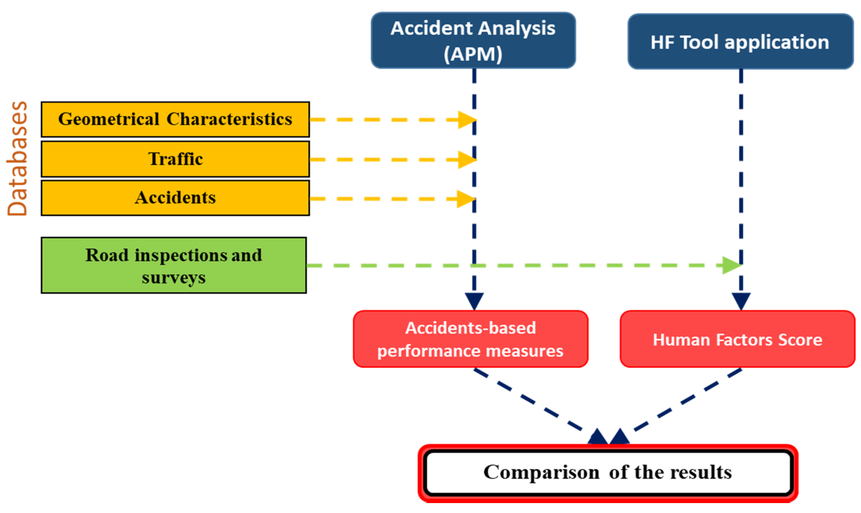
2. Materials and Methods
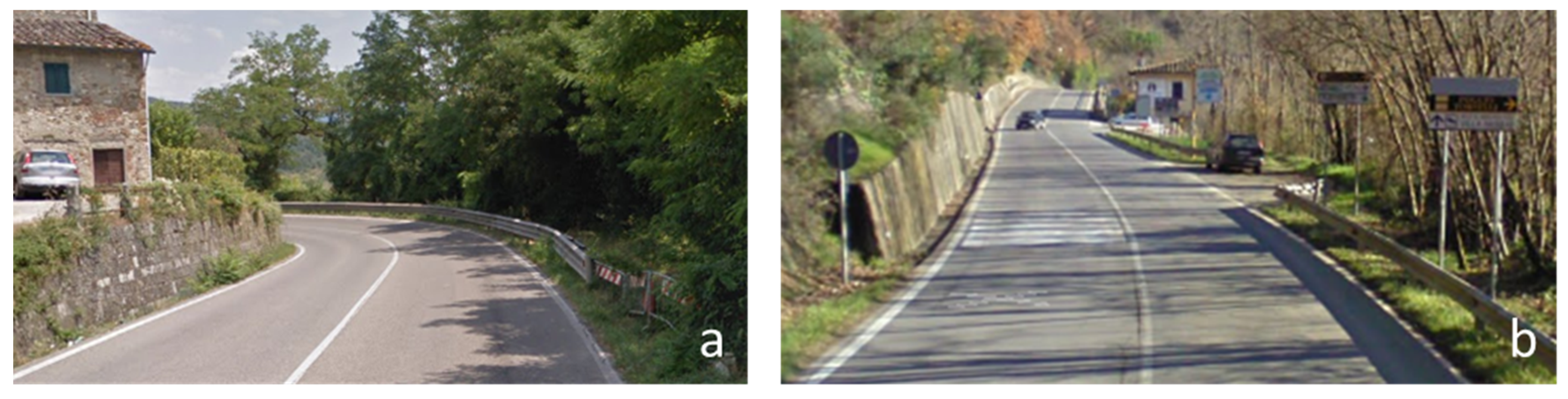
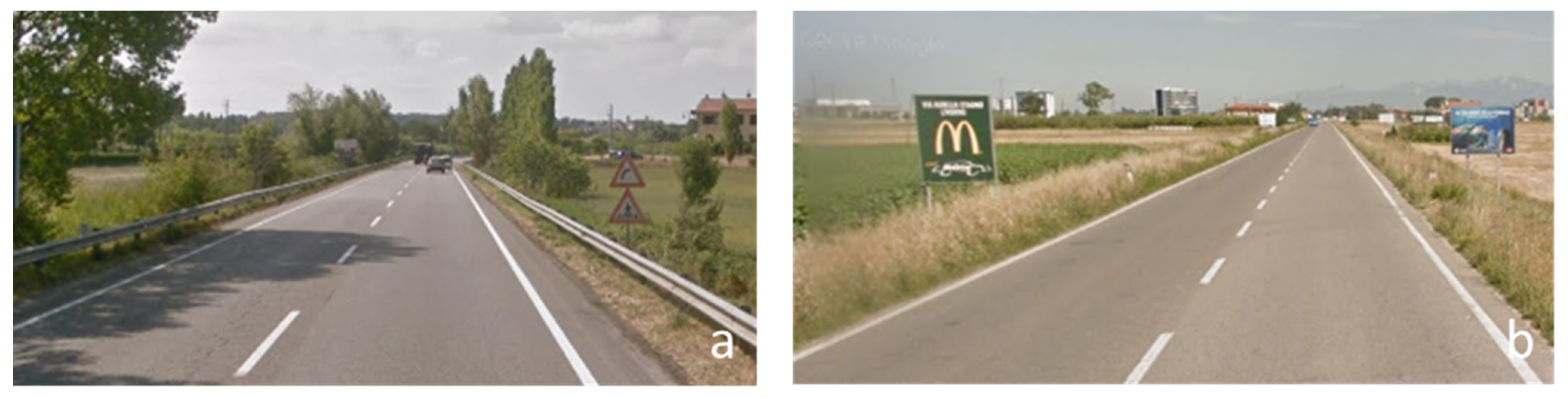
2.1. Test Roads

Two sections of two rural two-way two-lane roads, located in the Tuscan Region in Italy, were analyzed. These were the Strada Regionale 2 (SR2), from 281 + 600 km to 292 + 300 km, and the Strada Regionale 206 (SR206), from 29 + 600 km to 42 + 100 km. Figure 1 shows the two road stretches analyzed and their main geometrical features and differences.
The SR2 develops through a hilly stretch, characterized by many curves of a small radius, and it runs for a short stretch along the Greve river, maintaining a low curvature ratio. In the final part, the road passes through urban areas, reaching an important intersection junction with two roads of a higher functional class (two motorways). The road appears quite complex, with many curves of different radii and many driveways. The average carriageway width is 6.95 m, with no or very narrow shoulders and close marginal elements. Figure 2 shows two views of the SR2. The first shows a bend (on hilly terrain) that is difficult to understand because neither its curvature nor its development is clear; the second shows a picture taken about 90 m before an intersection that is quite invisible because the point of attraction is the top of the subsequent crest, and some marginal elements cover the minor road.
The SR206 develops in a flat environment and, overall, has a low curvature ratio, with a high presence of long straights and few intersections. The rural part of the road is generally clear and simple. The road passes through some small urban areas. There are many driveways along the road. The average carriageway width is 7.25 m, with 1 m paved shoulders on the central part of the road and very narrow paved shoulders on the remaining part. The left picture of Figure 3 shows a cross-section with shoulders of 1.5 m, while the one on right shows a cross-section with shoulders of about 0.5 m. The monotony of the margins is interrupted by some advertising panels, as shown in the right picture of Figure 3.

2.2. Procedure

The first activity concerned the segmentation process of the two considered test roads to subdivide them into homogeneous segments (HSs). According to the procedure described by PIARC [56], road safety inspections were performed for each homogeneous segment, and the Human Factors Score (HFS) was calculated. Finally, the HSM procedure was carried out, and each segment was assigned the expected number of accidents. The calculated HFS values and the accident-based performance measures of each segment were compared to assess their consistency. As shown in Figure 4, the HFET procedure requires less input data than the HSM analysis. Therefore, the procedure is also applicable in countries where a reliable accident, traffic, and geometrical database is not yet available.

2.3. Data Overview

Databases were provided by the Tuscan Region administration. They included the road characteristics, the traffic, and the accidents that occurred on the two test roads over 5 years (2014–2018). The road characteristics database considers a segmentation into segments with an average length of 100 m (ranging between 90 and 110 m). Each segment has an ID code, which refers to the name of the road and to the kilometers and hectometers markers they start from (e.g., the segment of SR2 starting from 234 + 300 km has the ID code SR2_234_3; the name of the road will be omitted if there is no risk of misunderstanding). The database contains the geometrical characteristics of each segment and specifies if they belong to the rural or urban environment. The segments and the location of each intersection were georeferenced.
The traffic database contains the traffic counts provided by inductive loops installed on the road network. In the test roads, there were four detection points: two on SR2 and two on SR206. The average traffic data along the considered road segments are shown in Table 1.
The accidents database was provided by the ISTAT (Italian National Statistical Board) and by the Tuscany Region Administration. It contains information about severe (fatal and injuries) accidents. The accidents were all georeferenced. The number of accidents, deaths, and injuries during the analysis period (2014–2018) is given in Table 1. No data about property-damage-only (PDO) accidents were available. All accidents caused by non-infrastructure-related problems were discarded; this translated into a total of two discarded accidents because they were caused by a vehicle breakdown. No accidents related to alcohol or drug abuse were in the database.

2.4. Test Roads Segmentation

The two test roads were subdivided into homogeneous segments (HSs) accounting for the road environment (urban and rural) and the type of road elements (roadway segments and intersections). The rural segments were divided into roadway segments and intersections segments. The urban segments were not divided. Each HS length ranged from 200 m to 1000 m. Their boundaries were rounded to fit the 100-meter-long segments of the available road characteristics database (see subchapter 2.3). The segmentation length was selected by accounting for the following factors:
  • accident triggering factors: these are located far away from the crash location reported in the crash reports, depending on speed and accident dynamics. Too-short road segments could be burdened by accidents that were caused by road deficiencies of a preceding road segment;
  • NSS management procedure: too-short road segments require high efforts in data collection and management. This has also been stated in the HSM [17], where the suggested minimum length is 0.1 mi (about 160 m);
  • critical segments identification: too-long segmentation will not help the identification of critical locations.
The influence length of an intersection was 75 m from the intersection geometrical center [59]. If adjacent intersections were closer than 250 m, then the HS included all close-spaced intersections and enclosed road segments. Adjacent Urban Segments were considered together. The segmentation process results are summarized in Table 2 and Table 3. A total of 47 HSs were obtained.
Figure 5 shows the traffic distribution along the two road stretches analyzed. The obtained segments are listed in the x-axis, while the corresponding traffic is depicted in the y-axis. SR2 has nearly half the traffic of SR206.

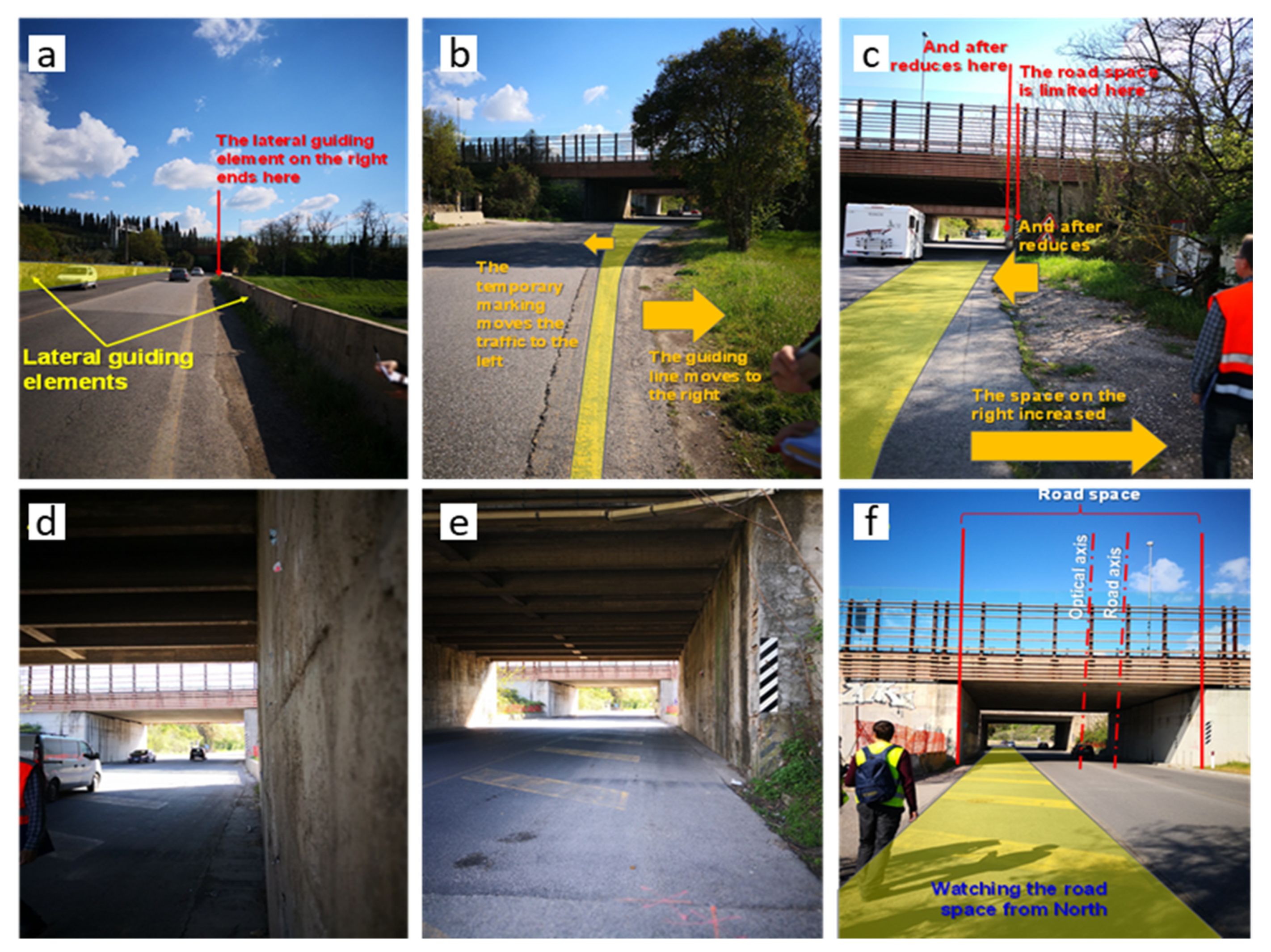
2.5. The Human Factors Evaluation Tool

The Human Factors Evaluation Tool is a road accident risk assessment tool developed by the researchers of Intelligenz System Transfer GmbH [58] and subsequently promoted and published by PIARC [56]. The tool allows for checking of the presence on the road of safety deficiencies non-compliant with the Human Factors rules. Namely, these are the 4–6 s rule (the road must provide enough time to see and read critical locations), the field of view rule (the road and its surrounding must provide a safe and clear field of view), and the logic rule (the road has to follow a driving logic) [39]. The HFET provides three checklists, one for each of the HF rules, to be filled out. Figure 6 presents an example of a checklist referring to the first HF rule, the 4–6 second rule. This specific checklist is divided into two sub-sections: 1st is “Moderation of transitional areas”, and 2nd is “Perception and visibility”. A critical point is a point on the road that forces the driver to change their driving program (a bend, an intersection, a bus stop, etc.). Column 1 of Figure 6 presents a list of questions referring to a Human Factor demand, i.e., a characteristic that the road should have to allow the correct driving performance in the specific road segment that is being analyzed. Each question should be answered as yes (score 1: the condition is present or satisfied) or no (score 0: the condition is not present, i.e., it is impossible to be analyzed or it is not met). The answer is noted in columns 5 and 6. Column 5 refers to the possible “fulfilment” of the condition (ACTUAL), if any. Column 6 (TARGET) represents the “presence” or the “desired presence” of the HF demand, depending on the considered road segment. Considering the example in Figure 6, point 2.1b means that the condition is required (target = 1) but not satisfied (actual = 0), while condition 2.2a is not required or it was impossible to analyze (target = 0 and actual = 0) (in this case, there were no curves in the HS). For each item, the worst condition along the inspected road segment was considered, and if a condition was only partially fulfilled, then 0 was annotated in the ACTUAL column. Once all the questions have been answered and the respective cells fulfilled, the HFS must be calculated for each sub-section of each checklist (in Figure 6: “Moderation of Transitional Area” and “Perception and Visibility”) and for the entire checklist (“4–6 s Rule Total” in Figure 6).
The HFS is calculated by summing up the values in the ACTUAL column and the TARGET column and calculating the ratio between ACTUAL and TARGET, as shown in Equation (1).
H F S = i = 1 n A C T U A L i i = 1 n T A R G E T i
where:
  • i = number of the considered condition
  • n = total number of conditions
  • ACTUAL = score in the “ACTUAL” column
  • TARGET = score in the “TARGET” column
Although only one calculation example for the First Rule is provided in this document, the calculation was done separately for each rule. Moreover, the calculation of the three rules together was also made (i.e., the Total HFS).
The comparison with the accident performance measures was made by considering the result of the Total HFS. The results allow one to classify the HS as having a low, medium, or high accident risk, based on the following criteria [56]:
  • Low risk: HFS > 60%
  • Medium risk: HFS > 40% but <60%
  • High risk: HFS < 40%
For each HS, the HFET evaluation sheets were filled, analyzing each HS through video recordings and notes that were taken during the road inspection. During the HFET application, some additional criteria were adopted to allow its application to segments that may comprise more than one critical point:
  • each homogeneous segment was analyzed in both directions; then, a merge of the results was made considering the worst results for each HF demand;
  • in processing the checklist of the first HF rule (4–6 s rule), the subsection 1 (“Moderation of transitional area” in Figure 6) was fulfilled for each identified critical point present in each HS, and the worst result was retained in the HFS calculation;
  • if one type of critical point was present several times along one segment (for instance, multiple curves), the worst result was taken.

2.6. The HSM Procedure and Accident-Based Performance Measures

The HSM procedure was applied using the IHSDM-HSM Predictive Method software®. All available data from each road were included in the model. Two models werebeen considered: the rural two-way two-lane model for the rural stretches of the road and the urban arterial model for the road stretches within the urban environment [17]. The following considerations were made:
  • a calibration factor was not available for the Urban arterial model; thus, the calibration factor was considered as 1;
  • the calibration factor for the rural two-way two-lane model was derived from the one by Martinelli et al. [59], and it was equal to 0.292;
  • the available road characteristics that were included in the calculation are shown in Table 4 (Rural: rural undivided two-lane highway; Urban: urban undivided two-lane arterial).
Two accident-based performance measures were chosen for the analysis. They were the accident frequency and the accident rate. These performance measures were then applied to the expected number of accidents obtained from the HSM procedure. They were calculated as follows:
  • Accident frequency (accidents/year): the frequency corresponds to the number of accidents per year in each HS, which is the expected number of accidents derived from the application of the HSM model.
  • Accident rate (accidents/(years*km*Mvehicles)): this corresponds to the accident density value divided by the value of the average annual traffic that affected the segment during the analysis period. Millions of vehicles (106 vehicles) are considered as traffic units. Equation (2) shows how the accident rate was calculated.
T = n L × 365 × ( A A D T m 10 6 )
where
  • T = accident rate (accidents/(years*km*Mvehicles));
  • n = yearly average number of accidents (accidents/year);
  • L = segment length (km);
  • AADTm = average between the average annual daily traffic value (AADT) of each year of the analysis period (vehicles/day).
The number of accidents considered in the two previous accident-performance measures is the result of applying the Empirical Bayes procedure to the HSM predictive model. The HSs safety levels, according to accident-based analysis, were defined considering the thresholds’ limits adopted by Tuscany Region Administration for the entire network [60]:
  • Tmean, which is the average of the values of an accident-based performance measure;
  • T80, which is the 80th percentile of the values of an accident-based performance measure; and
  • T90, which is the 90th percentile of the values of an accident-based performance measure.
The thresholds values considered are shown in Table 5. The given values are referred to the whole road network managed by the Tuscany Region administration and consider only the observed number of accidents. To compare the two approaches considered in the present study (accident-based approach and non-accident-based approach), the HSs werebeen classified as:
  • Low risk: performance measure < Tmean;
  • Medium risk: performance measure > Tmean and < T90;
  • High risk: performance measure > T90
This complies with the meaning of the threshold proposed by the Tuscany Region Administration.

2.7. Comparison

The results obtained from the application of the HFET and the accidents-based procedures were compared and discussed. The risk level classification and the HS ranking were compared. The relationship between the results was also tested using a linear correlation. A simple linear correlation was considered because the aim was to evaluate if a relationship exists between the results, not to investigate which function can best represent the relationship. The F-test was selected to consider the relationship between variances. The results wer tested considering a significance level of 5%. The correlation analysis was performed considering different data sets: a single dataset, which included the results of both the test roads (“Testing Group” 1—TG1); two distinct datasets, one for each test road (TG2); and three distinct datasets, one for each type of HS (i.e., Roadway Segments, Intersections Segments, and Urban Segments), regardless of the test road (TG3). Table 6 shows the composition of each Testing Group; the second column shows the total number of samples included in each group, while the other columns indicate the number of segments in the sample belonging to SR2 or SR206 and to each segment type, including both the roads.

3. Results

3.1. Human Factors Score

The HFS results of SR2 and SR206, deriving from the application of the HFET, are shown in Table 7 and Table 8. Table 7 shows the results for every single rule and the total result of the whole rule together, considering the worst results of both directions, as explained in subchapter 2.5. Table 8 shows the average results for each rule, each road, and each HS type. From the results in Table 7 and Table 8, the following can be inferred:
  • Most of the HSs of both the roads have a low score concerning the first rule, which means that the roads do not give enough time to detect, recognize, and correctly react to critical locations.
  • SR2 is characterized by the lowest HFS values, which means that there are more deficiencies concerning the HF demand. It includes two segments (282_9 and 291_0) ranked as highly risky. The most frequent deficiencies concern the first HF rule (40%).
  • SR206 has a higher score, confirming that its risk level is lower than SR2. The first HF rule is also the lowest in this case. No HS is of high risk.
  • The urban segments have the lowest mean score in all rules, which means they are the most dangerous ones from the HFS point of view.
  • Roadway segments present fewer safety problems than the intersection and the urban segment.
  • The third rule results are generally higher than or equal to the other results, except for Urban segments, where they are low. This complies with the more complex situation of the urban environment.
Considering the Human Factors-based approach, it emerged that SR2 has some important safety issues. SR2 presents many changes in the road environment, it includes critical locations that can surprise the driver, and its margins often change and are sometimes ambiguous. SR206 is a “simpler” road, with a long straight and a wide carriageway, where the different elements are clearer and more defined. SR206 has a long straight with a far longer depth of the field of view, but its geometrical monotony is partially compensated by a high number of elements along the margins, which improve the density of the peripheral view, disrupting the monotony and catching the attention of the driver closer to him (without distracting him).

3.2. Accident-Based Performance Measures

Table 9 shows the results obtained for the accident-based performance measures (i.e., accident frequency, accident density, and accident rate) derived from the application of the HSM procedure. The HSs are sorted by the value of the accident rate, including both road segments in a single list. The numbers included in the last three columns represent the ranking of each segment based on the value of each accident performance measure. Cell colors represent the level of risk according to the criteria defined in subchapter 2.7: the high risk is red, the medium risk is yellow, and the low risk is green. The thresholds of each risk level refer to the total value, not differentiated by HS type.
The results are also shown in Figure 7 by histograms. The results of SR2 are presented on the left side and SR206 on the right side. The thresholds Tmean and T90 are represented respectively with dashed green and red lines.
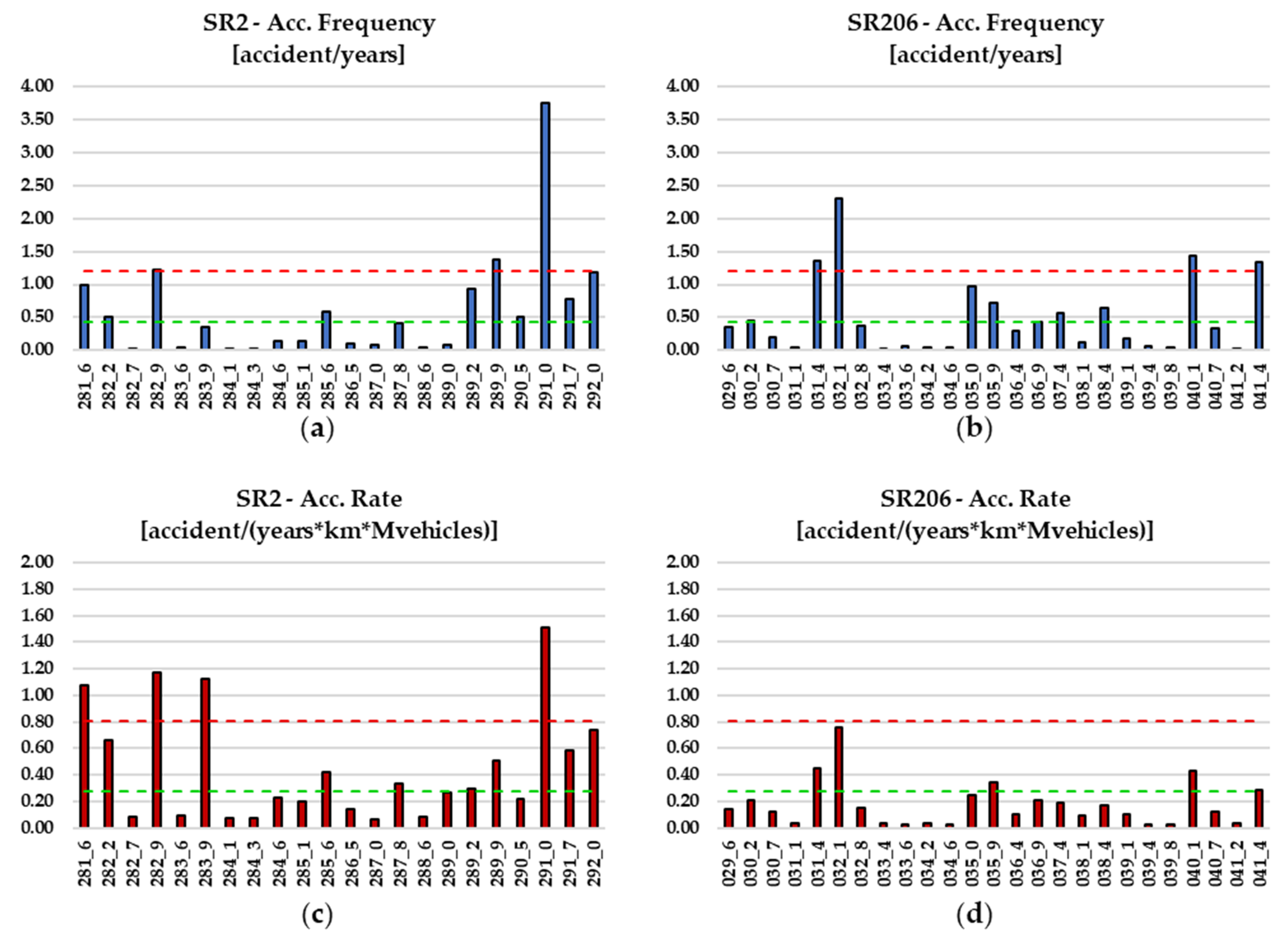
  • The two considered performance measures lead to different classifications. The exposure value (traffic and segment length) considerably changes the risk ranking. For instance, the segment SR2_283_9 was the third-most critical segment concerning the accident rate, but it was the 24th when considering the accident frequency. Similarly, SR206_032_1 was the second segment with the higher accident frequency value, but it was the fifth segment considering accident rate, passing from high risk to medium risk level.
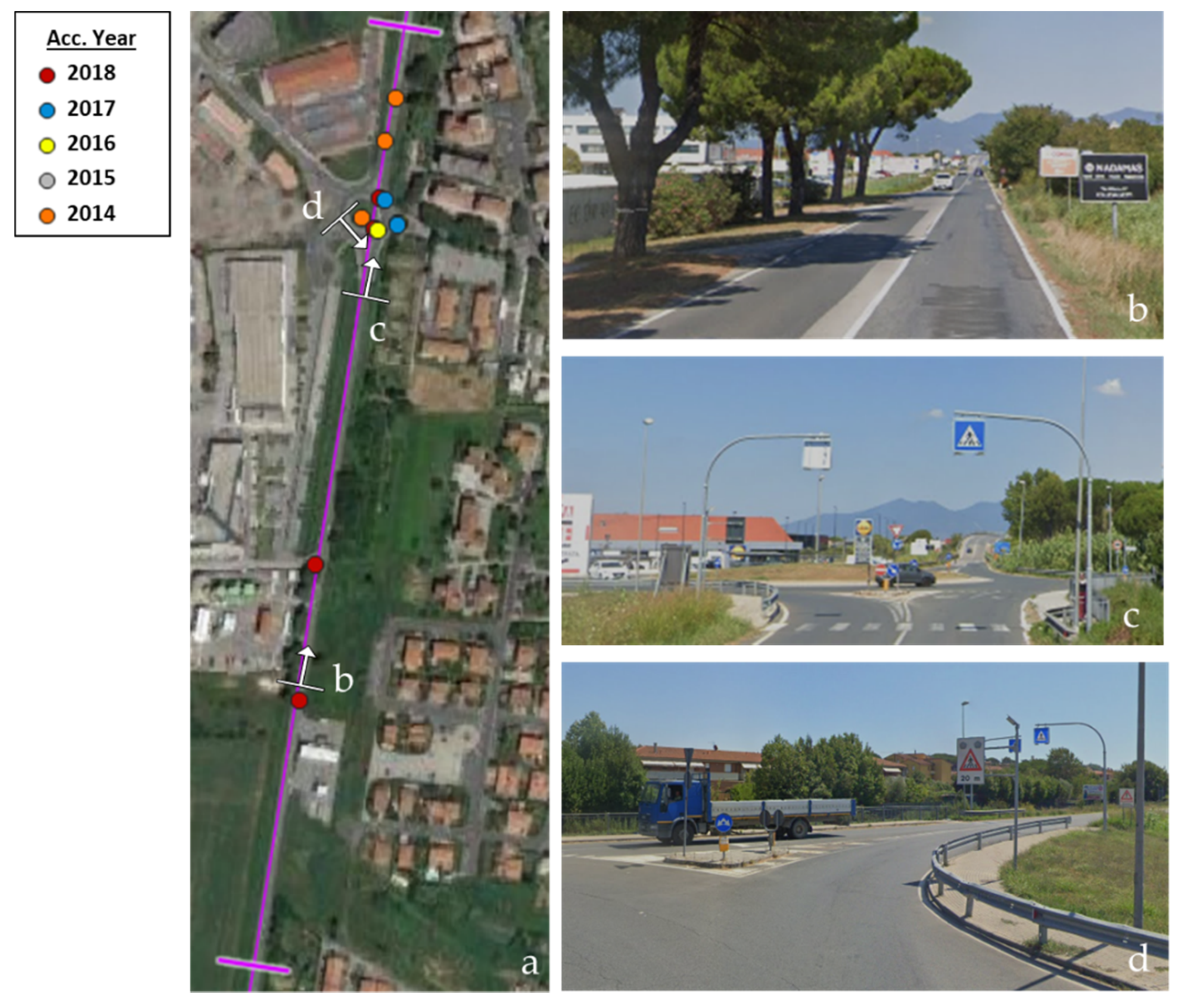
  • The most critical road was SR2. It had four segments above the T90 threshold for accident rate: 281_6, 282_9, 283_9, and 291_0. The first three were in the hilly terrain and included two narrow bends (first two) and a short segment with many driveways on a bend (SR2_283_9). The fourth was in the final part of the analyzed stretch. In this section, the AADT value was higher, and there was a mixture of urban and rural environments.
  • The SR206 has four segments (31_4, 32_1, 40_1, and 41_4) at high risk considering the accident frequency, while SR2 had only three segments over the T90 thresholds, which were 282_9, 289_9, and 291_0. The segments of SR206 generally “downgraded” to a lower risk if the accident rate was considered due to the higher traffic volume flowing through them.
  • An almost stable ranking was recorded for segments with a low risk of accidents; 26 segments were still low-risk segments for both the performance measures out of a total of 47 segments; six segments were still of medium risk level, and only two segments were still at a high-risk level. The low-risk level group of segments mostly included SR206 segments (16 for SR206 and 10 for SR2).
In conclusion, according to the results of the accident-based approach, SR2 had a high number of high-risk segments considering the accidents rate performance measure, but it was the opposite when considering the accident frequency. Because of the difference underlined in point “a.”, further on, to compare the results of the HFS and the accident-based methodologies, reference will be made only to the accident rate performance measure. The reason is that the accident rate is the performance measure that best fit the HFS, because they both focus only on the infrastructure in-built safety, regardless of exposure (once the index is fixed, the number of accidents will increase as the traffic increase).

3.3. Analysis and Comparison of the Results

Results from HFET implementation and accident-based analysis were compared and discussed. The overall results showed more critical conditions for SR2 than SR206.

3.3.1. Risk Level

The HFS and the accident rate results were compared in terms both of risk level and ranking. The ranking considered the two roads together. Table 10 shows the results, representing the risk level by colors and the respective ranking. The HSs are sorted in descending order based on the HFS results.
Table 10 makes it evident that the two approaches globally converge, giving the same response in many cases, but with some differences in the evaluation of the risk level. At the high-risk level, the HFS was more selective: only two HSs were judged as high risk, while the accident-based approach showed four critical segments. In both cases, the high-risk segments belonged to SR2. Fewer differences were found within the medium and low-risk levels, where the two approaches converged in 36 segments. Considering the risk level, 38 out of 47 segments (about 81%) were classified with the same risk level considering the HFS and the accidents rate results.
The most critical HS for both indices was the SR2_291_0, which is presented in Figure 8 and Figure 9. In Figure 8 an overview of the HS and the position of accidents that occurred in the segment are presented on a satellite image (picture a). Picture b, c, and d show three different photos taken along the segments. They represent the northbound approach to an intersection and the underpasses (b), the southbound approach to underpasses (c), and the point between the two underpasses southbound (d). A detailed sequence of pictures of the segment taken on the road is presented in Figure 9, considering the approach to underpasses southbound (from “a” to “e”) and a view of the underpasses northbound (f). The main issues identified are highlighted in the pictures. In this segment, 20 accidents occurred in the analysis period. The partial scores of the three HF rules were 19% for the First Rule, 42% for the Second Rule, and 39% for the Third Rule (see Table 7). There were several overlap problems in this segment. The main issue was represented by the intersection located immediately before an underpass in the north direction, which was completely invisible (picture b in Figure 8). Many side-collision accidents have occurred here. This explains the low score resulting from the First HF rule. Coming from North, two orientation problems occurred in sequence, in correspondence with the existing underpasses that were misaligned. The first one occurred when approaching the first underpass (pictures a, b, c of Figure 9).
The second most critical HS was the SR2_282_9, which was also ranked second in terms of accident rate, with eight observed accidents in the analysis period. On the left side of Figure 10, a representation of the segment on a satellite image is presented (a). On the right side of the same figure, three pictures are depicted of three critical points of the road southbound (b–d). In the middle of the segment, there is a sharp bend. The stretches preceding the bend from both directions are characterized by low curvature. In the central part of the bend, the shadow produced by the structure of an overpass hides the guidance element (safety barrier) on the external margin of the bend. Five out of eight accidents occurred on the bend, and these accidents were classified as head-on or side collisions. Two of these accidents were caused by drivers driving in the wrong direction and the rest by “distracted or indecisive driving”. This means that the driver could not clearly understand which trajectory they had to follow. The HFS resulted in 15% for the First Rule (the decision distance is missing), 39% for the Second Rule (the driver’s references in the field of view are lacking), and 44% for the Third Rule (the user does not expect the sharp bend) (the results are illustrated in Table 7).
These results underline that the HS has a serious problem of visibility, perception, and comprehension of the road and its elements. The stretches approaching the bend from both directions have a low curvature, thus drivers approach the sharp bend with an inappropriate speed. The bend’s curvature is not well-perceived because of the reduced visibility of lateral guidance. All these conditions can create confusion in drivers, wrong expectations, and underestimation of the risk. A great contribution to the score is given not only by the readability of the bend and its approaching segment, but also by the intersection, which is completely unexpected (see Figure 10—picture b).
In SR206, segment 032_1 is the most critical segment concerning the accident rate (the fifth when also considering SR2) and the sixth for HFS. In this segment, 14 accidents were observed in the analysis period. As Figure 11 shows, this HS is an Urban Segment, but the urban environment is unclear (houses are far away from the road margins, Figure 11—picture a).
There are driveways, intersections, and also pedestrian crossings (the road divides the residential area from the commercial area). The First Rule of the HF was the one with the lowest score (40%). This was mainly due to the poor visibility of driveways and crosswalks (Figure 11—pictures a and c). The HFS also highlighted some issues concerning the Third Rule (41%), which is the Logic Rule. The urban environment was not perceived, and also, the roundabout and its radius were not well perceived (Figure 11—pictures a and b), causing the driver to be surprised to find those elements.
The segment SR206_031_4 was ranked in the medium risk level for HF deficiencies but was burdened by fewer accidents (six accidents were observed in the analysis period). This HS has similar characteristics to the previous one and shows some problems both for the First and Third Rules of HF (50% and 51%, see Table 7). However, the HFS was higher, and the number of accidents was lower than the HS SR206_032_1. Figure 12 allows us to clarify this. It shows the approaching segment to the two roundabouts of SR206_031_4 (a) and SR206_032_1 (b).
The roundabout of SR206_031_4 is clearer and more perceivable. The road behind the roundabout is not visible, and the focal point approaching the roundabout is concentrated on the central island; the driver perceives the presence of the critical point (roundabout) in time and reduces the speed. In the roundabout of SR206_032_1, the driver’s attention is kept by the ascending segment of the road after the roundabout, and they do not concentrate on the roundabout itself, thus reducing to a lesser extent the speed and giving less attention to the vehicles engaging from the roundabout.
In conclusion, the two safety evaluation approaches converge in many cases, but each one presents peculiarity due to the different points of view from which the safety evaluation is done. A brief comment should be made to emphasize once again the proactive value of the HF procedure that analyses the current road situation.

3.3.2. Quantitative Relationship between HFS and Accident Rate

To investigate a trend correlation between the results, a comparison was made in terms of linear correlation, calculating the Pearson linear correlation coefficient, r, and testing its significance. The correlation was evaluated for the three groups of data (TG1–TG2–TG3), and the results are presented in Table 11. The table shows the testing group composition in the first two columns, the correlation coefficients r and R2 in columns 3 and 4, and, in the remaining columns, the significance level (α, column 5) and the F-test values (column 6 and 7). The test values’ column 6 shows the critical value for a significance of 5%, while column 7 shows the calculated actual value. If the actual value is higher than the critical value, the null hypothesis that the distribution occurred by chance can, thus, be rejected. Table 11 shows that for almost all sets, the actual value was higher than the critical value, and thus, the null hypothesis can be rejected. The only set where this condition did not occur was for Urban Segments (TG3). This was due to the quite dispersed distribution and the very low number of elements in the sample (only eight segments).
The results of r and R2 show that there was a correlation between the two variables, although it was not very strong. The objective of this analysis was not to produce a predictive model that exactly fitted the data but to demonstrate a correlation between the results and to prove that analyzing Human Factors aspects allows for the identifying dangerous locations.
Figure 13 illustrates the distribution of the HFS values vs the accident rate values for the TG1, including all the HSs of the two test roads together, and Figure 14 shows the HSs divided by road (TG2). The thresholds limits reported in the graphs refer to the total number of segments, not considering the segment type. The dashed green lines represent the thresholds between the medium- and low-risk segments, while the dashed red line represents the thresholds between the high- and medium-risk segments. Figure 13 and Figure 14 allow us to better understand the results of Table 11. There was an inverse relationship between the two variables: the lower the HFS was, the higher the accident rate was.
Finally, the relationship between HFS and accident rate was investigated, considering the different types of segments (roadway segments, intersections, and urban stretches, TG3). The results are presented in Figure 15. The threshold limits refer to the specific segments type, e.g., the T90 of an intersection was calculated considering only the segment type “intersection” within the Tuscan Region network. Urban segments were characterized by fewer data. Furthermore, no specific calibration factor for the urban arterial was available. For these reasons, the Urban segment’s result could not be representative.
Looking at the results in Figure 15, a better relationship occurred for Intersections segments rather than Road segments or Urban segments. Furthermore, moving from Roadway segments, which are less complex types of segments (in terms of conflict points and road users flow), to Intersections and Urban segments (more complex segment types) the slope of the linear regression line increased. The conflict probabilities increased in the latter situations, and the number of accidents increased consequently. The general trend found in TG1 and TG2 was confirmed. Thus, it seems that the methodology allowed for identifying of critical segments with enough reliability.
Better results could be obtained if an accident database was available that included all accidents occurring on the road section considered, including those that resulted in property damage only (PDO). The wrong stimuli provided by a low self-explaining road (i.e., a road that does not satisfy the HF demands) can give rise to both serious accidents and PDO accidents. Accidents’ severity is due to the passive safety of the road and accident randomness. The latter is due to the overlapping of random events and an accident’s dynamic (variation of speed at the impact and type of collision). Therefore, a statistical relationship based on a more substantial dataset, including both serious and PDO accidents, should be investigated.

4. Conclusions

Identifying hazardous segments, considering how the road is perceived by drivers, is a fairly new way of analysis. It is not the driver who does not comply with the road but the road that provides misguiding information. The inclusion of these aspects in NSSs allows one to considerably improve the effectiveness of the procedure. Moreover, analyzing road safety by employing proactive procedures means not waiting for accidents to occur.
The paper analyzed the effectiveness of a proactive road safety analysis procedure suitable for NSSs, which was based on the analysis of Human Factors aspects. The proposed procedure was based on the use of the HFET proposed by PIARC [56]. The HFET belongs to a proactive investigation methodology that allows for analyzing of the safety performance of a road segment in terms of interaction between the driver and the road environment. The effectiveness of the procedure was tested by comparing the results from the HFET analysis to those of a standard reactive procedure. The latter was based on the application of the HSM predictive model for rural two-lane two-way roads, adjusted for the observed number of accidents using the EB methodology. Both the procedures were applied to two rural two-lane two-way road stretches, for a total length of 23 km.
The outputs of the procedures were compared in terms of risk level and linear correlation. A good correspondence was found in the evaluation. About 81% of the total number of segments analyzed were classified with the same level of risk for both procedures. The linear correlation between the two variables was not strong; thus, a linear function could not clearly explain the relationship between the two variables. However, an inverse relation was present. Overall, the relationship found confirmed the coherence of the two performance measures. Thus, the used methodology seems able to identify critical road sections.
Some strengths and weaknesses were also found. Adopting a safety screening based on the proposed HFET procedure offers multiple advantages:
  • it is a proactive procedure;
  • it allows for implementing of NSS, even if reliable accident databases are not available, as mainly occurs in low- and medium-income countries.
On the other hand, one of the main weaknesses of this procedure is that it requires time to be carried out; this may limit its use from RAs. Moreover, the study considered only fatal and injury accidents, and the HFET checklists should be improved in structure and format to be easily applicable.
Consequently, further research should focus on how to reduce the application time and the usability of the HFET. Moreover, the research should be improved by including in the analysis both the severe accidents (as done in the performed study) and the PDO accidents. For further developments, a comprehensive analysis is recommended, considering more roads and including both severe and PDO accidents.

Author Contributions

Conceptualization, A.P. and L.D.; methodology, A.P., L.D., M.M. and V.B.; validation, A.P., L.D., M.M. and V.B.; formal analysis, L.D.; investigation, A.P. and L.D.; resources, A.P., M.M. and V.B.; data curation, A.P., M.M. and V.B.; writing—original draft preparation, A.P.; writing—review and editing, A.P., L.D., M.M. and V.B.; visualization, A.P., L.D., M.M. and V.B.; supervision, L.D.; project administration, L.D.; funding acquisition, L.D., M.M. and V.B. All authors have read and agreed to the published version of the manuscript.

Funding

This research is part of the research project of CMRSS “Attuazione progetto del Centro di Monitoraggio della Sicurezza Stradale della Regione Toscana (2° programma attuativo del piano nazionale della sicurezza stradale)—Sezione studi e ricerche: attività di ricerca finalizzata in via principale alla definizione di elementi scientifici di supporto ad un metodo per la gestione in sicurezza delle strade non appartenenti alla rete TEN, come supporto degli adempimenti Regionali di cui all’art.1, comma 4, del d.lgs. N°35/2011”, funded by the Tuscan Region administration.

Institutional Review Board Statement

Not applicable.

Informed Consent Statement

Not applicable.

Data Availability Statement

The datasets used in this study were provided by Tuscan Region and ISTAT under the agreement “File di metadata per la ricerca—MFR (Microdata for Research)”. The data are not publicly available due to a Non-Disclosure Agreement.

Conflicts of Interest

The authors declare no conflict of interest.

References

  1. WHO. Global Status Report on Road Safety 2018; WHO: Geneva, Switzerland, 2019. [Google Scholar]
  2. European Transport Safety Council. BRIEFING—EU Strategic Action Plan on Road Safety; European Transport Safety Council: Brussels, Belgium, 2019. [Google Scholar]
  3. European Parliament. Directive 2008/96/EC of the European Parliament and of the Council of 19 November 2008 on Road Infrastructure Safety Management. Off. J. Eur. Union 2008, 50, 59–67.
  4. UNECE. Road Safety Audit and Road Safety Inspection on the TEM Network; United Nations Economic Commission for Europe: Geneva, Switzerland, 2018. [Google Scholar]
  5. PIARC. Road Safety Manual. 20 October 2019. Available online: https://roadsafety.piarc.org/en (accessed on 5 August 2021).
  6. ITF. Zero Road Deaths and Serious Injuries: Leading a Paradigm Shift to a Safe System; OECD Publishing: Paris, France, 2016. [Google Scholar]
  7. Srinivasan, R.; Gross, F.; Lan, B.; Bahar, G. Reliability of Safety Management Methods: Network Screening; U.S. Department of Transportation—Federal Highway Administration: Washington, DC, USA, 2016.
  8. Ghadi, M.; Török, Á. Comparison different black spot identification methods. Transp. Res. Procedia 2017, 27, 1105–1112. [Google Scholar] [CrossRef]
  9. Heydari, S.; Hickford, A.; McIlory, R.; Turner, J.; Bachani, A.M. Road safety in low-income countries: State of the knowledge and future directions. Sustainability 2019, 11, 6249. [Google Scholar] [CrossRef] [Green Version]
  10. Yannis, G.; Dragomanovits, A.; Laiou, A.; Ritcher, T.; Ruhl, S.; Torre, F.L.; Domenichini, L.; Graham, D.; Karathodorou, N.; Li, H. Use of accident prediction models in road safety management—An international inquiry. In Proceedings of the 6th Transport Research Arena (TRA 2016), Warsaw, Poland, 18–21 April 2016. [Google Scholar]
  11. Greibe, P. Accidents prediction model for urban roads. Accid. Anal. Prev. 2003, 35, 273–285. [Google Scholar] [CrossRef]
  12. Cafiso, S.; Di Graziano, A.; Di Silvestro, G.; La Cava, G. Development of comprehensive accident models for two-lane rural highways using exposure, geometry, consistency and context variables. Accid. Anal. Prev. 2010, 42, 1072–1079. [Google Scholar] [CrossRef] [PubMed]
  13. Moraldi, F.; La Torre, F.; Ruhl, S. Transfer of the highway safety manual predictive method to German rural two-lane, two-way roads. J. Transp. Saf. Secur. 2020, 12, 977–996. [Google Scholar] [CrossRef]
  14. La Torre, F.; Meocci, M.; Nocentini, A. Safety effects of automated section speed control on the Italian motorway network. J. Saf. Res. 2019, 69, 115–123. [Google Scholar] [CrossRef]
  15. Montella, A.; Mauriello, F. Procedure for ranking unsignalized intersections for safety improvement. Transp. Res. Board 2012, 2318, 75–82. [Google Scholar] [CrossRef]
  16. Šenk, P.; Ambros, J.; Pokorný, P.; Striegler, R. Use of accident prediction models in identifying hazardous road locations. Trans. Transp. Sci. 2012, 5, 223–232. [Google Scholar] [CrossRef] [Green Version]
  17. American Association of State and Highways Transportation Official. HSM—Highway Safety Manual, 1st ed.; American Association of State and Highways Transportation Official: Washington, DC, USA, 2010. [Google Scholar]
  18. American Association of State and Highways Transportation Official. Highway Safety Manual 2014 Supplement; American Association of State and Highways Transportation Official: Washington, DC, USA, 2014. [Google Scholar]
  19. La Torre, F.; Domenichini, L.; Meocci, M.; Graham, D.; Karathodorou, N.; Richter, T.; Ruhl, S.; Yannis, G.; Dragomanovits, A.; Laiou, A. Development of a transnational accident prediction model. In Proceedings of the 6th Transport Research Arena (TRA 2016), Warsaw, Poland, 18–21 April 2016. [Google Scholar]
  20. La Torre, F.; Meocci, M.; Domenichini, L.; Branzi, V.; Tanzi, N.; Paliotto, A. Development of an accident prediction model for Italian freeways. Accid. Anal. Prev. 2019, 124, 1–11. [Google Scholar] [CrossRef] [PubMed]
  21. Wan, Y.; He, W.; Zhou, J. Urban road accident black spot identification and classification approach: A novel grey verhuls–Empirical bayesian combination method. Sustainability 2021, 13, 11198. [Google Scholar] [CrossRef]
  22. Yuan, Q.; Xu, X.; Xu, M.; Zhao, J.; Li, Y. The role of striking and struck vehicles in side crashes between vehicles: Bayesian bivariate probit analysis in China. Accid. Anal. Prev. 2020, 134, 105324. [Google Scholar] [CrossRef] [PubMed]
  23. PIARC. Accidents Investigations Guidelines for Road Engineers; PIARC: Paris, France, 2013; ISBN 978-2-84060-321-4. [Google Scholar]
  24. Treat, J.R.; Tumbas, N.S.; McDonald, S.T.; Shinar, D.; Hume, R.D.; Mayer, R.E.; Stansifer, R.L.; Castellan, N.J. Tri-Level Study of the Causes of Traffic Crashes: Final Report—Executive Summary; Report No. DOT-HS-034-3-535-79-TAC(S); Institute for Research in Public Safety: Bloomington, IN, USA, 1979. [Google Scholar]
  25. National Cooperative Highway Research Program (NCHRP). Human Factors Guidelines, 2nd ed.; Transport Research Board—Report 600; National Cooperative Highway Research Program (NCHRP): Washington, DC, USA, 2012; ISBN 978-0-309-25816-6. [Google Scholar]
  26. Shinar, D.; Rockwell, T.; Malecki, J. The effects of changes in driver perception on rural curve negotiation. Ergonomics 1980, 23, 263–275. [Google Scholar] [CrossRef]
  27. Perco, P. Desirable length of spiral curves for two-lane rural roads. J. Transp. Res. Board 2006, 1961, 1–8. [Google Scholar] [CrossRef]
  28. McGee, H.; Moore, W.; Knapp, B.; Sanders, J. Decision Sight Distance for Highway Design and Traffic Control Requirements; (FHWA-RD-78-78); Department of Transportation: Washington, DC, USA, 1978.
  29. Intini, P.; Berloco, N.; Colonna, P.; Ranieri, V.; Ryeng, E. Exploring the relationships between drivers’ familiarity and two-lane rural road accidents—A multi-level study. Accid. Anal. Prev. 2018, 111, 280–296. [Google Scholar] [CrossRef]
  30. Yanko, M.R.; Spalek, T.N. Route familiarity breeds inattention: A driving simulator study. Accid. Anal. Prev. 2013, 57, 80–86. [Google Scholar] [CrossRef]
  31. Domenichini, L.; La Torre, F.; Branzi, V.; Nocentini, A. Speed behaviour in work zone crossovers—A driving simulator study. Accid. Anal. Prev. 2017, 98, 10–24. [Google Scholar] [CrossRef]
  32. Ben-Bassat, T.; Shinarb, D. Effect of shoulder width, guardrail and roadway geometry on driver perception and behaviour. Accid. Anal. Prev. 2011, 43, 2142–2152. [Google Scholar] [CrossRef]
  33. Montella, A.; Aria, M.; D’Ambrosio, A.; Galante, F.; Mauriello, F.; Pernetti, M. Simulator evaluation of drivers’ speed, deceleration and lateral position at rural intersections in relation to different perceptual cues. Accid. Anal. Prev. 2011, 43, 2072–2084. [Google Scholar] [CrossRef]
  34. Domenichini, L.; Branzi, V.; Meocci, M. Virtual testing of speed reduction schemes on urban collector roads. Accid. Anal. Prev. 2018, 110, 38–51. [Google Scholar] [CrossRef]
  35. Branzi, V.; Meocci, M.; Domenichini, L.; La Torre, F. Drivers’ performance in response to engineering treatments at pedestrian crossings. Adv. Transp. Stud. 2018, 1, 55–70. [Google Scholar] [CrossRef]
  36. Bassani, M.; Sacchi, E. Calibration to local conditions of geometry-based operating speed models for urban arterials and collectors. Procedia Soc. Behav. Sci. 2012, 53, 822–833. [Google Scholar] [CrossRef] [Green Version]
  37. Recarte, M.A.; Nunes, L.M. Mental workload while driving: Effects on visual search, discrimination, and decision making. J. Exp. Psychol. Appl. 2003, 9, 119–137. [Google Scholar] [CrossRef]
  38. Jovanović, D.; Šraml, M.; Matović, B.; Mićić, S. An examination of the construct and predictive validity of the self-reported speeding behavior model. Accid. Anal. Prev. 2017, 99, 66–76. [Google Scholar] [CrossRef] [PubMed]
  39. PIARC. Human Factors Guidelines for a Safer Man-Road Interface; PIARC Publications: Paris, France, 2016. [Google Scholar]
  40. RoSPA. Social Factors in Road Safety—Policy Paper; The Royal Society for the Prevention of Accidents (RoSPA): Birmingham, UK, 2012. [Google Scholar]
  41. González-Sánchez, G.; Olmo-Sánchez, M.I.; Maeso-González, E.; Gutiérrez-Bedmar, M.; García-Rodríguez, A. Traffic injury risk based on mobility patterns by gender, age. Sustainability 2021, 13, 10112. [Google Scholar] [CrossRef]
  42. Wu, Y.; Boyle, L.; McGehee, D.; Roe, C.A.; Kazutoshi, E.; James, F. Modeling types of pedal applications using a driving simulator. J. Hum. Factors Ergonom. Soc. 2015, 57, 1276–1288. [Google Scholar] [CrossRef]
  43. Theeuwes, J. Sampling information from the road environment. In Human Factors for Highway Engineers; Pergamon: New York, NY, USA, 2002; pp. 131–146. [Google Scholar]
  44. Theeuwes, J. Self-explaining roads and traffic system. In Designing Safe Road Systems: A Human Factors Perspective; CRC Press: New York, NY, USA, 2012; pp. 11–26. [Google Scholar]
  45. Theeuwes, J.; Godthelp, H. Self-explaining roads. Saf. Sci. 1995, 19, 217–225. [Google Scholar] [CrossRef]
  46. Godthelp, J. Traffic safety in emerging countries: Making roads self-explaining through intelligent support systems. In Proceedings of the 26th World Road Congress, Abu Dhabi, United Arab Emirates, 6–10 October 2019. [Google Scholar]
  47. Theeuwes, J. Self-explaining roads: What does visual cognition tell us about designing safer roads? Cogn. Res. Princ. Implic. 2021, 6, 15. [Google Scholar] [CrossRef]
  48. Qin, Y.; Chen, Y.; Lin, K. Quantifying the effects of visual road information on drivers’ speed choices to promote self-explaining roads. Int. J. Environ. Res. Public Health 2020, 17, 2437. [Google Scholar] [CrossRef] [Green Version]
  49. Köhler, W. Evoluzione e Compiti della Psicologia della Forma; Armando Editore: Rome, Italy, 2008; p. 25. ISBN 978-88-6081-356-5. [Google Scholar]
  50. Birth, S. Human factors design features supporting space perception. In Proceedings of the 4th International Conference on Safer Road Infrastructure, Prague, Czech Republic, 14–17 April 2009. [Google Scholar]
  51. Birth, S.; Demgensky, B.; Aubin, D. Space Perception and Road Design for Vulnerable Road User; PIARC: Paris, France, 2009. [Google Scholar]
  52. Birth, S.; Staadt, H.; Sporbeck, O. Guideline for Optical Orientation by Planting, (HVO); Ministry of Infrastructure and Regional Development: Postdam, Germany, 2002.
  53. Čičković, M. Influence of human behaviour on geometric road design. In Proceedings of the 6th Transport Research Arena (TRA 2016), Warsaw, Poland, 18–21 April 2016; pp. 4364–4373. [Google Scholar]
  54. Birth, S.; Demgensky, B.; Sieber, G. Relationship between Human Factors and the Likelihood of Single-Vehicle Crashes on Dutch Motorways; Report for Rijkswaterstaat Dienst Verkeer en Scheepvaart; PIARC: Delft, The Netherlands, 2015. [Google Scholar]
  55. Birth, S.; Demgensky, B. Investigation of Human Factors Accident Triggers on Rural Roads in Brandeburg, Germany; Ministry of Infrastructure and Regional Development: Postdam, Germany, 2017.
  56. PIARC. Road Safety Evaluation Based on Human Factors Method; World Road Association; PIARC: Paris, France, 2018. [Google Scholar]
  57. Birth, S.; Pflaumbaum, M. Human factors in road design: A way to self-explaining roads; Validation of the IST-Checklist 2005, Project Report of Work Package 3: Expert assistance for safety review of rural and urban roads (single carriageway roads). In Ranking for European Road Safety (RANKERS) Research Project Funded under the 6th Framework Program of the European Community; European Commission: Brussels, Belgium, 2006. [Google Scholar]
  58. Birth, S.; Demgensky, B.; Sieber, G. Human Factors Evaluation Tool; Intelligenz System Transfer GmbH: Postdam, Germany, 2017. [Google Scholar]
  59. Martinelli, F.; La Torre, F.; Vadi, P. Calibration of the Highway Safety Manual’s Accident Prediction Model for Italian Secondary Road Network. J. Transp. Res. Board 2009, 2103, 1–9. [Google Scholar] [CrossRef]
  60. Regione Toscana. Analisi di Incidentalità delle Strade Regionali; Centro di Monitoraggio Regionale—Direzione Politiche Mobilità, Infrastrutture e TPL—Settore Programmazione Viabilità: Florence, Italy, 2019. [Google Scholar]
Figure 1. The two analyzed road segments: SR2 (a) and SR206 (b). The Kilometers markers direction is northbound for both the roads.
Sustainability 14 00662 g001
Figure 2. Photos of SR2: 282 + 100 km northbound (a), and 288 + 400 km southbound (b).
Sustainability 14 00662 g002
Figure 3. Photos of SR206: 33 + 700 km southbound (a), and 39 + 200 km northbound (b).
Sustainability 14 00662 g003
Figure 4. Flow chart of the required data and steps implemented in the analysis.
Sustainability 14 00662 g004
Figure 5. Traffic volume distribution for each HS for SR2 (a) and for SR206 (b).
Sustainability 14 00662 g005
Figure 6. Example of HFET sheet fulfilment.
Sustainability 14 00662 g006
Figure 7. Histogram of the results for each HS, for SR2 accident frequency (a), SR206 accident frequency (b), SR2 accident rate (c), and SR206 accident rate (d).
Sustainability 14 00662 g007
Figure 8. SR2_291_0 HS with accidents’ locations on a satellite image (a) and two pictures of the HS in the northbound direction (b) and one in the southbound direction (c,d).
Sustainability 14 00662 g008
Figure 9. A sequence of pictures approaching the overpasses northbound (ae) and one picture taken southbound (f).
Sustainability 14 00662 g009
Figure 10. SR2_282_9 HS with accidents’ locations on a satellite image (a) and three pictures of the HS in the southbound direction (bd).
Sustainability 14 00662 g010
Figure 11. SR206_032_1 HS with accidents’ location on a satellite image (a) and two pictures of the HS in the northbound direction (b,c), and one in the southbound direction, exiting the roundabout (d).
Sustainability 14 00662 g011
Figure 12. Approach to roundabout: SR206_031_4 (a) and SR206_032_1 (b).
Sustainability 14 00662 g012
Figure 13. Correlations between HFS and accident rate for TG1.
Sustainability 14 00662 g013
Figure 14. Correlations between HFS and accident rate for TG2. The results are presented for SR2 (a) and SR206 (b).
Sustainability 14 00662 g014
Figure 15. Correlations between HFS and accident rate for TG3. The results are presented for Roadway Segments (a), Intersections Segments (b), and Urban Segments (c).
Sustainability 14 00662 g015
Table 1. Overall accidents and traffic parameters of the analyzed road segments.
RoadAnalyzed
Segment Length [km]
Mean Average AADT 1
[Veh/Days]
Max Average AADT 1
[Veh/Days]
Min Average AADT 1
[Veh/Days]
Total
Accidents
Fatal
Accidents
Injury
Accidents
SR210.41646912,395424783182
SR20612.7512,93115,33511,79978177
1 Considering the mean/max/min of the average AADT of all segments. Average AADT is calculated as the average of the segment AADT in the analysis period.
Table 2. Main characteristics of the HSs.
TypeMaximum Length [m]Minimum Length [m]Average Length [m]
Roadway Segments (rural)908200490
Intersections (rural)903190498
Urban Segments707296599
Table 3. HSs obtained for each road.
SR2
Section IDLength [km]Section Type
281_60.60Roadway Segment
282_20.50Intersections
282_70.20Roadway Segment
282_90.68Intersections
283_60.29Roadway Segment
283_90.20Intersections
284_10.22Roadway Segment
284_30.22Intersections
284_60.43Roadway Segment
285_10.50Intersections
285_60.91Roadway Segment
286_50.51Intersections
287_00.81Roadway Segment
287_80.80Intersections
288_60.40Roadway Segment
289_00.20Intersections
289_20.70Urban Segment
289_90.60Urban Segment
290_50.50Urban Segment
291_00.55Intersections
291_70.30Urban Segment
292_00.35Intersections
SR206
Section IDLength [km]Section Type
029_60.60Intersections
030_20.50Roadway Segment
030_70.40Intersections
031_10.30Roadway Segment
031_40.70Urban Segment
032_10.71Urban Segment
032_80.58Urban Segment
033_40.19Intersections
033_60.58Roadway Segment
034_20.39Intersections
034_60.39Roadway Segment
035_00.90Intersections
035_90.49Roadway Segment
036_40.69Intersections
036_90.49Intersections
037_40.69Roadway Segment
038_10.30Intersections
038_40.70Urban Segment
039_10.30Roadway Segment
039_40.40Intersections
039_80.30Roadway Segment
040_10.60Intersections
040_70.50Intersections
041_20.20Roadway Segment
041_40.82Intersections
Table 4. Available road characteristics included in the model.
CharacteristicsRuralUrban
Horizontal element start locationXX
Horizontal element end locationXX
Curve radiusXX
Curve directionXX
Curve side of the roadXX
Vertical element start locationXX
Vertical element end locationXX
GradeXX
Lane widthXX
Overtaking maneuver allowedXX
Shoulder widthXX
Shoulder typeXX
Design speedX
Driveway densityX
Roadside hazard ratingX
LightingXX
Automated speed enforcementXX
Presence of centerline rumble stripX
Presence of median X
Presence of median barrier X
Posted speed X
Speed category X
Number of driveways X
Type of driveway X
Presence of rail highway crossing X
On-street parking X
Table 5. Accident-based performance measures thresholds based on the Tuscany Region network.
Acc. Frequency
[Acc./Years]
Acc. Rate
[Acc./(Years*km*Mvehicles)]
Segment Type Tmean T80 T90 Tmean T80 T90
Roadway0.160.200.400.160.280.46
Intersections0.300.400.800.300.530.88
Urban1.252.203.200.500.821.09
Total0.440.601.200.280.480.81
Table 6. Composition of the Testing Groups.
Testing GroupsSamples
Total (n)RoadHomogeneous Segment Type
SR2SR206RoadwayIntersectionsUrban
TG147222517228
TG22222-8104
25-259124
TG3178917--
221012-22-
844--8
Table 7. HFS results for each rule, considering both the directions together.
SR 2SR206
1234512345
H.S. NameHFS
I Rule
HFS
II Rule
HFS
III Rule
HFS
Total
H.S. NameHFS
I Rule
HFS
II Rule
HFS
III Rule
HFS
Total
281_630%41%71%48%029_664%76%76%73%
282_238%68%65%59%030_257%81%77%73%
282_780%79%90%82%030_775%82%87%83%
282_915%39%44%36%031_150%82%73%71%
283_630%71%72%67%031_450%67%52%57%
283_925%55%47%47%032_140%56%41%45%
284_180%84%89%85%032_844%65%65%58%
284_356%71%81%72%033_458%90%72%76%
284_650%67%79%68%033_640%87%79%72%
285_154%41%72%53%034_277%88%75%80%
285_631%54%52%48%034_6100%89%78%90%
286_554%58%68%61%035_024%52%44%42%
287_044%60%74%61%035_940%68%75%62%
287_815%67%50%48%036_450%69%63%62%
288_615%71%61%54%036_940%72%50%57%
289_040%83%65%68%037_440%63%75%62%
289_231%58%38%44%038_140%65%80%64%
289_933%63%59%53%038_433%72%57%58%
290_538%79%61%62%039_1100%73%90%81%
291_019%42%39%34%039_460%63%81%69%
291_738%47%52%47%039_8100%73%90%82%
292_015%50%57%45%040_140%50%43%45%
040_744%64%80%66%
041_290%80%87%84%
041_438%64%55%54%
Table 8. Average HFS for each rule.
First
HF Rule
Second
HF Rule
Third
HF Rule
All
HF Rules
Total HSs48%67%67%62%
SR240%62%64%58%
SR20656%72%70%67%
Roadway58%72%78%70%
Intersection44%65%65%60%
Urban39%63%53%53%
Table 9. Performance measures results, ranking, and risk level.
RoadHS NameAcc. Frequency
[Acc./y]
Acc. Rate
[Acc./(km*Mveh)]
# Acc.
Frequency
# Acc.
Rate
SR2291_03.751.5111
SR2282_91.231.1772
SR2283_90.351.13243
SR2281_61.001.0894
SR206032_12.300.7625
SR2292_01.190.7486
SR2282_20.520.66177
SR2291_70.790.59128
SR2289_91.390.5149
SR206031_41.350.45510
SR206040_11.430.43311
SR2285_60.590.421512
SR206035_90.730.341313
SR2287_80.410.332114
SR2289_20.930.291115
SR206041_41.340.29616
SR2289_00.080.273317
SR206035_00.970.251018
SR2284_60.150.223019
SR2290_50.500.221820
SR206030_20.450.211921
SR206036_90.440.212022
SR2285_10.150.192923
SR206037_40.570.191624
SR206038_40.650.171425
SR206032_80.370.152226
SR2286_50.110.143227
SR206029_60.360.142328
SR206030_70.210.122729
SR206040_70.330.122530
SR206039_10.180.102831
SR206036_40.300.102632
SR2283_60.040.094133
SR206038_10.120.093134
SR2288_60.050.083935
SR2282_70.020.084736
SR2284_30.030.074537
SR2284_10.020.074638
SR2287_00.080.063439
SR206033_40.030.044440
SR206041_20.040.034341
SR206031_10.040.034242
SR206034_20.050.033743
SR206034_60.050.033844
SR206033_60.070.033545
SR206039_80.040.034046
SR206039_40.060.033647
Table 10. Comparison of the risk level classification based on accident rate (all types) and HF.
SR2SR206
HS IDAcc. RateHFSHS IDAcc. RateHFS
291_011035_0183
282_922032_156
289_2154040_1117
292_065041_41615
283_938031_41018
291_789036_92217
285_61210038_42519
287_81411032_82620
281_6412035_91324
289_9913037_42425
285_12314036_43227
288_63516038_13429
282_2721040_73030
286_52722039_44733
287_03923031_14234
290_52026033_64536
283_63328030_22137
289_01731029_62838
284_61932033_44039
284_33735034_24340
282_73642039_13141
284_13846039_84643
030_72944
041_24145
034_64447
Table 11. Correlation coefficients and statistic values for the HFS and accident rate.
1234567
Testing GroupsStatistic Results
Correlation CoefficientsαF-Test Parameters
rR2F1, n−2, α/2F
TG1Total−0.7190.5175%2.696.94
TG2SR2−0.7260.5275%2.094.72
SR206−0.7260.5275%0.535.06
TG3Roadway Segments−0.6220.3875%2.133.08
Intersections−0.7560.5715%2.055.16
Urban Segments−0.6510.4245%2.452.10
Publisher’s Note: MDPI stays neutral with regard to jurisdictional claims in published maps and institutional affiliations.

