
Assessing the Influence of Land Use/Land Cover Alteration on Climate Variability: An Analysis in the Aurangabad District of Maharashtra State, India

 ,
,  , ,
, ,  , , ,
, , , 
Abstract
:1. Introduction
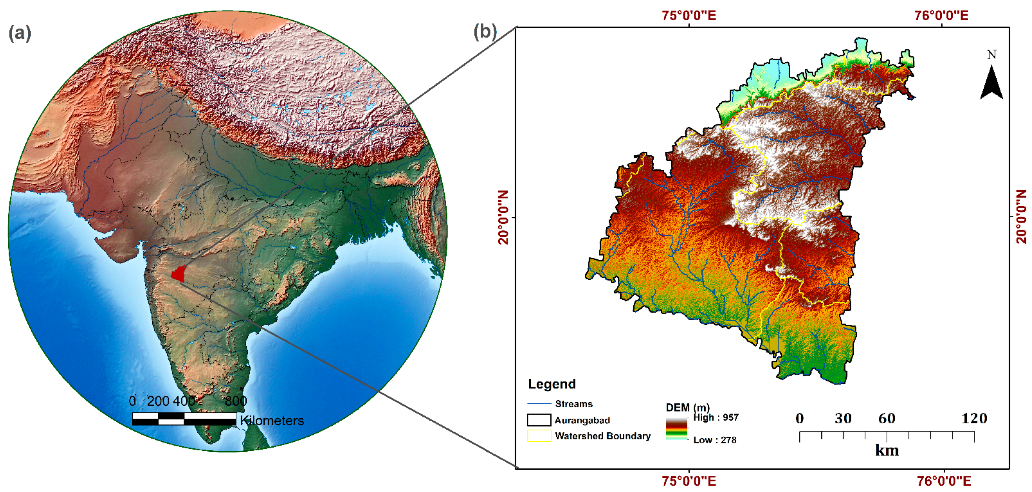
2. Study Area
3. Database and Methodology
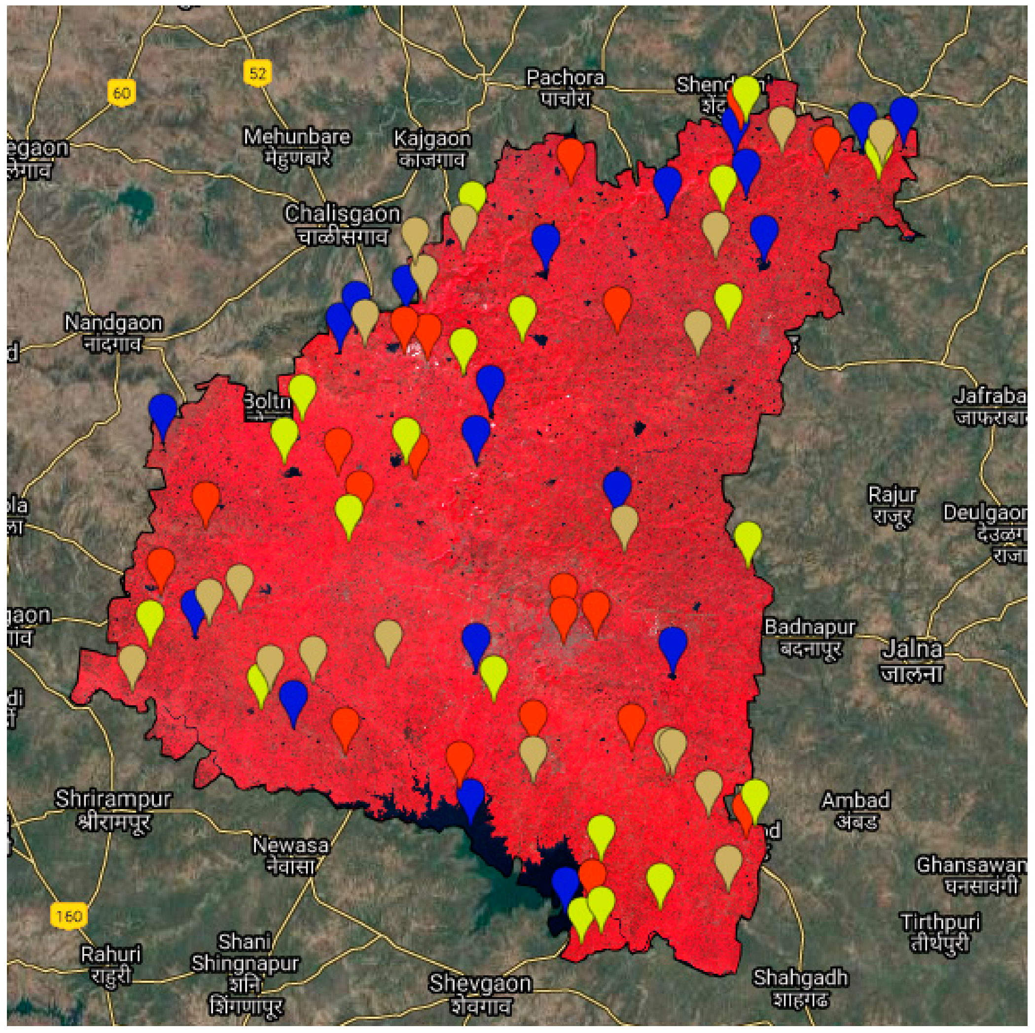
3.1. Satellite Datasets
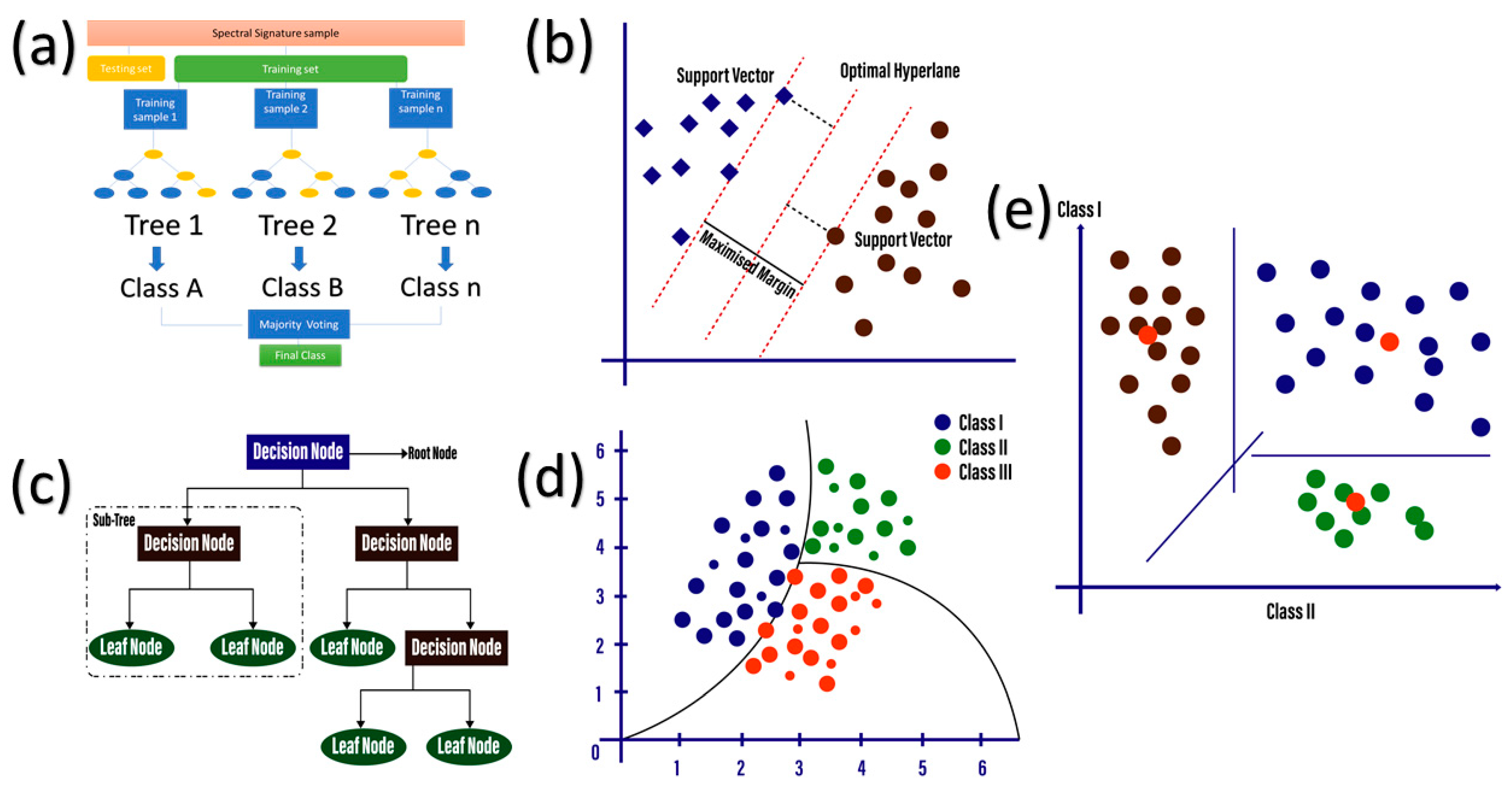
3.1.1. Random Forest Algorithm
3.1.2. Support Vector Machine
3.1.3. Classification and Regression Tree
3.1.4. Naïve Bayes (NB)
- P(c|x) is the posterior probability.
- P(c) is the prior probability of class.
- P(x|c) is the probability of predictor of a given class.
- P(x) is the prior probability of predictor.
3.1.5. Minimum Distance
3.2. Meteorological Parameters and Soil Moisture
3.2.1. Trend Analysis Using Mann–Kendall’s Test
3.2.2. Sen’s Slope Estimator for Magnitude of the Trend
3.3. Correlation and Multiple Linear Regression
- r = correlation coefficient
- xi = values of the x-variable in a sample
- = mean of the values of the x-variable
- yi = values of the y-variable in a sample
- = mean of the values of the y-variable Result
3.4. Limitations of the Study
4. Results
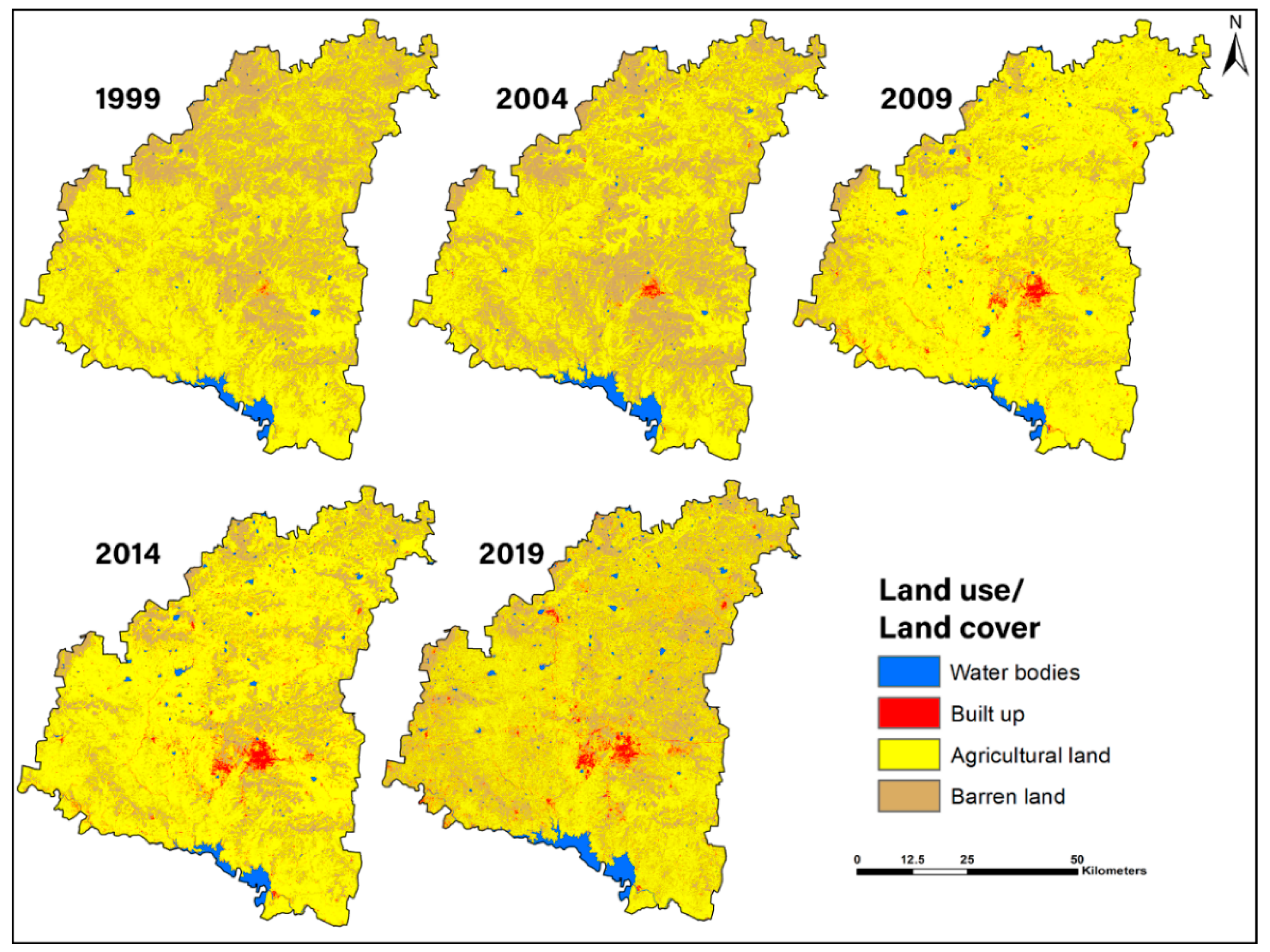
4.1. Temporal Analysis of Land Use/Land Cover
4.2. Temporal Analysis of Meteorological Parameters (1999–2019)
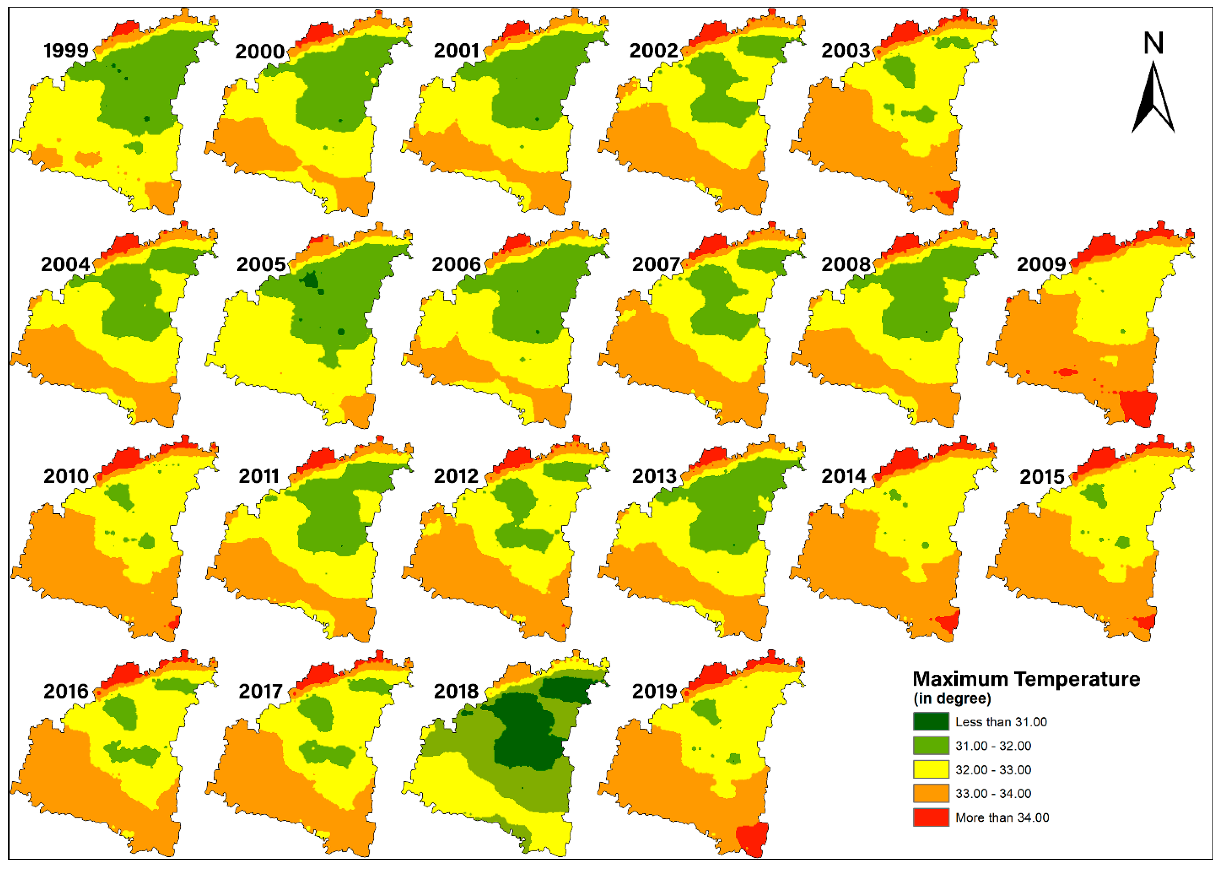
4.2.1. Maximum Temperature
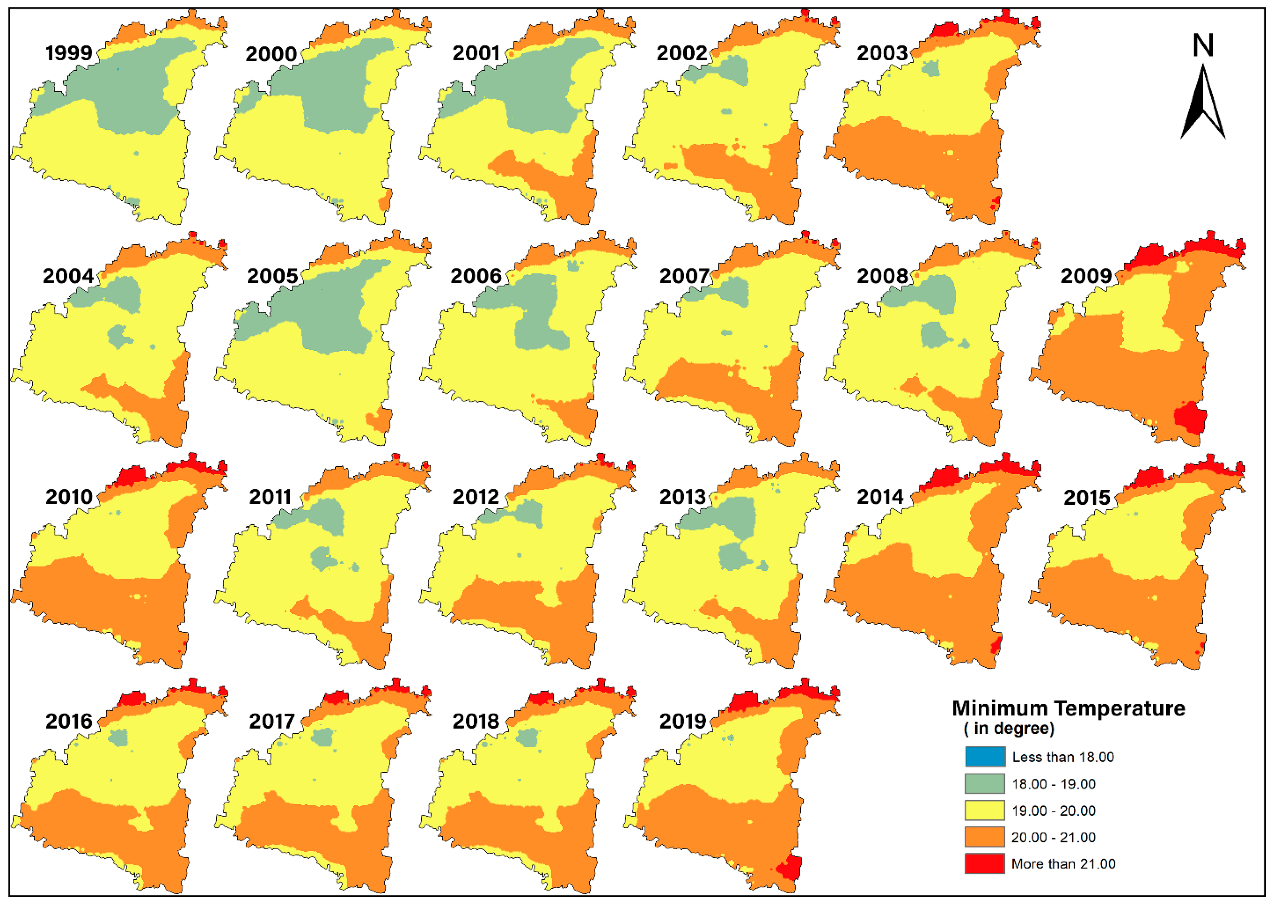
4.2.2. Minimum Temperature
4.2.3. Precipitation
4.2.4. Soil Moisture
4.2.5. Wind Speed
4.3. Correlation between LULC Change and Meteorological Parameters
4.4. Influence of Land Use/Land Cover Change on Meteorological Variables
5. Discussion
6. Conclusions
Author Contributions
Funding
Institutional Review Board Statement
Informed Consent Statement
Data Availability Statement
Acknowledgments
Conflicts of Interest
Appendix A
References
- Hua, A.K. Land Use Land Cover Changes in Detection of Water Quality: A Study Based on Remote Sensing and Multivariate Statistics. J. Environ. Public Health 2017, 2017, 7515130. [Google Scholar] [CrossRef] [Green Version]
- Chamling, M.; Bera, B. Spatio-Temporal Patterns of Land Use/Land Cover Change in the Bhutan–Bengal Foothill Region Between 1987 and 2019: Study Towards Geospatial Applications and Policy Making. Earth Syst. Environ. 2020, 4, 1–14. [Google Scholar] [CrossRef]
- Yesuph, A.Y.; Dagnew, A.B. Land Use/Cover Spatiotemporal Dynamics, Driving Forces and Implications at the Beshillo Catchment of the Blue Nile Basin, North Eastern Highlands of Ethiopia. Environ. Syst. Res. 2019, 8, 21. [Google Scholar] [CrossRef] [Green Version]
- Watson, R.T.; Noble, I.R.; Bolin, B.; Ravindranath, N.H.; Verardo, D.J.; Dokken, D.J. Land Use, Land-Use Change and Forestry: A Special Report of the Intergovernmental Panel on Climate Change; Cambridge University Press: Cambridge, UK, 2000. [Google Scholar]
- Romanowicz, R.J. The Impacts of Changes in Climate and Land Use on Hydrological Processes. Acta Geophys. 2017, 65, 785–787. [Google Scholar] [CrossRef] [Green Version]
- Agarwal, C.; Green, G.M.; Grove, J.M.; Evans, T.P.; Schweik, C.M. A Review and Assessment of Land-Use Change Models: Dynamics of Space, Time, and Human Choice; Gen. Tech. Rep. NE-297; U.S. Department of Agriculture, Forest Service, Northeastern Research Station: Newton Square, PA, USA, 2002; Volume 297, 61p. [CrossRef] [Green Version]
- Li, X.-H.; Liu, J.-L.; Gibson, V.; Zhu, Y.-G. Urban Sustainability and Human Health in China, East Asia and Southeast Asia. Curr. Opin. Environ. Sustain. 2012, 4, 436–442. [Google Scholar] [CrossRef]
- Chen, J.; Sun, B.-M.; Chen, D.; Wu, X.; Guo, L.-Z.; Wang, G. Land Use Changes and Their Effects on the Value of Ecosystem Services in the Small Sanjiang Plain in China. Sci. World J. 2014, 2014, e752846. [Google Scholar] [CrossRef] [Green Version]
- Pande, C.B.; Moharir, K.N.; Kumar Singh, S.; Varade, A.M.; Elbeltagi, A.; Khadri, S.F.R.; Choudhari, P. Estimation of Crop and Forest Biomass Resources in a Semi-Arid Region Using Satellite Data and GIS. J. Saudi Soc. Agric. Sci. 2021, 20, 302–311. [Google Scholar] [CrossRef]
- Swain, D.; Roberts, G.J.; Dash, J.; Vinoj, V.; Lekshmi, K.; Tripathy, S. Impact of Rapid Urbanization on the Microclimate of Indian Cities: A Case Study for the City of Bhubaneswar. In Land Surface and Cryosphere Remote Sensing III; International Society for Optics and Photonics: Bellingham, WA, USA, 2016; Volume 9877, p. 98772X. [Google Scholar] [CrossRef]
- Chadchan, J.; Shankar, R. An Analysis of Urban Growth Trends in the Post-Economic Reforms Period in India. Int. J. Sustain. Built Environ. 2012, 1, 36–49. [Google Scholar] [CrossRef] [Green Version]
- Bai, X.; McPhearson, T.; Cleugh, H.; Nagendra, H.; Tong, X.; Zhu, T.; Zhu, Y.-G. Linking Urbanization and the Environment: Conceptual and Empirical Advances. Annu. Rev. Environ. Resour. 2017, 42, 215–240. [Google Scholar] [CrossRef] [Green Version]
- Patra, S.; Sahoo, S.; Mishra, P.; Mahapatra, S.C. Impacts of Urbanization on Land Use/Cover Changes and Its Probable Implications on Local Climate and Groundwater Level. J. Urban Manag. 2018, 7, 70–84. [Google Scholar] [CrossRef]
- Avtar, R.; Herath, S.; Saito, O.; Gera, W.; Singh, G.; Mishra, B.; Takeuchi, K. Application of remote sensing techniques toward the role of traditional water bodies with respect to vegetation conditions. Environ. Dev. Sustain. 2014, 16, 995–1011. [Google Scholar] [CrossRef]
- Prasad, G.; Ramesh, M.V. Spatio-Temporal Analysis of Land Use/Land Cover Changes in an Ecologically Fragile Area—Alappuzha District, Southern Kerala, India. Nat. Resour. Res. 2019, 28, 31–42. [Google Scholar] [CrossRef]
- Hsieh, C.-M. Sustainable Planning and Design: Urban Climate Solutions for Healthy, Livable Urban and Rural Areas. J. Urban Manag. 2021, 10, 1–2. [Google Scholar] [CrossRef]
- Ramaiah, M.; Avtar, R. Urban Green Spaces and Their Need in Cities of Rapidly Urbanizing India: A Review. Urban Sci. 2019, 3, 94. [Google Scholar] [CrossRef] [Green Version]
- Ramaiah, M.; Avtar, R.; Rahman, M.M. Land Cover Influences on LST in Two Proposed Smart Cities of India: Comparative Analysis Using Spectral Indices. Land 2020, 9, 292. [Google Scholar] [CrossRef]
- GebreMedhin, A.; Biruh, W.; Govindu, V.; Demissie, B.; Mehari, A. Detection of Urban Land Use Land Cover Dynamics Using GIS and Remote Sensing: A Case Study of Axum Town, Northern Ethiopia. J. Indian Soc. Remote Sens. 2019, 47, 1209–1222. [Google Scholar] [CrossRef]
- Schellnhuber, H.J.; Hare, W.; Serdeczny, O.; Adams, S.; Coumou, D.; Frieler, K.; Martin, M.; Otto, I.M.; Perrette, M.; Robinson, A.; et al. Turn down the Heat: Why a 4 Deg C Warmer World Must Be Avoided; Sauvons le Climat-SLC: Paris, France, 2012; p. 110. [Google Scholar]
- Mahmood, R.; Jia, S.; Zhu, W. Analysis of Climate Variability, Trends, and Prediction in the Most Active Parts of the Lake Chad Basin, Africa. Sci. Rep. 2019, 9, 6317. [Google Scholar] [CrossRef] [Green Version]
- Hong, H.T.C.; Avtar, R.; Fujii, M. Monitoring changes in land use and distribution of mangroves in the southeastern part of the Mekong River Delta, Vietnam. Trop Ecol. 2019, 60, 552–565. [Google Scholar] [CrossRef]
- Gibril, M.B.A.; Bakar, S.A.; Yao, K.; Idrees, M.O.; Pradhan, B. Fusion of RADARSAT-2 and Multispectral Optical Remote Sensing Data for LULC Extraction in a Tropical Agricultural Area. Geocarto Int. 2017, 32, 735–748. [Google Scholar] [CrossRef]
- Wentz, E.A.; Nelson, D.; Rahman, A.; Stefanov, W.L.; Roy, S.S. Expert System Classification of Urban Land Use/Cover for Delhi, India. Int. J. Remote Sens. 2008, 29, 4405–4427. [Google Scholar] [CrossRef]
- As-syakur, A.R.; Adnyana, I.W.S.; Arthana, I.W.; Nuarsa, I.W. Enhanced Built-Up and Bareness Index (EBBI) for Mapping Built-Up and Bare Land in an Urban Area. Remote Sens. 2012, 4, 2957–2970. [Google Scholar] [CrossRef] [Green Version]
- Rwanga, S.S.; Ndambuki, J.M. Accuracy Assessment of Land Use/Land Cover Classification Using Remote Sensing and GIS. Int. J. Geosci. 2017, 8, 611. [Google Scholar] [CrossRef] [Green Version]
- Sahana, M.; Dutta, S.; Sajjad, H. Assessing Land Transformation and Its Relation with Land Surface Temperature in Mumbai City, India Using Geospatial Techniques. Int. J. Urban Sci. 2019, 23, 205–225. [Google Scholar] [CrossRef]
- Shaharum, N.S.N.; Shafri, H.Z.M.; Gambo, J.; Abidin, F.A.Z. Mapping of Krau Wildlife Reserve (KWR) Protected Area Using Landsat 8 and Supervised Classification Algorithms. Remote Sens. Appl. Soc. Environ. 2018, 10, 24–35. [Google Scholar] [CrossRef]
- Bazan, G.; Castrorao Barba, A.; Rotolo, A.; Marino, P. Geobotanical Approach to Detect Land-Use Change of a Mediterranean Landscape: A Case Study in Central-Western Sicily. GeoJournal 2019, 84, 795–811. [Google Scholar] [CrossRef]
- Sekertekin, A.; Marangoz, A.M.; Akcin, H. Pixel-based classification analysis of land use land cover using sentinel-2 and landsat-8 data. Int. Arch. Photogramm. Remote Sens. Spat. Inf. Sci. 2017, XLII-4/W6, 91–93. [Google Scholar] [CrossRef] [Green Version]
- Allam, M.; Bakr, N.; Elbably, W. Multi-Temporal Assessment of Land Use/Land Cover Change in Arid Region Based on Landsat Satellite Imagery: Case Study in Fayoum Region, Egypt. Remote Sens. Appl. Soc. Environ. 2019, 14, 8–19. [Google Scholar] [CrossRef]
- Jamali, A. Land Use Land Cover Mapping Using Advanced Machine Learning Classifiers: A Case Study of Shiraz City, Iran. Earth Sci. Inform. 2020, 13, 1015–1030. [Google Scholar] [CrossRef]
- Chang, Y.; Hou, K.; Li, X.; Zhang, Y.; Chen, P. Review of Land Use and Land Cover Change Research Progress. IOP Conf. Ser. Earth Environ. Sci. 2018, 113, 012087. [Google Scholar] [CrossRef]
- Surabuddin Mondal, M.; Sharma, N.; Kappas, M.; Garg, P.K. Modeling of Spatio-Temporal Dynamics of Land Use and Land Cover in a Part of Brahmaputra River Basin Using Geoinformatic Techniques. Geocarto Int. 2013, 28, 632–656. [Google Scholar] [CrossRef]
- Veldkamp, A.; Lambin, E.F. Predicting Land-Use Change. Agric. Ecosyst. Environ. 2001, 85, 1–6. [Google Scholar] [CrossRef]
- Regasa, M.S.; Nones, M.; Adeba, D. A Review on Land Use and Land Cover Change in Ethiopian Basins. Land 2021, 10, 585. [Google Scholar] [CrossRef]
- Singh, S.K.; Srivastava, P.K.; Gupta, M.; Thakur, J.K.; Mukherjee, S. Appraisal of Land Use/Land Cover of Mangrove Forest Ecosystem Using Support Vector Machine. Environ. Earth Sci. 2014, 71, 2245–2255. [Google Scholar] [CrossRef]
- Traoré, F.; Bonkoungou, J.; Compaoré, J.; Kouadio, L.; Wellens, J.; Hallot, E.; Tychon, B. Using Multi-Temporal Landsat Images and Support Vector Machine to Assess the Changes in Agricultural Irrigated Areas in the Mogtedo Region, Burkina Faso. Remote Sens. 2019, 11, 1442. [Google Scholar] [CrossRef] [Green Version]
- Wang, L.; Jia, Y.; Yao, Y.; Xu, D. Accuracy Assessment of Land Use Classification Using Support Vector Machine and Neural Network for Coal Mining Area of Hegang City, China. Nat. Environ. Pollut. Technol. 2019, 18, 335–341. [Google Scholar]
- Nooni, I.K.; Duker, A.A.; Van Duren, I.; Addae-Wireko, L.; Osei Jnr, E.M. Support Vector Machine to Map Oil Palm in a Heterogeneous Environment. Int. J. Remote Sens. 2014, 35, 4778–4794. [Google Scholar] [CrossRef]
- Hearst, M.A.; Dumais, S.T.; Osuna, E.; Platt, J.; Scholkopf, B. Support Vector Machines. IEEE Intell. Syst. Appl. 1998, 13, 18–28. [Google Scholar] [CrossRef] [Green Version]
- Evgeniou, T.; Pontil, M. Support Vector Machines: Theory and Applications. In Machine Learning and Its Applications: Advanced Lectures; Paliouras, G., Karkaletsis, V., Spyropoulos, C.D., Eds.; Springer: Berlin/Heidelberg, Germany, 2001; pp. 249–257. [Google Scholar] [CrossRef] [Green Version]
- Mo, Y.; Zhong, R.; Sun, H.; Wu, Q.; Du, L.; Geng, Y.; Cao, S. Integrated Airborne LiDAR Data and Imagery for Suburban Land Cover Classification Using Machine Learning Methods. Sensors 2019, 19, 1996. [Google Scholar] [CrossRef] [Green Version]
- Adam, E.; Mutanga, O.; Odindi, J.; Abdel-Rahman, E.M. Land-Use/Cover Classification in a Heterogeneous Coastal Landscape Using RapidEye Imagery: Evaluating the Performance of Random Forest and Support Vector Machines Classifiers. Int. J. Remote Sens. 2014, 35, 3440–3458. [Google Scholar] [CrossRef]
- Oliphant, A.J.; Thenkabail, P.S.; Teluguntla, P.; Xiong, J.; Gumma, M.K.; Congalton, R.G.; Yadav, K. Mapping Cropland Extent of Southeast and Northeast Asia Using Multi-Year Time-Series Landsat 30-m Data Using a Random Forest Classifier on the Google Earth Engine Cloud. Int. J. Appl. Earth Obs. Geoinf. 2019, 81, 110–124. [Google Scholar] [CrossRef]
- Yang, C.; Wu, G.; Ding, K.; Shi, T.; Li, Q.; Wang, J. Improving Land Use/Land Cover Classification by Integrating Pixel Unmixing and Decision Tree Methods. Remote Sens. 2017, 9, 1222. [Google Scholar] [CrossRef] [Green Version]
- Hu, Y.; Hu, Y. Land Cover Changes and Their Driving Mechanisms in Central Asia from 2001 to 2017 Supported by Google Earth Engine. Remote Sens. 2019, 11, 554. [Google Scholar] [CrossRef] [Green Version]
- Midekisa, A.; Holl, F.; Savory, D.J.; Andrade-Pacheco, R.; Gething, P.W.; Bennett, A.; Sturrock, H.J.W. Mapping Land Cover Change over Continental Africa Using Landsat and Google Earth Engine Cloud Computing. PLoS ONE 2017, 12, e0184926. [Google Scholar] [CrossRef]
- Alexander, L.V.; Zhang, X.; Peterson, T.C.; Caesar, J.; Gleason, B.; Tank, A.M.G.K.; Haylock, M.; Collins, D.; Trewin, B.; Rahimzadeh, F.; et al. Global Observed Changes in Daily Climate Extremes of Temperature and Precipitation. J. Geophys. Res. Atmos. 2006, 111, D05109. [Google Scholar] [CrossRef] [Green Version]
- Pielke, R.A.; Adegoke, J.; BeltraáN-Przekurat, A.; Hiemstra, C.A.; Lin, J.; Nair, U.S.; Niyogi, D.; Nobis, T.E. An Overview of Regional Land-Use and Land-Cover Impacts on Rainfall. Tellus B Chem. Phys. Meteorol. 2007, 59, 587–601. [Google Scholar] [CrossRef]
- Gogoi, P.P.; Vinoj, V.; Swain, D.; Roberts, G.; Dash, J.; Tripathy, S. Land Use and Land Cover Change Effect on Surface Temperature over Eastern India. Sci. Rep. 2019, 9, 8859. [Google Scholar] [CrossRef] [Green Version]
- Masroor, M.; Rehman, S.; Sajjad, H.; Rahaman, M.H.; Sahana, M.; Ahmed, R.; Singh, R. Assessing the Impact of Drought Conditions on Groundwater Potential in Godavari Middle Sub-Basin, India Using Analytical Hierarchy Process and Random Forest Machine Learning Algorithm. Groundw. Sustain. Dev. 2021, 13, 100554. [Google Scholar] [CrossRef]
- Aher, K.R.; Deshpande, S.M. Assessment of Water Quality of the Maniyad Reservoir of Parala Village, District Aurangabad: Suitability for Multipurpose Usage. Int. J. Recent Trends Sci. Technol. 2011, 1, 91–95. [Google Scholar]
- Ragade, G.S.; Dhumal, R.; Gawali, B.W. Analysis and Modelling of Drinking Water Utilities by Using GIS: In Aurangabad City, Maharashtra, India. CSIT 2018, 6, 77–81. [Google Scholar] [CrossRef]
- Teluguntla, P.; Thenkabail, P.S.; Oliphant, A.; Xiong, J.; Gumma, M.K.; Congalton, R.G.; Yadav, K.; Huete, A. A 30-m Landsat-Derived Cropland Extent Product of Australia and China Using Random Forest Machine Learning Algorithm on Google Earth Engine Cloud Computing Platform. ISPRS J. Photogramm. Remote Sens. 2018, 144, 325–340. [Google Scholar] [CrossRef]
- Masroor, M.; Rehman, S.; Avtar, R.; Sahana, M.; Ahmed, R.; Sajjad, H. Exploring Climate Variability and Its Impact on Drought Occurrence: Evidence from Godavari Middle Sub-Basin, India. Weather Clim. Extrem. 2020, 30, 100277. [Google Scholar] [CrossRef]
- Rodriguez-Galiano, V.F.; Ghimire, B.; Rogan, J.; Chica-Olmo, M.; Rigol-Sanchez, J.P. An Assessment of the Effectiveness of a Random Forest Classifier for Land-Cover Classification. ISPRS J. Photogramm. Remote Sens. 2012, 67, 93–104. [Google Scholar] [CrossRef]
- Oliphant, A.J.; Thenkabail, P.S.; Teluguntla, P.; Xiong, J.; Congalton, R.G.; Yadav, K.; Massey, R.; Gumma, M.K.; Smith, C. NASA Making Earth System Data Records for Use in Research Environments (MEaSUREs) Global Food Security-Support Analysis Data (GFSAD) Cropland Extent 2015 Southeast Asia 30 m V001. Available online: https://lpdaac.usgs.gov/dataset_discovery/measures/measures_products_table/gfsad30seace_v001 (accessed on 5 August 2021).
- Rahmati, O.; Choubin, B.; Fathabadi, A.; Coulon, F.; Soltani, E.; Shahabi, H.; Mollaefar, E.; Tiefenbacher, J.; Cipullo, S.; Ahmad, B.B.; et al. Predicting Uncertainty of Machine Learning Models for Modelling Nitrate Pollution of Groundwater Using Quantile Regression and UNEEC Methods. Sci. Total Environ. 2019, 688, 855–866. [Google Scholar] [CrossRef] [PubMed]
- Vapnik, V.N.; Chervonenkis, A.Y. On the Uniform Convergence of Relative Frequencies of Events to Their Probabilities. Theory Probab. Appl. 1971, 16, 264–280. [Google Scholar] [CrossRef]
- Osuna, E.; Freund, R.; Girosi, F. Support Vector Machines: Training and Applications. Ph.D. Thesis, Massachusetts Institute of Technology, Cambridge, MA, USA, 1997. [Google Scholar]
- Pal, M. Factors Influencing the Accuracy of Remote Sensing Classifications: A Comparative Study. Available online: http://eprints.nottingham.ac.uk/10314/ (accessed on 12 November 2021).
- Shetty, S. Analysis of Machine Learning Classifiers for LULC Classification on Google Earth Engine. Available online: http://essay.utwente.nl/83543/ (accessed on 12 November 2021).
- John, G.H.; Langley, P. Estimating Continuous Distributions in Bayesian Classifiers. In Proceedings of the Eleventh Conference on Uncertainty in Artificial Intelligence (UAI’95), Montreal, QC, Canada, 18–20 August 1995; Morgan Kaufmann Publishers Inc.: San Francisco, CA, USA, 1995; pp. 338–345. [Google Scholar]
- Zhang, H. Exploring Conditions for the Optimality of Naïve Bayes. Int. J. Pattern Recogn. Artif. Intell. 2005, 19, 183–198. [Google Scholar] [CrossRef]
- Devi, M.R. Land Use and Land Cover Classification Using RGB&L Based Supervised Classification Algorithm. Eng. Technol. 2011, 2, 14. [Google Scholar]
- Abatzoglou, J.T.; Dobrowski, S.Z.; Parks, S.A.; Hegewisch, K.C. TerraClimate, a High-Resolution Global Dataset of Monthly Climate and Climatic Water Balance from 1958–2015. Sci. Data 2018, 5, 1–12. [Google Scholar] [CrossRef] [Green Version]
- Pearson, K.; Galton, F. VII. Note on Regression and Inheritance in the Case of Two Parents. Proc. R. Soc. Lond. 1895, 58, 240–242. [Google Scholar] [CrossRef]
- Mudelsee, M. (Ed.) Introduction. In Climate Time Series Analysis: Classical Statistical and Bootstrap Methods; Atmospheric and Oceanographic Sciences Library; Springer International Publishing: Cham, Switzerland, 2014; pp. 3–30. [Google Scholar] [CrossRef]
- Tundisi, J.G.; Matsumura-Tundisi, T.; Arantes Junior, J.D.; Tundisi, J.E.M.; Manzini, N.F.; Ducrot, R. The Response of Carlos Botelho (Lobo, Broa) Reservoir to the Passage of Cold Fronts as Reflected by Physical, Chemical, and Biological Variables. Braz. J. Biol. 2004, 64, 177–186. [Google Scholar] [CrossRef] [Green Version]
- Nagne, A.D.; Vibhute, A.D.; Dhumal, R.K.; Kale, K.V.; Mehrotra, S.C. Urban LULC Change Detection and Mapping Spatial Variations of Aurangabad City Using IRS LISS-III Temporal Datasets and Supervised Classification Approach. In Data Analytics and Learning; Nagabhushan, P., Guru, D.S., Shekar, B.H., Kumar, Y.H.S., Eds.; Lecture Notes in Networks and Systems; Springer: Singapore, 2019; pp. 369–386. [Google Scholar] [CrossRef]
- Ghosh, S.; Deshmukh, M. Naïve Geolocation of Urban Heat Islands in Aurangabad City (Maharashtra State) Using Remote Sensing and Ancillary Data. In Proceedings of the 2020 International Conference on Smart Innovations in Design, Environment, Management, Planning and Computing (ICSIDEMPC), Aurangabad, India, 30–31 October 2020; pp. 341–346. [Google Scholar] [CrossRef]
- Bataille, C.G.F. Physical and Policy Pathways to Net-Zero Emissions Industry. WIREs Clim. Chang. 2020, 11, e633. [Google Scholar] [CrossRef]


| Classifier | Model Accuracy | Field Data Accuracy | Overall Accuracy |
|---|---|---|---|
| CART | 0.74 | 0.78 | 0.76 |
| Random Forest | 0.84 | 0.89 | 0.86 |
| SVM | 0.84 | 0.86 | 0.85 |
| Continuous Naive | 0.85 | 0.81 | 0.83 |
| Minimum Distance | 0.81 | 0.84 | 0.83 |
| Class | 1999 | 2004 | 2009 | 2014 | 2019 | |||||
|---|---|---|---|---|---|---|---|---|---|---|
| Area (km2) | Area (%) | Area (km2) | Area (%) | Area (km2) | Area (%) | Area (km2) | Area (%) | Area (km2) | Area (%) | |
| Water bodies | 180.8 | 1.68 | 243.5 | 2.26 | 232.6 | 2.16 | 236.7 | 2.20 | 350.9 | 3.26 |
| Built-up | 65.4 | 0.61 | 79.2 | 0.74 | 225.8 | 2.10 | 470.4 | 4.37 | 525.4 | 4.89 |
| Agricultural land | 6430.0 | 59.78 | 6123.4 | 56.93 | 8745.5 | 81.31 | 7807.4 | 72.59 | 5697.1 | 52.97 |
| Barren Land | 4079.3 | 37.93 | 4309.5 | 40.07 | 1551.5 | 14.43 | 2241 | 20.84 | 4182.1 | 38.88 |
| Total | 10,755.5 | 100 | 10,755.5 | 100 | 10,755.5 | 100 | 10,755.5 | 100 | 10,755.5 | 100 |
| Months | Minimum | Maximum | Mean | SD | ZMK | Prewhitened Sen’s Slope | Sen’s Slope | p-Value |
|---|---|---|---|---|---|---|---|---|
| January | 27.8 | 34.0 | 29.1 | 1.3 | −1.655 * | −0.059 | −0.036 | 0.0980 |
| February | 30.8 | 34.0 | 32.5 | 0.9 | −0.746 | −0.028 | −0.020 | 0.4555 |
| March | 34.3 | 38.0 | 36.1 | 0.9 | −0.162 | −0.011 | −0.032 | 0.8711 |
| April | 37.2 | 40.4 | 38.9 | 0.7 | −0.552 | −0.012 | −0.010 | 0.5813 |
| May | 38.3 | 41.6 | 40.1 | 0.8 | 3.926 *** | 0.107 | 0.105 | 0.0001 |
| June | 33.1 | 37.1 | 34.8 | 1.1 | 2.174 ** | 0.129 | 0.110 | 0.0297 |
| July | 27.6 | 31.7 | 30.0 | 0.8 | 0.811 | 0.019 | 0.028 | 0.4173 |
| August | 28.2 | 31.1 | 29.6 | 0.7 | 1.784 * | 0.042 | 0.052 | 0.0744 |
| September | 28.7 | 31.2 | 30.0 | 0.6 | 0.032 | 0.005 | 0.015 | 0.9741 |
| October | 30.3 | 32.9 | 31.6 | 0.7 | 0.811 | 0.024 | 0.024 | 0.4173 |
| November | 28.9 | 32.1 | 30.6 | 0.8 | −0.487 | −0.018 | −0.006 | 0.6265 |
| December | 27.4 | 30.5 | 29.3 | 0.8 | −0.292 | −0.017 | −0.009 | 0.7703 |
| Months | Minimum | Maximum | Mean | SD | ZMK | Prewhitened Sen’s Slope | Sen’s Slope | p-Value |
|---|---|---|---|---|---|---|---|---|
| January | 12.2 | 18.3 | 13.5 | 1.3 | −0.8111 | −0.0211 | −0.0106 | 0.4173 |
| February | 14.7 | 17.8 | 16.5 | 0.9 | −0.0973 | −0.0048 | −0.0042 | 0.9225 |
| March | 17.9 | 21.6 | 19.7 | 1.0 | 0.5516 | 0.0308 | 0.0215 | 0.5813 |
| April | 22.4 | 25.5 | 24.1 | 0.7 | −0.6164 | −0.0154 | −0.0157 | 0.5376 |
| May | 23.9 | 27.0 | 25.5 | 0.7 | 4.0555 *** | 0.1106 | 0.0994 | 0.0001 |
| June | 22.3 | 25.9 | 23.6 | 1.1 | 2.5631 ** | 0.1282 | 0.1021 | 0.0104 |
| July | 21.5 | 24.0 | 22.5 | 0.6 | 0.6164 | 0.0185 | 0.0226 | 0.5376 |
| August | 20.9 | 23.2 | 21.8 | 0.6 | 1.9142 * | 0.0403 | 0.0545 | 0.0556 |
| September | 20.1 | 22.4 | 21.1 | 0.5 | 0.8760 | 0.0214 | 0.0255 | 0.3810 |
| October | 18.4 | 21.0 | 19.6 | 0.7 | 0.5516 | 0.0212 | 0.0314 | 0.5813 |
| November | 14.5 | 17.7 | 16.1 | 0.8 | 1.0707 | 0.0301 | 0.0413 | 0.2843 |
| December | 11.7 | 14.6 | 13.3 | 0.9 | 0.0324 | 0.0006 | 0.0369 | 0.9741 |
| Months | Minimum | Maximum | Mean | SD | ZMK | Prewhitened Sen’s Slope | Sen’s Slope | p-Value |
|---|---|---|---|---|---|---|---|---|
| January | 0.0 | 12.1 | 1.7 | 2.9 | −2.6005 | −1.2801 | 0 | 7.9482 |
| February | 0.0 | 3.6 | 0.8 | 1.1 | 6.5014 | 1.1968 | 0 | 9.4816 |
| March | 0.0 | 26.7 | 5.8 | 7.7 | −2.9199 | −4.4345 | 3.5388 | 7.7028 |
| April | 0.0 | 16.9 | 4.5 | 4.7 | 1.2004 | 2.0696 | 1.2283 | 2.2996 |
| May | 0.0 | 71.4 | 18.8 | 19.0 | −1.1355 | −7.4434 | −5.3695 | 2.5614 |
| June | 18.7 | 250.1 | 142.3 | 53.4 | −1.8493 | −4.0923 | −1.4622 | 6.4411 |
| July | 31.2 | 263.5 | 165.3 | 64.1 | 8.7599 | 2.177 | 3.1491 | 3.8103 |
| August | 54.3 | 313.6 | 152.0 | 56.5 | −8.7599 | −1.2975 | −1.1899 | 3.8103 |
| September | 46.8 | 262.4 | 153.4 | 58.7 | 1.6546 | 5.8286 | 4.4866 | 9.7993 |
| October | 1.2 | 242.1 | 56.7 | 50.7 | 1.1355 | 1.6098 | 8.9211 | 2.5614 |
| November | 0.0 | 185.8 | 21.8 | 41.4 | 8.111 | 3.4544 | 3.0979 | 4.173 |
| December | 0.0 | 21.2 | 3.4 | 5.7 | 8.8378 | 6.9348 | 0 | 3.7681 |
| Months | Minimum | Maximum | Mean | SD | ZMK | Prewhitened Sen’s Slope | Sen’s Slope | p-Value |
|---|---|---|---|---|---|---|---|---|
| January | 6.3 | 36.4 | 20.2 | 6.5 | 0.1622 | 0.0762 | 0.0350 | 0.8711 |
| February | 6.0 | 26.9 | 16.8 | 4.6 | 0.0324 | 0.0169 | 0.0224 | 0.9741 |
| March | 5.7 | 21.6 | 14.4 | 3.6 | 0.0324 | 0.0298 | 0.0141 | 0.9741 |
| April | 5.4 | 18.0 | 12.7 | 2.9 | 0.1622 | 0.0311 | 0.0093 | 0.8711 |
| May | 5.2 | 15.5 | 11.3 | 2.4 | 0.1622 | 0.0253 | 0.0063 | 0.8711 |
| June | 8.2 | 91.9 | 19.8 | 19.8 | 0.2271 | 0.0337 | 0.0430 | 0.8203 |
| July | 8.9 | 115.7 | 58.8 | 39.5 | 0.4867 | 1.0539 | 1.3363 | 0.6265 |
| August | 9.0 | 121.3 | 70.6 | 37.8 | 0.2271 | 0.0501 | 0.9217 | 0.8203 |
| September | 8.3 | 121.4 | 83.8 | 34.8 | 0.4867 | 0.9886 | 1.1060 | 0.6265 |
| October | 7.7 | 121.4 | 55.3 | 28.0 | 1.2004 | 1.8144 | 1.4012 | 0.2300 |
| November | 7.2 | 115.3 | 39.2 | 25.0 | 0.9409 | 0.5473 | 0.5752 | 0.3468 |
| December | 6.7 | 60.3 | 26.4 | 11.5 | 0.8111 | 0.3567 | 0.3414 | 0.4173 |
| Months | Minimum | Maximum | Mean | SD | ZMK | Prewhitened Sen’s Slope | Sen’s Slope | p-Value |
|---|---|---|---|---|---|---|---|---|
| January | 8.9 | 18.3 | 16.1 | 1.9 | −2.5631 ** | −0.1699 | −0.1330 | 0.0104 |
| February | 6.3 | 18.2 | 15.5 | 2.5 | −0.6813 | −0.0433 | −0.0424 | 0.4957 |
| March | 6.9 | 20.2 | 16.1 | 2.8 | −3.1471 *** | −0.3690 | −0.1830 | 0.0016 |
| April | 14.4 | 25.8 | 19.6 | 3.1 | −2.0440 ** | −0.2143 | −0.2609 | 0.0410 |
| May | 25.2 | 38.4 | 32.2 | 3.5 | −2.3684 ** | −0.2823 | −0.2841 | 0.0179 |
| June | 22.0 | 39.8 | 32.5 | 4.8 | −2.5631 ** | −0.5167 | −0.4070 | 0.0104 |
| July | 26.4 | 46.5 | 35.8 | 6.0 | 0.3569 | 0.1187 | 0.0732 | 0.7212 |
| August | 18.3 | 41.2 | 28.4 | 5.8 | −1.1355 | −0.2193 | −0.2193 | 0.2561 |
| September | 13.0 | 28.6 | 20.7 | 4.2 | 0.0973 | 0.0579 | −0.0714 | 0.9225 |
| October | 5.9 | 13.3 | 10.1 | 1.9 | −3.0173 *** | −0.2464 | −0.1341 | 0.0026 |
| November | 6.6 | 15.1 | 11.9 | 2.2 | −0.4218 | −0.0607 | −0.0838 | 0.6732 |
| December | 10.0 | 15.7 | 13.3 | 1.4 | −1.2004 | −0.0903 | −0.0919 | 0.2300 |
| Variables | Waterbodies | Built-Up | Agricultural Land | Barren Land | Soil Moisture | Minimum Temperature | Maximum Temperature | Precipitation | Wind Speed |
|---|---|---|---|---|---|---|---|---|---|
| Waterbodies | 1 | ||||||||
| Built-up | 0.732 | 1 | |||||||
| Agricultural land | −0.402 | 0.034 | 1 | ||||||
| Barren Land | 0.228 | −0.237 | −0.979 ** | 1 | |||||
| Soil Moisture | −0.187 | 0.221 | 0.972 ** | −0.993 ** | 1 | ||||
| Minimum temperature | 0.142 | 0.417 | 0.806 | −0.877 | 0.877 | 1 | |||
| Maximum temperature | −0.549 | −0.173 | 0.881 * | −0.819 | 0.781 | 0.73 | 1 | ||
| Precipitation | −0.468 | −0.502 | 0.735 | −0.622 | 0.672 | 0.501 | 0.687 | 1 | |
| Wind Speed | −0.947* | −0.765 | 0.192 | −0.016 | −0.042 | −0.257 | 0.473 | 0.296 | 1 |
| Climatic Factors/LULC | Agricultural Land | t | Barren Land | t | Built-Up | t | Water Bodies | t |
|---|---|---|---|---|---|---|---|---|
| Precipitation | 0.735 | 1.878 | −1.1 * | −10.461 | −1.303 * | −8.668 | 0.737 | 4.916 |
| Maximum Temperature | 0.881 ** | 3.23 | −0.829 | −1.527 | 0.228 | 0.294 | −0.193 | −0.249 |
| Minimum Temperature | 0.806 | 2.358 | −1.068 | −2.758 | −0.256 | −0.462 | 0.573 | 1.037 |
| Soil Moisture | 0.972 *** | 7.208 | −1.073 * | −12.314 | −0.165 | −1.324 | 0.179 | 1.438 |
| Wind Speed | 0.192 | 0.338 | 0.232 | 0.733 | 0.050 | 0.110 | −1.037 | −2.296 |
Publisher’s Note: MDPI stays neutral with regard to jurisdictional claims in published maps and institutional affiliations. |
© 2022 by the authors. Licensee MDPI, Basel, Switzerland. This article is an open access article distributed under the terms and conditions of the Creative Commons Attribution (CC BY) license (https://creativecommons.org/licenses/by/4.0/).
Share and Cite
Masroor, M.; Avtar, R.; Sajjad, H.; Choudhari, P.; Kulimushi, L.C.; Khedher, K.M.; Komolafe, A.A.; Yunus, A.P.; Sahu, N. Assessing the Influence of Land Use/Land Cover Alteration on Climate Variability: An Analysis in the Aurangabad District of Maharashtra State, India. Sustainability 2022, 14, 642. https://doi.org/10.3390/su14020642
Masroor M, Avtar R, Sajjad H, Choudhari P, Kulimushi LC, Khedher KM, Komolafe AA, Yunus AP, Sahu N. Assessing the Influence of Land Use/Land Cover Alteration on Climate Variability: An Analysis in the Aurangabad District of Maharashtra State, India. Sustainability. 2022; 14(2):642. https://doi.org/10.3390/su14020642
Chicago/Turabian StyleMasroor, Md, Ram Avtar, Haroon Sajjad, Pandurang Choudhari, Luc Cimusa Kulimushi, Khaled Mohamed Khedher, Akinola Adesuji Komolafe, Ali P. Yunus, and Netrananda Sahu. 2022. "Assessing the Influence of Land Use/Land Cover Alteration on Climate Variability: An Analysis in the Aurangabad District of Maharashtra State, India" Sustainability 14, no. 2: 642. https://doi.org/10.3390/su14020642