Cyclic Behaviour of Uniform Sand in Drained and Undrained Conditions at Low Confining Stress in Small-Scale Landslide Model

Abstract

Earthquakes are one of the main landslide-triggering factors. Earthquakes induce cyclic shear stresses and strains in soil and raise pore water pressure, degrading soil strength towards slope failure. Slopes on which shallow landslides can form due to geological conditions are most susceptible to such failures, mainly because of low confining stress. Effective confining stress has a significant role on soil response during static and cyclic loading. Under low confining stress, soil exhibits dilatant behaviour and can degrade rapidly under cyclic loading. This paper presents the results of undrained and drained cyclic triaxial tests on uniform sandy soil material used for modelling small-scale shallow landslides under 1g conditions. Based on the scaling laws for a model in 1g conditions, the frequencies of straining amplitudes for strain-controlled cyclic triaxial tests were defined. Undrained and drained cyclic triaxial tests on the type of sand used in small-scale landslide models were performed. The sandy samples had been previously consolidated at low confining stress corresponding to the values present in the shallow landslides used as the prototype. The influences of loading frequency and low confining stress on sand behaviour were investigated, and simple models for pore pressure build-up and volumetric strain on sand behaviour were proposed. These simple models can be used to estimate increasing pore water pressure and volumetric strain due to cyclic loading at low confining stress for frequencies lower than 1 Hz. The proposed models show good correlation with the data obtained in the laboratory test.

1. Introduction

Earthquakes are considered to be one of the major landslide-triggering factors [1,2,3]. Earthquakes induce shear-wave propagation, causing cyclic shear stresses and strains that degrade the soil strength and generate pore-pressure build-up. This, in turn, leads to soil failure, and under some special site conditions, it can lead to soil liquefaction. Such behaviour is critical for slopes that are prone to shallow landslides. Shallow landslides are considered to have a depth of up to around five meters [4] and are greatly affected by earthquakes and rainfall (e.g., [5,6]). Significant research has been conducted on the activation of shallow landslides in volcanic soil, common for regions in Japan [7,8,9,10] and Italy [11,12,13,14]. Two approaches to landslide analysis have been established: (i) a pre-failure approach and (ii) a post-failure approach. 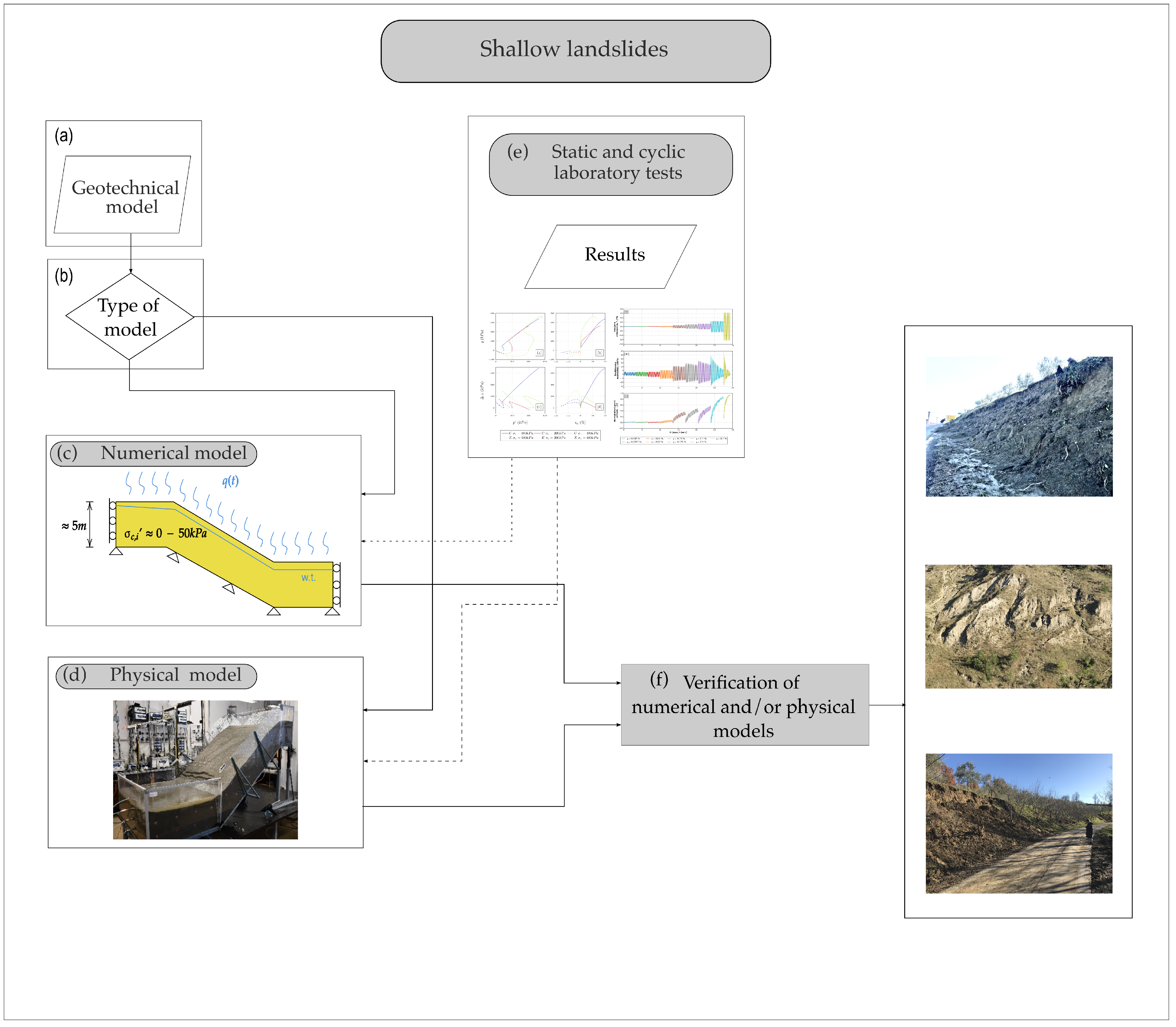In a pre-failure approach, slopes that have potential of failure and landslide activation are analysed and are often monitored as part of early warning systems (e.g., [15,16,17]). For a slope that has the potential to slide, an engineering geologist can determine a geological model as the basis of a geotechnical model (Figure 1a) from field exploration and laboratory testing. In a post-failure approach, the same procedure can be applied but with known slip-surface depth and mobilized strength parameters obtained through laboratory testing (e.g., [18,19,20,21]). It is not important which approach is used to analyse a slope; both can be used to create a numerical (Figure 1c) or physical model (Figure 1d) of the slope through a decision loop (Figure 1b). Physical modelling can be divided into two categories: (i) physical models at 1g (e.g., [22,23,24,25,26,27,28,29,30]) and (ii) physical models at ng (e.g., [31,32,33,34,35,36]). The first category is often simply used in laboratories where dimensions and other model elements (e.g., grain-size distribution, rain intensity, etc.) are scaled according to a decided scale factor, but the vertical acceleration is 1g. The second category requires sophisticated equipment or a geotechnical centrifuge to simulate larger values of gravitational acceleration: called ng conditions [37]. Models used in geotechnical centrifuges usually have significantly smaller dimensions than those used at 1g. Physical modelling of small-scale landslides under 1g conditions started at the end of 1980s, when the behaviour of flowslides and liquefaction were investigated [38]. Physical modelling under dynamic loading started in the mid 1950s [39], while simulations of seismically induced landslides were first developed in the early 2000s. Most of the known research concerns seismic behaviour and the response of slopes and slope material (e.g., [27,28,33,40,41]). Physical methods for assessing the stability of slopes during an earthquake were proposed by Jibson [42] and are still used today. A common feature of both numerical and physical models is the static and/or cyclic behaviour of materials (Figure 1e). It is necessary to determine static and/or cyclic behaviour of soil material used in models/simulations to accurately test landslide mechanisms. This is necessary for the analysis of, for example, rain infiltration, landslide run-off, erosion, degradation, and strength reduction due to cyclic loading. Results from both numerical and physical models have to be verified (Figure 1f) in order to calibrate the numerical model, refine boundary conditions of the physical model, and select appropriate material behaviour for laboratory tests.

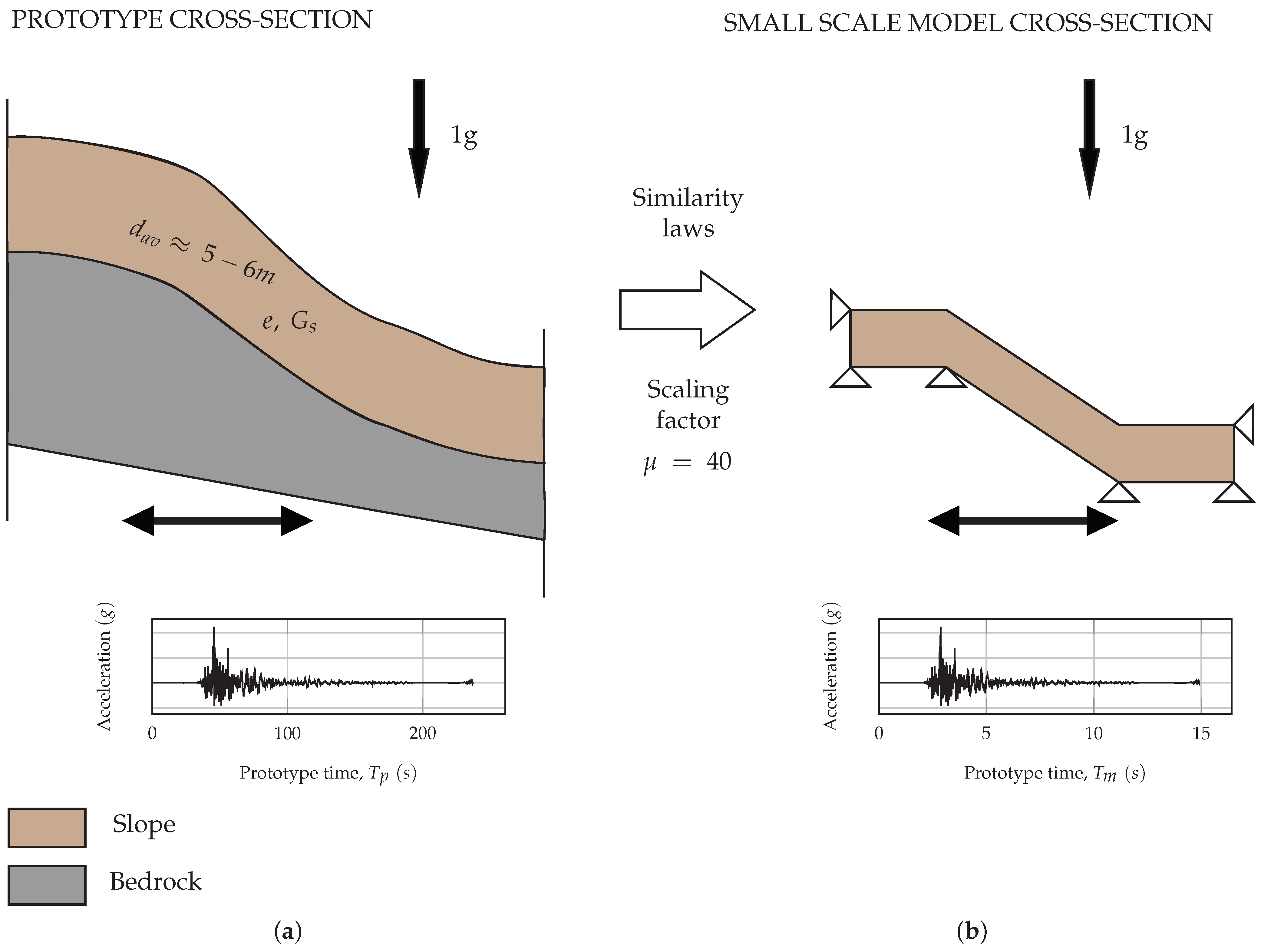
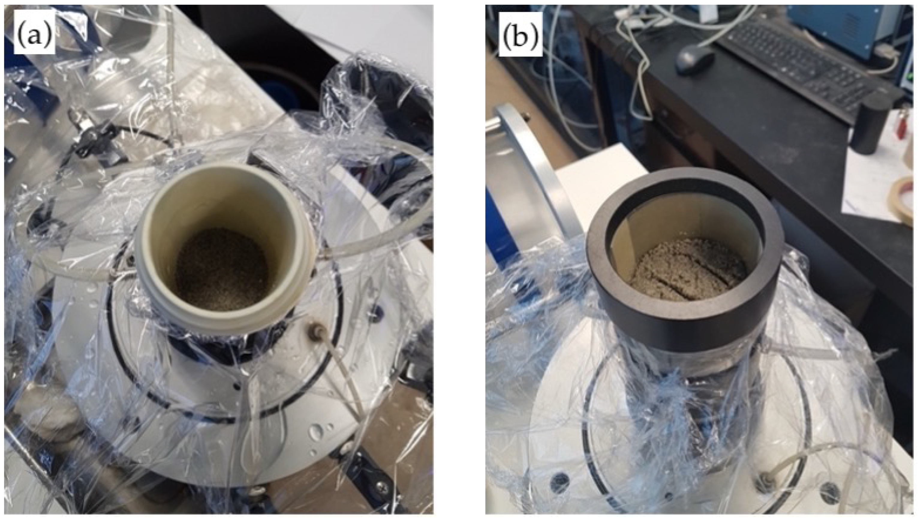
As part of ongoing research on landslide activation at 1g conditions, we subject slope material to dynamic loading to determine its behaviour [22]. A slope that has the potential to become a shallow landslide (Figure 2a) is scaled by a factor of 40 and dynamically loaded (Figure 2b), such as would occur during an earthquake. Dynamic loading conditions are applied with a seismic platform, as explained in detail later.

Frequencies of straining amplitudes for strain-controlled cyclic triaxial tests are defined based on similarity laws for 1g conditions [43] and small-scale landslide model dimensions (Figure 2). The corresponding frequencies with respect to similarity law are used for dynamic loading of slope material. Sandy specimens are tested at low confining stresses that correspond to a shallow landslide forming on a prototypical slope (Figure 2), ranging from 10 to 50 kPa. It is also assumed that the material used in the model is fully saturated, (as in post-rainfall conditions).

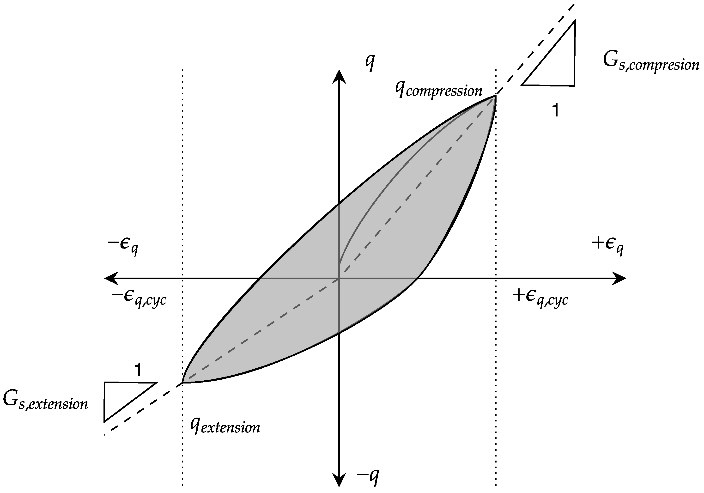
The behaviour of soil in shallow landslides is governed by low confining stress [44]. Low confining stress has a significant influence on soil strength, especially if the soil’s material strength is pressure-dependent. White [44] performed experiments in a triaxial cyclic device at low effective stresses (less than 50 kPa). All undrained cyclic tests were performed after isotropic consolidation until initial liquefaction had been reached. Such stress values correspond to a stress level in a slope at a depth less than 10 m from the soil surface. Higher confining stress values lead to a faster rise of pore pressure. The secant shear modulus, $G_s$, was found to decrease with an increasing number of cycles and with decreasing effective stress, ${\sigma }_{c,0}^{\prime }$ [44]. Test results of an equivalent viscous ratio show significant noise in the data, especially for lower cyclic load values, which in some experiments makes it difficult to reliably estimate damping ratio [44]. The results show that when the shear cyclic strain ${\gamma }_{cyc}$ is less than approximately ${10}^{(-4)}$%, the damping of soil does not significantly increase and remains relatively the same with the increasing number of cycles. This coincides with the literature [45,46,47,48], where the cyclic volumetric shear stress threshold ${\gamma }_{tv}$ is equal to ${10}^{(-4)}$% regardless of the effective stress, compaction, and sample structure. Once this threshold is exceeded, the damping of soil changes with the change in shear cyclic deformation and the number of cycles. Kumar et al. [3] found that samples tested at lower effective stresses (50 kPa) show a higher damping ratio compared to that of higher effective stresses (100 and 150 kPa), which was attributed to relatively higher stiffness due to sample constraints. Chakraborty and Salgado [49] conducted triaxial compression in drained conditions, along with in-plane compression experiments (plane-strain). The sand was tested at low effective stresses to determine the dependence of dilatation and friction angle related to relative compaction and applied effective stresses. The authors concluded that sand dilatation decreases with decreasing compaction and increasing applied effective stresses. Further, it was observed that for lower effective stresses (less than 50 kPa) had larger scatter in results compared to those of higher values of effective stress (greater than 100 kPa). Shaoli et al. [50] emphasized that clean sand has significant dilating behaviour at lower effective stresses. Therefore, clean sand is more stable at low effective stresses compared to behaviour at high effective stresses. This is usually not the case with fine sand because such sand is susceptible to static liquefaction at low effective stresses with complete loss of strength. The amplitude of the cyclic load significantly affects generated pore pressure, while the void ratio plays a dominant role in sand behaviour. Sture et al. [51] conducted cyclic triaxial tests using a deformation control method in drained and undrained conditions. It should be emphasized that the experiments were conducted in microgravity conditions. Microgravity is a weightless state in which objects are not seemingly affected by gravitational forces [52]. This was done because many soil characteristics such as strength, stiffness, deformation modulus, etc. are greatly influenced by interparticle forces [51]. Therefore, it can be concluded that the behaviour of soil at low effective stresses depends on the gravitational force. High friction angles and dilatation were observed in drained tests of medium-compacted samples. In undrained tests with loosely compacted samples, a transition from the stable solid state to the viscous liquid state (liquefaction) was observed in several undrained tests. The main motivation for carrying out this research was to determine the behaviour of sandy soil to be used for small-scale physical slope modelling in 1g conditions under cyclic loading. The results of conducted undrained and drained cyclic triaxial tests on such sandy soil material under dynamic loading are presented, as well as the proposed models for pore water pressure build-up and volumetric strain behaviour. The proposed models can be used for quick determination of the pore water pressure ratio and volumetric strain behaviour of sandy soils at low confining stresses.

Although the main intention of this manuscript is not related to the use of the proposed models to develop landslide susceptibility analyses (e.g., [53,54,55]), early warning systems (e.g., [16,17,56]), or for other issues such are stability and run-off landslide predictions (e.g., [57,58]), the proposed models would be useful tools in such analyses.

To summarize, this paper presents the results of undrained and drained cyclic triaxial tests on sandy material, which is going to be used for physical modelling of a shallow landslide in 1g conditions under dynamic loading.

2. Methods and Materials

2.1. Small-Scale Dynamic Landslide Testing

The primary objectives of the ongoing research project, “Physical Modelling of Landslide Remediation Construction Behavior under Static and Seismic Actions” at the Faculty of Civil Engineering, University of Rijeka, Croatia, is to analyse behaviour and impact of landslide remedial structures in physical models under static (rainfall) and seismic (earthquake) loading [22].

To enable the analyses of the initiation of a landslide triggered by an artificial or historical earthquake, a physical model of a scaled slope exposed to seismic loading was constructed. An example test of the small-scale slope model subjected to seismic loading on the shaking platform is presented in Figure 3.

However, recent earthquakes in Sisak-Moslavina County, Croatia, in 2020 triggered several landslides [59]. Earthquakes in the larger area of the city of Rijeka have been well-documented by Herak et al. [60,61], with the most significant Rijeka earthquake in 1750, with the epicenter in the immediate vicinity of the city of Rijeka, which triggered the deep-seated Grohovo landslide [22]. Most studies that have been done on landslide initiation and motion as a result of earthquakes have used shaking tables to simulate earthquake loading to match real or artificial accelerograms. The main objective of such studies was to determine the seismic behaviour of slopes and landslide failure mechanism (e.g., [27,40]).

The slope material used in this research is uniform sand, which is discussed in detail later in the text. Dynamic loading that simulates the earthquake load is applied to the small-scale slope model using a Quanser STI-III seismic platform e.g., [62,63,64]. The Quanser STI-III seismic platform facility is located in the Laboratory of Structures in the Faculty of Civil Engineering, University of Rijeka, Croatia (e.g., [65,66]). An electromagnetic motor is used to accelerate the platform, which is controlled using LabView-based software. In this study, a scaling factor of 40 is applied to the small-scale slope model (Figure 2), and it is used to determine the corresponding values of similarity laws (

Table 1. Similarity laws used for calculating loading frequency.

Quantity	Scaling Values
Length	40
Time	15.91
Frequency	0.063
Strain	6.32
Displacement	252.98
Acceleration	1

). Scaling factor type II (${\mu }_{ϵ}={\mu }^{0.5}$ and ${\mu }_{\rho }=1$) is adopted for the purposes of this study, according to Iai et al. [43]. The basic relations for scaling length, time, frequency, strain, and displacement are given in Equations (1)–(5), respectively.

$$L_p=L_m·\mu$$

(1)

where $L_p$ is the length in the prototype, and $L_m$ is the length in the model.

$$T_p=T_m·{\mu }^{0.75}$$

(2)

where $T_p$ is the time in the prototype, and $T_m$ is the time in th model.

$$f_p=f_m·{\mu }^{-0.75}$$

(3)

where $f_p$ is the frequency in th prototype, and $f_m$ is the frequency in the model.

$${\epsilon }_p={\epsilon }_m·{\mu }^{0.5}$$

(4)

where ${\epsilon }_p$ is the strain in the prototype, and ${\epsilon }_m$ is the strain in the model.

$${\delta }_p={\delta }_m·{\mu }^{1.5}$$

(5)

where ${\delta }_p$ is the displacement in the prototype, and ${\delta }_m$ is the displacement in the model.

The Quanser STI-III seismic platform is limited to a weight capacity of 120 kg, and it was necessary to select the maximum frequency that the platform can achieve with respect to the adopted amplitude and model weight.

The frequencies of the dynamic loading of the prototype were taken as 0.1, 0.2, and 0.5 Hz. These frequencies were converted to scaled frequency values to be used in the landslide model tests using similarity law as defined in Table 1. These scaled frequencies were used on the seismic platform to check the seismic response of a slope model. At the beginning of the tests of the seismic platform, the amplitude of dynamic oscillation was 0.2 mm and was gradually increased to the the maximum values of 8.1 Hz. The maximum amplitude of oscillation at a frequency of 8.1 Hz corresponds to a frequency of the prototype of around 0.5 Hz.

Table 2. Relation of frequencies: prototype-model.

Frequency of Prototype, ${\mathit{f}}_{\mathit{p}}$ (Hz)	Frequency of Model according to Similarity Law, ${\mathit{f}}_{\mathit{m},\mathit{law}}$ (Hz)	Frequency of Model Tested on Seismic Platform, ${\mathit{f}}_{\mathit{m},\mathit{pl}}$ (Hz)
0.1	1.59	1.7
0.2	3.17	3.2
0.5	7.93	8.1

compares the frequencies calculated according to the similarity law to those achieved by trial tests.

It is evident that the measured load frequencies are very close to the frequencies calculated using similarity rule. Thus, corresponding prototype frequencies of 0.1, 0.2, and 0.5 Hz were used to test cyclic behaviour of soil samples on the cyclic triaxial apparatus.

2.2. Cyclic Triaxial Equipment

Cyclic tests were conducted on a Dynatriax triaxial system manufactured by Controls Group Ltd., Milan, Italy [67]. The Dynatriax system (Figure 4) is a closed-loop triaxial system with the capability of performing dynamic cyclic triaxial tests in both drained and undrained conditions. The maximum cell pressure that can be applied to the soil samples is 1 MPa. The actuator (Figure 4b) has a frequency of 10 Hz and a maximum dynamic capacity of 15 kN, and it is controlled by the control unit with pneumatic air (Figure 4g). The system has two linearly variable differential transducers (LVDTs) that are used for measuring vertical displacement; one is outside the triaxial cell, and the other is within the pneumatic actuator. A submerged load cell (Figure 4d) with a capacity of 25 kN is used to measure a load on the sample. Cell pressure and back pressure are measured using the pressure transducers located on the pneumatic control system (Figure 4i), while the pore pressure is measured using a pressure transducer connected to the lower part of the triaxial cell (Figure 4j). All transducers are aligned vertically.

2.3. Soil Type and Specimen Preparation

Uniform, clear sand (0.1 to 1.0 mm), known as Drava sand, was used in this study [23]. Sand was classified according to ISO standards [68] based on sieve analysis, index density tests, and specific gravity tests.

Table 3. Key physical characteristics of sand used for testing, according to [23].

Physical Property	Symbol	Value	Unit
Specific gravity	$G_s$	2.7	(-)
Effective grain size	$D_{10}$	0.19	(mm)
Coefficient of uniformity	$C_u$	1.947	(-)
Coefficient of curvature	$C_c$	1.092	(-)
Minimum void ratio	$e_{min}$	0.641	(-)
Maximum void ratio	$e_{max}$	0.911	(-)
Hydraulic conductivity	$k_S$	${10}^{(-5)}$	(cm/s)

summarizes the key parameters, while the grain size distribution curve is presented in Figure 5.

Table 4. Key mechanical characteristics of sand used for testing at a relative density of 50%.

Mechanical Property	Symbol	Value	Unit
Initial relative density	$D_r$	50	(%)
Friction angle	${\varphi }^{\prime }$	34.9	(${}^{\circ }$)
Cohesion	$c^{\prime }$	0.0	(kPa)

summarizes the mechanical properties of the sand.

Ladd’s undercompaction method [69] was used for sandy specimen preparation. The method ensures uniform density within a soil specimen. The method is known as a moist tamping method and can cause relatively small grain crushing [70,71,72]. The method was used to achieve the previously selected relative density of 50% for small-scale slope material testing under dynamic loading. A corresponding void ratio $e_0$ was calculated based on the minimum and maximum void ratio defined in Table 3 and initial relative density of 50%. An example of two stages of specimen preparation are presented in Figure 6. Figure 6a presents a lower layer of compaction, while Figure 6b presents an upper layer of compaction. Layers are compacted using a compactor, as suggested by [73].

Because it dissolves relatively quickly in water, $C{O}_2$ was used to remove the air trapped in the specimen [74]. To assure full saturation, de-aired water was percolated through the specimen after $C{O}_2$ percolation. After both $C{O}_2$ and $H_{2}O$ percolation, the saturation process was finalized, with back-pressurizing used to achieve a Skempton’s “B” parameter larger than 0.98. This procedure assured a B value for the back-pressure less than 90 kPa. Small back-pressure values during the saturation stage resulted in negligible volume deformation.

2.4. Testing Methodology

Cyclic strain-controlled tests were performed on 18 samples. Samples were tested under three different low confining stresses and at three different frequencies. Values of confining stresses were determined based on the scaling rulespresented in Table 1 and the assumption that the landslide slip surface depth is approximately 6 m. The characteristics of the tests performed are presented within

Table 5. Characteristics and list of performed strain-controlled cyclic triaxial test.

Specimen Height/Diameter (mm)	Initial Relative Density, ${\mathit{D}}_{\mathit{r},0}$ $(\%)$	Effective Consolidation Stress, ${\mathit{\sigma }}_0^{\prime }$ (kPa)	Frequency, f (Hz)	Drainage Type
140/70	50	10, 25, 50	0.1, 0.2, 0.5	Undrained/ Drained

. Tests were performed in drained and undrained conditions. Strain-controlled tests were performed as multistage tests with different cyclic axial strain, ${ϵ}_{a,c}$, for both drained and undrained conditions. Axial strain, volumetric strain, and deviatoric strain were calculated using a well-known relations in soil mechanics [75].

Axial strain is calculated as a ratio of axial displacement and height of the specimen after consolidation.

$${ϵ}_a=\frac{\mathsf{\Delta }H}{H_c}$$

(6)

where $\mathsf{\Delta }H$ is the measured displacement with the pneumatic actuator (Figure 4b), and $H_c$ is the height of the specimen after consolidation.

Volumetric strain is calculated as a ratio between volume change, measured with the volume-change apparatus (Figure 4e), and volume after consolidation (Equation (7)).

$${ϵ}_v=\frac{\mathsf{\Delta }V}{V_c}$$

(7)

where $\mathsf{\Delta }V$ is the change of volume, and $V_c$ is the volume of the specimen after consolidation.

Deviatoric strain is calculated using Equation (8).

$${ϵ}_q={ϵ}_a-\frac{1}{3}·{ϵ}_v$$

(8)

where ${ϵ}_a$ is the axial strain, and ${ϵ}_v$ is volumetric strain.

For undrained tests, cyclic shear strain is calculated using Equation (9) with the assumption that there is no volume change under undrained conditions, which limits the Poisson ratio $\nu =0.5$. The values of cyclic axial strain, ${ϵ}_{a,c}$, are summarized in

Table 6. Stages of strain-controlled cyclic triaxial test.

Testing Stage	Cyclic Axial Strain ${\mathit{ϵ}}_{\mathit{a},\mathit{c}}$, (%)	Cyclic Shear Strain ${\mathit{\gamma }}_{\mathit{a},\mathit{c}}$, (%)
1	0.0033	0.005
2	0.005	0.0075
3	0.0067	0.01
4	0.013	0.02
5	0.033	0.05
6	0.05	0.075
7	0.067	0.1
8	0.133	0.2
9	0.333	0.5
10	0.667	1

with corresponding shear strains, which are valid only for the undrained test.

$$\gamma =\left(1+\nu \right)·{ϵ}_q$$

(9)

where $\nu$ is the Poisson ratio, and ${ϵ}_q$ is the deviatoric strain (8).

It is important to clarify that membrane correction is taken into consideration, as suggested by Duncan and Seed [76,77], Lade [74], and da Fonseca [73].

2.5. Damping, Degradation, Pore Pressure Build-Up, and Volume Change

Special focus was given to soil damping and pore pressure build-up during cyclic shearing. Since the tests were performed using the cyclic triaxial apparatus, the cyclic loop is not symmetrical (e.g., [3]) as in tests from dynamic simple shear apparatus (e.g., [48,78,79]). Hence, in the calculation of soil degradation during cyclic testomg, this has to be taken into account for both the compression branch and the extension branch of the cyclic loop. An example of a non-symmetric loop is presented in Figure 7.

Secant shear modulus,$G_s$, for the samples subjected to triaxial shearing can be calculated using Equation (10), while the average secant shear modulus, $G_{av,s}$, is calculated using Equation (11).

$$G_{s,j}=\frac{q_j}{3·{ϵ}_{q,c}}$$

(10)

where $q_j$ is the deviatoric stress, and j stands for either “compression” or “extension”, as defined in Figure 7.

$$G_{s,av}=\frac{G_{s,compression}+G_{s,extension}}{2}$$

(11)

The equivalent viscous damping ratio, $\lambda$, was calculated based on Figure 7 and Equation (12):

$$\lambda =\frac{1}{\pi }·\frac{Areaoftheloop}{\frac{1}{2}·\left(|q_{compression}|+3·|q_{extension}|\right)·\left|{ϵ}_{q,c}\right|}$$

(12)

where $|q_{compression}|$ is the absolute value of deviatoric stress in compression, $|q_{extension}|$ is the absolute value of deviatoric stress in extension, and $|{ϵ}_{q,c}|$ is the absolute value of deviatoric strain of a cycle. For the undrained test, deformation is equal to $|{ϵ}_{a,c}|$.

Pore pressure build-up was calculated based on the excess pore water pressure and is expressed as:

$$r_u=\frac{\mathsf{\Delta }u}{{\sigma }_{c,0}^{\prime }}$$

(13)

where $\mathsf{\Delta }u$ is the excess water pressure in kPa, and ${\sigma }_{c,0}^{\prime }$ is the effective confining stress in kPa.

In cyclic soil behaviour, strength degradation and pore pressure build-up are connected and usually defined with the cyclic shear strain threshold. Degradation of strength is defined using the degradation index, $\delta$. For strain-controlled tests, $\delta$ can be defined using the secant shear modules [48] as:

$$\delta =\frac{G_{s,N}}{G_{s,1}}$$

(14)

where $G_{s,N}$ is the average secant shear modulus of each cycle, and $G_{s,1}$ is the average secant shear modulus of the first cycle.

3. Results

For better presentation, the results are divided into two subsections: (i) results of undrained cyclic triaxial tests and (ii) results of drained cyclic triaxial tests. Plots present the various behaviour of uniform sand at low confining stress in drained and undrained conditions. The results of the damping ratio versus shear strain, the pore water pressure model, the damping ratio versus axial strain, and the volumetric strain model are presented for cycles number 2 and 10.

3.1. Undrained Cyclic Triaxial Test Results

In the following subsection, the results of an undrained triaxial tests are presented and compared with the ones from literature. First, the equivalent viscous damping is plotted against the cyclic shear strain as discrete points. This damping ratio of sand obtained at low confining stresses with varying loading frequency is presented in Figure 8. Blue marks are discrete points from the 2nd cycle, while red ones are for the 10th cycle. The obtained results of damping are compared with those from the literature, e.g. Seed and Idriss [80] and Darendeli [81].

Figure 9 presents the degradation index, $\delta$, with respect to the number of loading cycles N. The results show phenomena similar to those documented by Vucetic and Mortezaie [48] and Vucetic et al. [82]. In Figure 9d, loading axial strains of $0.067\%$ and $0.1333\%$ are missing due to specimen failure at a shear-loading frequency of 0.2 Hz and a confining stress of 10 kPa. Figure 9 needs to be considered along with Figure 10. It can be noticed that there is a certain value of pore water pressure ratio after which specimens start to degrade rapidly. For lower values of cyclic strain, a small hardening of soil can be observed, which is due to dilatative behaviour of sand under small confining stresses.

The values of normalized pore water pressure, $r_u$, at cycles N = 2 and N = 10 are plotted as discrete points with respect to cyclic shear strain amplitude, ${\gamma }_{cyc}$, in Figure 11. Discrete points are fitted with a simple logarithmic function using Python computer software [83] and the SciPy module [84]. The nonlinear least squares method was used to obtain the best-fit parameters [84,85] and to formulate the equation representing pore water pressure build-up as a function of frequency and cyclic shear strain. Equations (15) and (16) present such a model for cycles N = 2 and N = 10, respectively:

$$r_u(f,{\gamma }_c)=0.623·f^{0.276}·{log}_2({\gamma }_c+0.132·f^{-0.036})+1.791·f^{0.284}$$

(15)

$$r_u(f,{\gamma }_c)=0.225·f^{0.058}·{log}_2({\gamma }_c+0.007·f^{-0.292})+1.437·f^{0.113}$$

(16)

where f is the frequency in Hertz, and ${\gamma }_c$ is in percent.

A normalized pore water pressure model (17) proposed by Vucetic and Dobry [86] was also fitted against the discrete points of data obtained through the tests in Figure 11. The fit parameters for cycles N = 2 and N = 10 are summarised in

Table 7. Fit parameters of Equation (17).

	$\mathit{f}=0.1$ Hz			$\mathit{f}=0.2$ Hz			$\mathit{f}=0.5$ Hz
Cycle Number, N	m	r	s	m	r	s	m	r	s
2	1.393	0.510	0.973	1.030	1.908	1.151	1.938	0.654	1.008
10	1.035	0.835	1.283	1.160	3.000	1.013	1.213	3.000	1.042

.

$$r_u=\frac{m·d·N_{cyc}·r·{\left({\gamma }_c-{\gamma }_{tv}\right)}^s}{1+d·N·r·{\left({\gamma }_c-{\gamma }_{tv}\right)}^s}$$

(17)

where d is the loading direction coefficient (“1” if loading is one-direction, “2” if loading is in two-directions), $N_{cyc}$ is the number of loading cycle, ${\gamma }_{tv}$ is the assumed threshold value, and $m,r$, and s are the fitting parameters.

3.2. Drained Cyclic Triaxial Test Results

In drained tests, volume change has a significant role on deviatoric strain and shear strain. Thus, equivalent viscous damping is plotted with respect to relative axial strain (Figure 12) rather than relative shear strain. The trend in the rise of soil damping in drained conditions is similar to the trend in undrained conditions.

The plot of the degradation of the soil specimen with the respect to cycle number is presented in Figure 13. From Figure 13, it can be noticed that the degradation index does not reach values smaller than 0.6 no matter loading frequency or confining stress.

The degradation index, $\delta$, is plotted against the maximum accumulated volumetric strain at specific cycle number N in Figure 14. The higher the loading frequency, the larger the slope of the degradation index curve was in the first four cycles. This is noticeable in Figure 13 and Figure 14.

In Figure 15, the maximum accumulated volumetric strains are plotted as discrete points. As mentioned previously, the non-linear least squares method was used to fit the simple logarithmic curve to discrete points. This leads to a simple model of maximum volumetric strain as a function of frequency and axial strain. Equations (18) and (19) present such a model for cycles N = 2 and N = 10, respectively:

$${\epsilon }_v(f,{ϵ}_{a,c})=0.202·f^{-0.149}·{log}_2({ϵ}_{a,c}+0.099·f^{0.359})+0.709·f^{-0.241}$$

(18)

$${\epsilon }_v(f,{ϵ}_{a,c})=3.448·f^{0.054}·{log}_2({ϵ}_{a,c}+0.268·f^{0.11})+6.402·f^{-0.028}$$

(19)

where f is the frequency in Hertz, and ${ϵ}_{a,c}$ is in percent.

The model proposed by Vucetic and Dobry [86] for pore pressure generation is rewritten (Equation (20)) to fit the data of accumulated volume strain, ${ϵ}_{v,max}$, against the cyclic axial strain, ${ϵ}_{a,c}$, and plotted along with the proposed model in Figure 15.

$${\epsilon }_v=\frac{k·d·N_{cyc}·l·{\left({ϵ}_{a,c}-{ϵ}_{tv}\right)}^w}{1+d·N·l·{\left({ϵ}_{a,c}-{ϵ}_{tv}\right)}^w}$$

(20)

where d is the loading direction coefficient (“1” if loading is one-direction, “2” if loading is in two-directions), $N_{cyc}$ is the number of the loading cycle, ${ϵ}_{tv}$ is the assumed threshold value, and $k,l$, and w are the fitting parameters.

The fitting parameters for cycles N = 2 and N = 10 are summarised in

Table 8. Fitting parameters of Equation (20).

	$\mathit{f}=0.1$ Hz			$\mathit{f}=0.2$ Hz			$\mathit{f}=0.5$ Hz
Cycle Number, N	k	l	w	k	l	w	k	l	w
2	1.218	3.000	1.390	1.102	3.000	1.315	0.596	2.453	1.117
10	7.457	0.408	1.504	7.559	0.406	1.464	7.402	0.358	1.519

.

4. Discussion

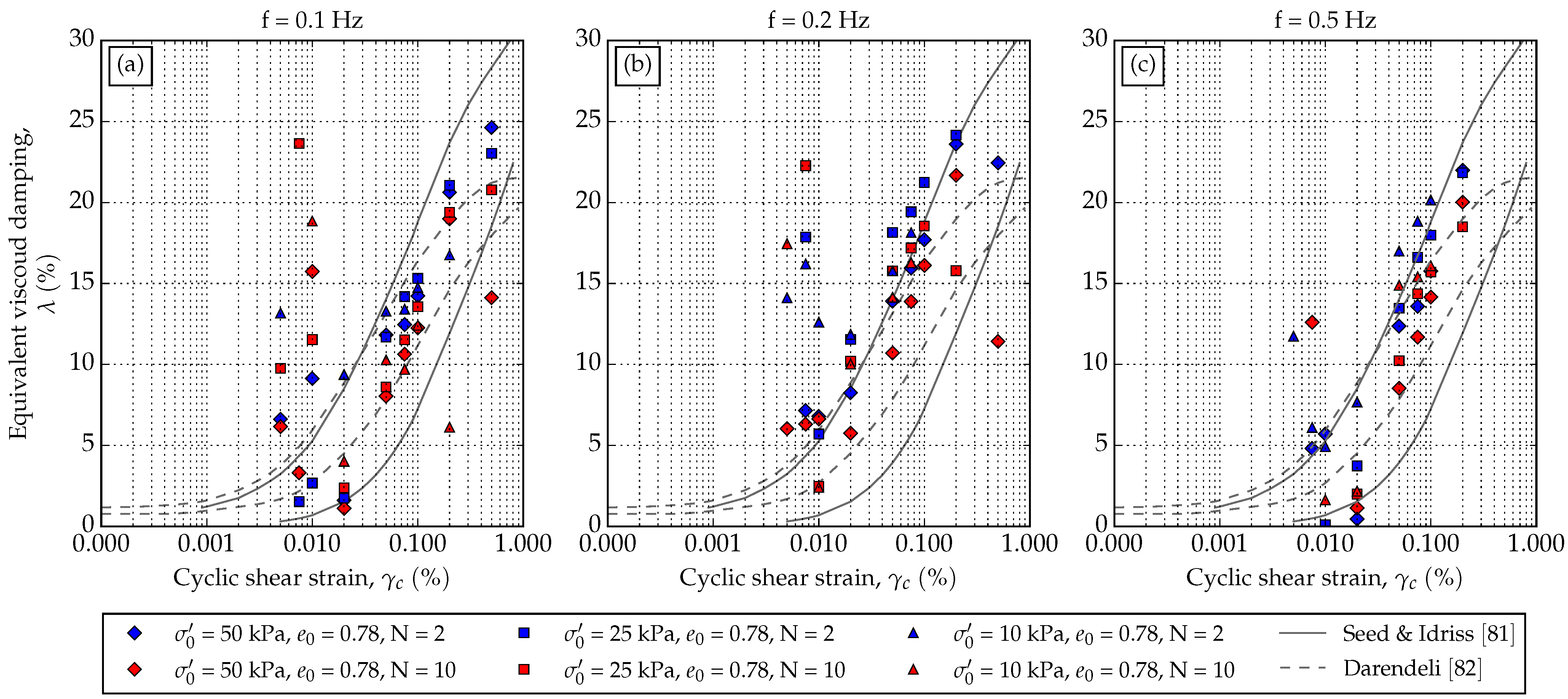
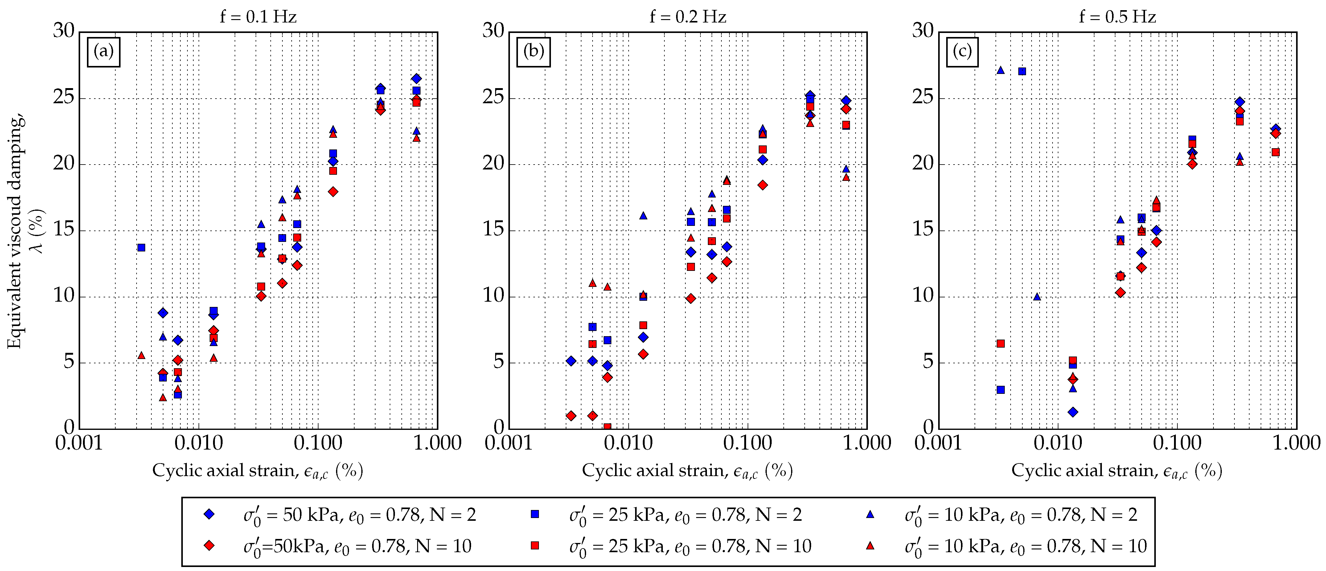
Equivalent viscous damping, $\lambda$, of uniform sand was examined in both drained and undrained conditions on dynamic triaxial equipment. Figure 8 presents the damping ratio for low confining stresses with respect to different loading frequencies (0.1, 0.2, and 0.5 Hz). Data fit well with the regions proposed by Seed and Idris [80] and Darendeli [81]. There are minor discrepancies to the fit-lines, mostly for cyclic shear strainless than 0.01%. It must be noted that the regions often used in the literature, defined by Seed and Idris [80], are for higher stress values (values higher than 80 kPa). Further, it is worth noting that the damping ratio tends to plot to the upper boundary of the Seed and Idriss regions for frequencies higher than 0.1 Hz. This scatter could also be due to the equipment used in this research. The Dynatriax system is pneumatically based and is very sensitive to system control parameters. System parameters are modified using Proportional–Integrate–Derivative (PID) [87], which can have a small impact on the measured axial strains at values lower than 0.0075%. 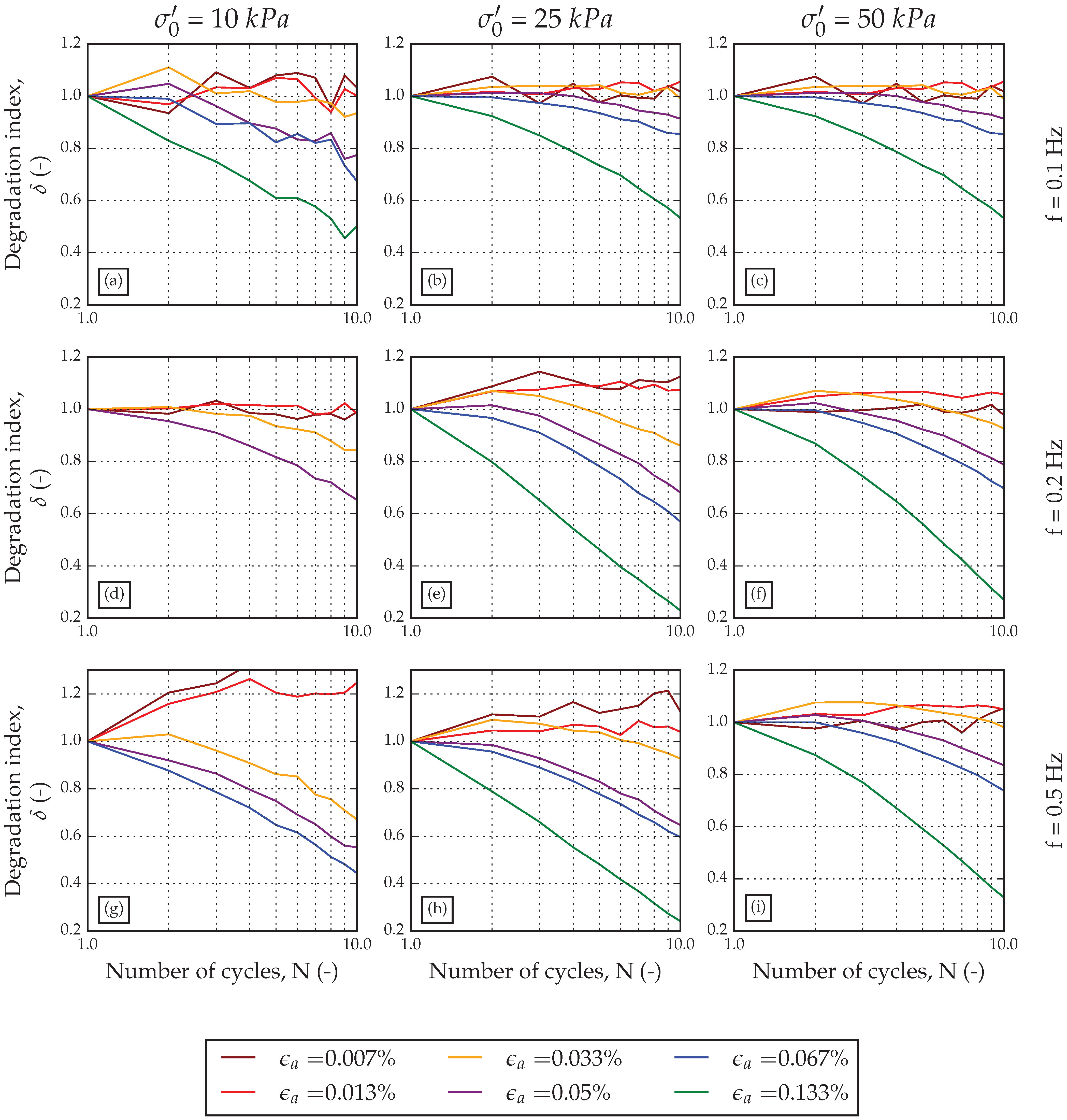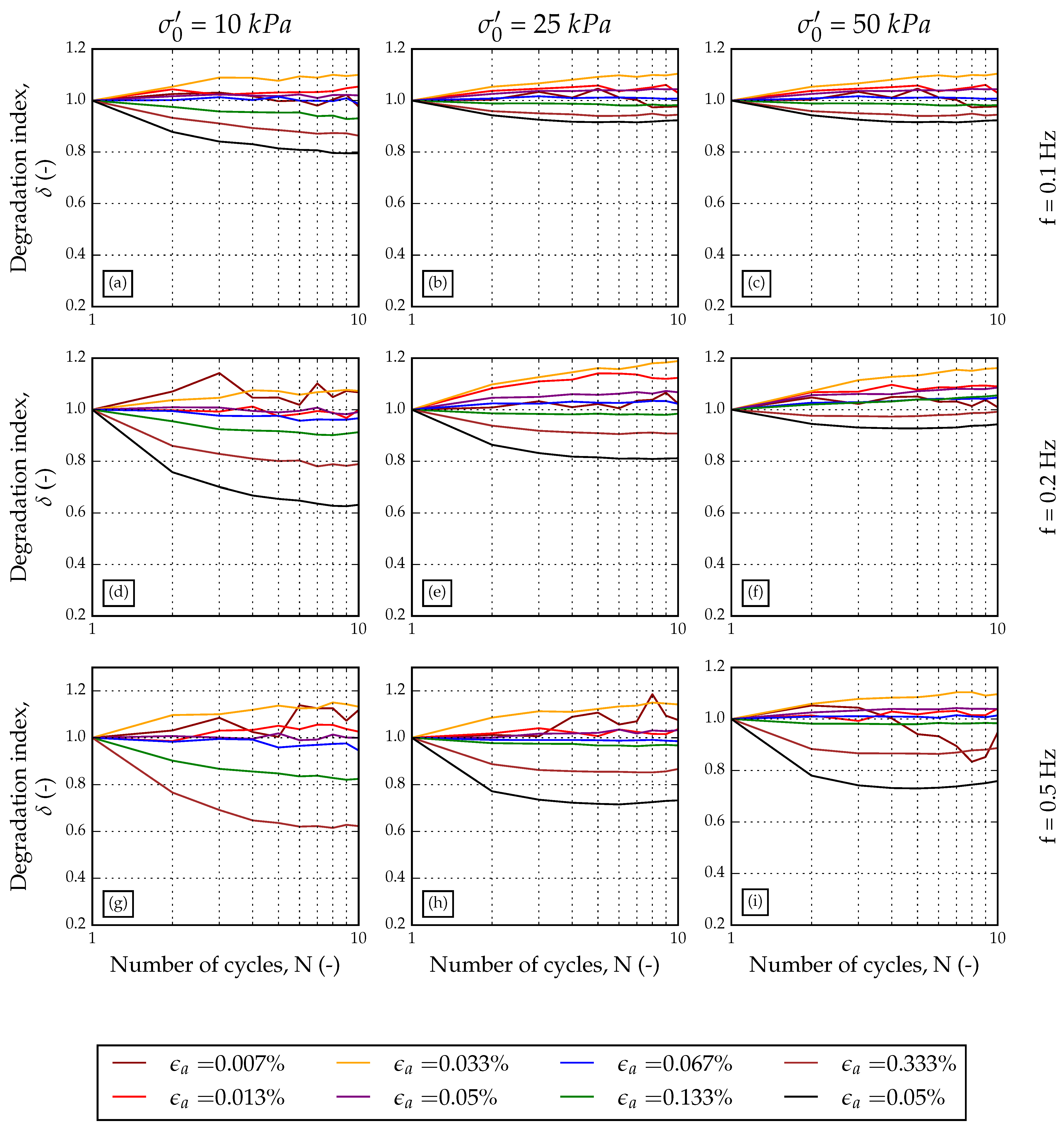Figure 9 presents the degradation index in variation with confining stresses and frequencies for undrained tests. At 0.1 Hz (Figure 9a–c), significant degradation occurs at the axial strain of 0.05%, which corresponds to the shear strain of 0.075%. The maximum degradation index is around 0.58 for confining stresses of 25 kPa and 50 kPa. As the frequency of loading increases, the soil tends to have larger degradation (lower values of the degradation index) that can be observed in the shape of the degradation curves. The influence of confining stress on the degradation index can easily be noticed at a loading frequency of 0.2 Hz (Figure 9d–f). For example, the axial strain of 0.05% has a degradation index of around 0.65 at cycle N = 10. The degradation index for confining stress of 25 kPa is around 8% higher compared to the degradation at ${\sigma }_{c,0}=10$ kPa, and around 13% lower compared to the degradation at ${\sigma }_{c,0}=50$ kPa. The degradation index shows small hardening behaviour for values of axial strain less than 0.05%. After reaching that value, degradation drops rapidly with the number of cycles. This phenomenon is well-documented behaviour for sand in cyclic simple-shear devices [48,82]. 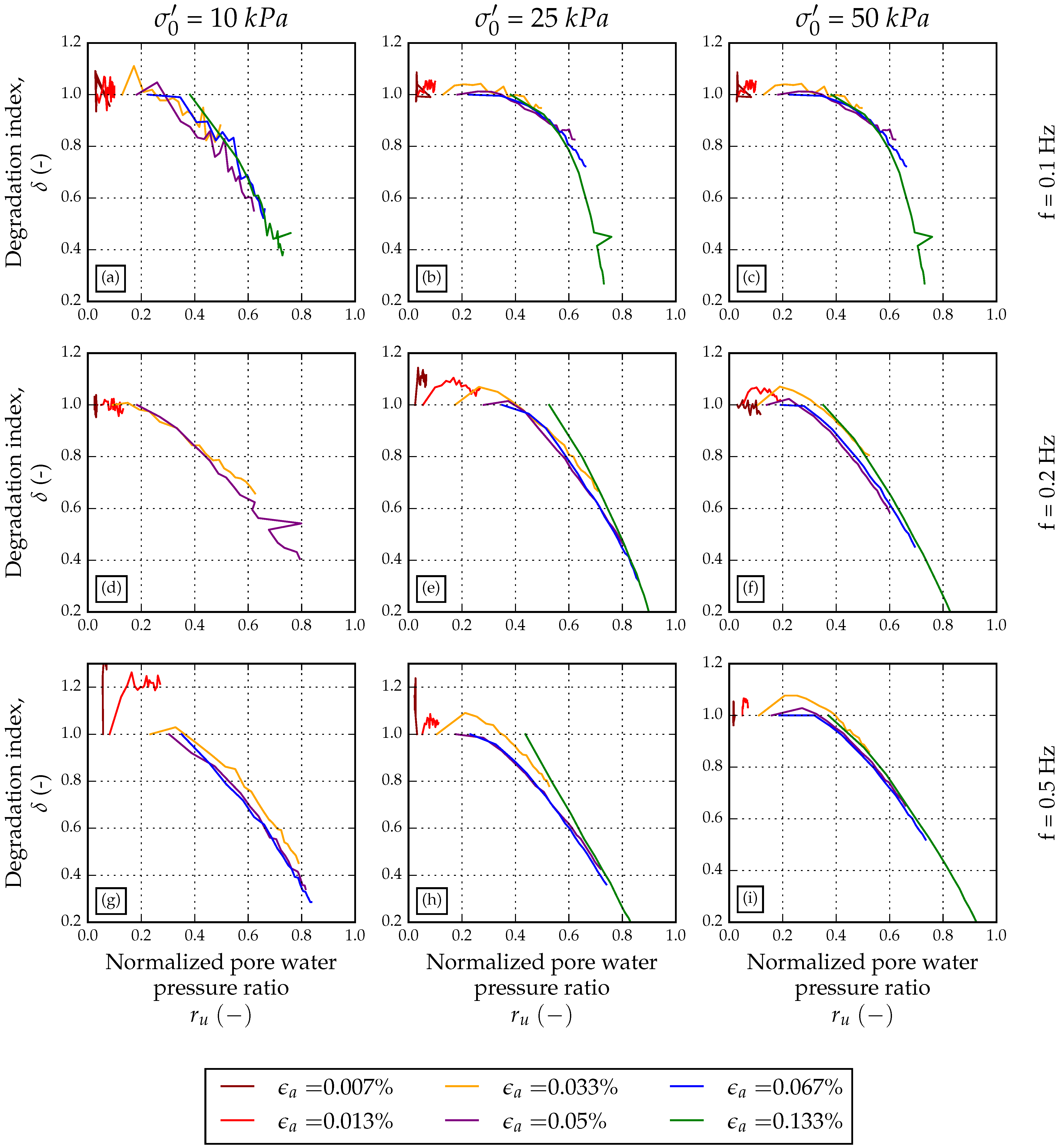To examine the correlation between the degradation index and pore water pressure, the degradation index was plotted against the normalized pore water pressure ratio (Figure 10) for various effective stresses and loading frequencies. For frequencies of 0.1 Hz and 0.2 Hz, there is rapid degradation at an effective stress of 10 kPa. For higher values of effective stress, the specimens exhibit small hardening, although the pore water pressure increases. Similar behaviour has been documented by Vucetic and Mortezaie [48]. As the confining stress becomes higher, the normalized pore water pressure ratio value for higher loading strains is lower. Figure 10e,f are presented as an example. At 0.2 Hz and axial shear strain of 0.1333%, $r_u$ for 25 kPa confining stress is around 0.5 (Figure 10e), while for 50 kPa effective confining stress it is 0.38 (Figure 10f). 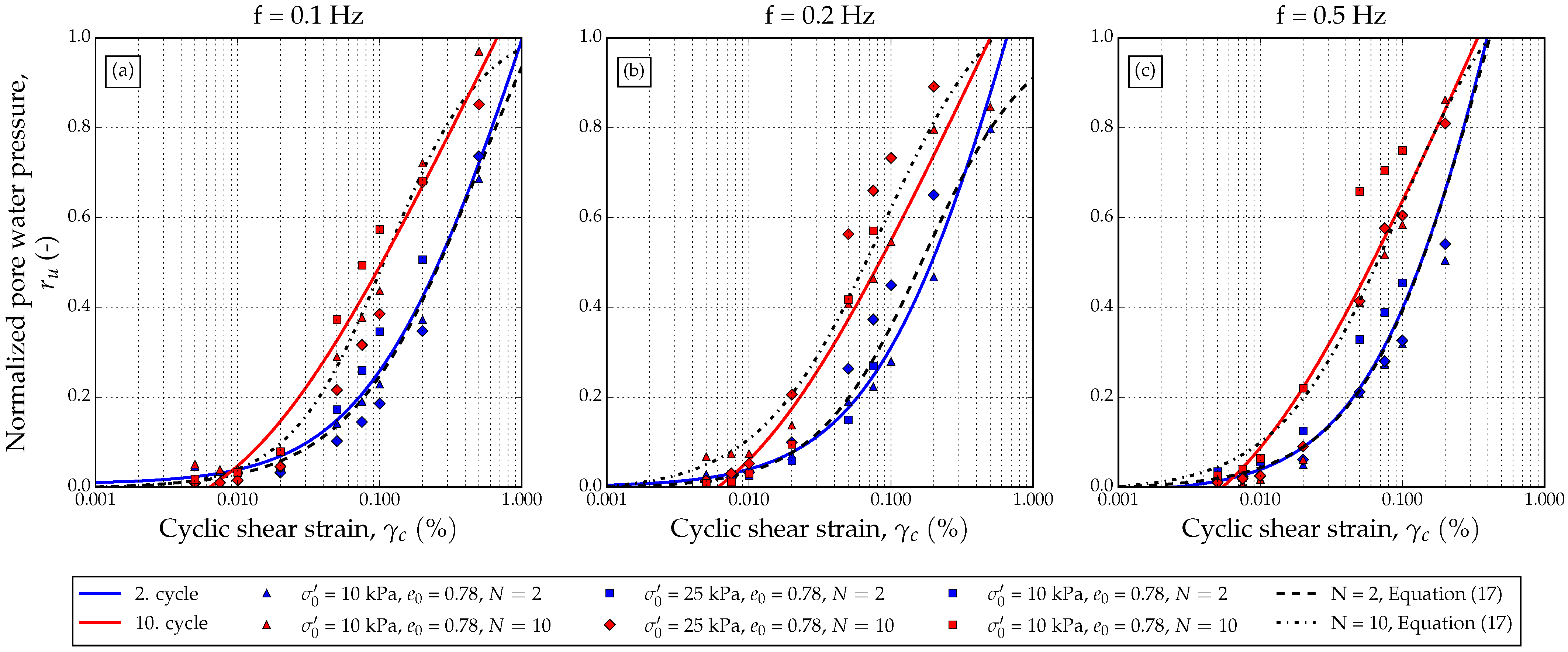These values are given for cycle N = 1. The $r_u$ values were then plotted against the equivalent cyclic shear strain with respect to the loading frequency (Figure 11). From the figure, it is evident that the pore water pressure threshold is somewhat lower than 0.01%. This is consistent with several findings in previous years [48,88]. The figure also presents the proposed simple model that takes into account the loading frequency and shearing strain. The authors suggest using Equation (15) for fast determination of the pore water pressure ratio to quickly calculate possible soil degradation. A normalized pore water pressure model proposed by Vucetic and Dobry [86] is also plotted in Figure 11. Vucetic and Dobry’s model fits well at some values of cyclic shear strain.

Drained tests focus on the result of the degradation index and volumetric strain. The authors also presented equivalent viscous damping ratios given for axial loading strain[s] (Figure 12). The increase in the equivalent viscous damping ratio has a logical trend but needs to be additionally examined at higher shearing strains.

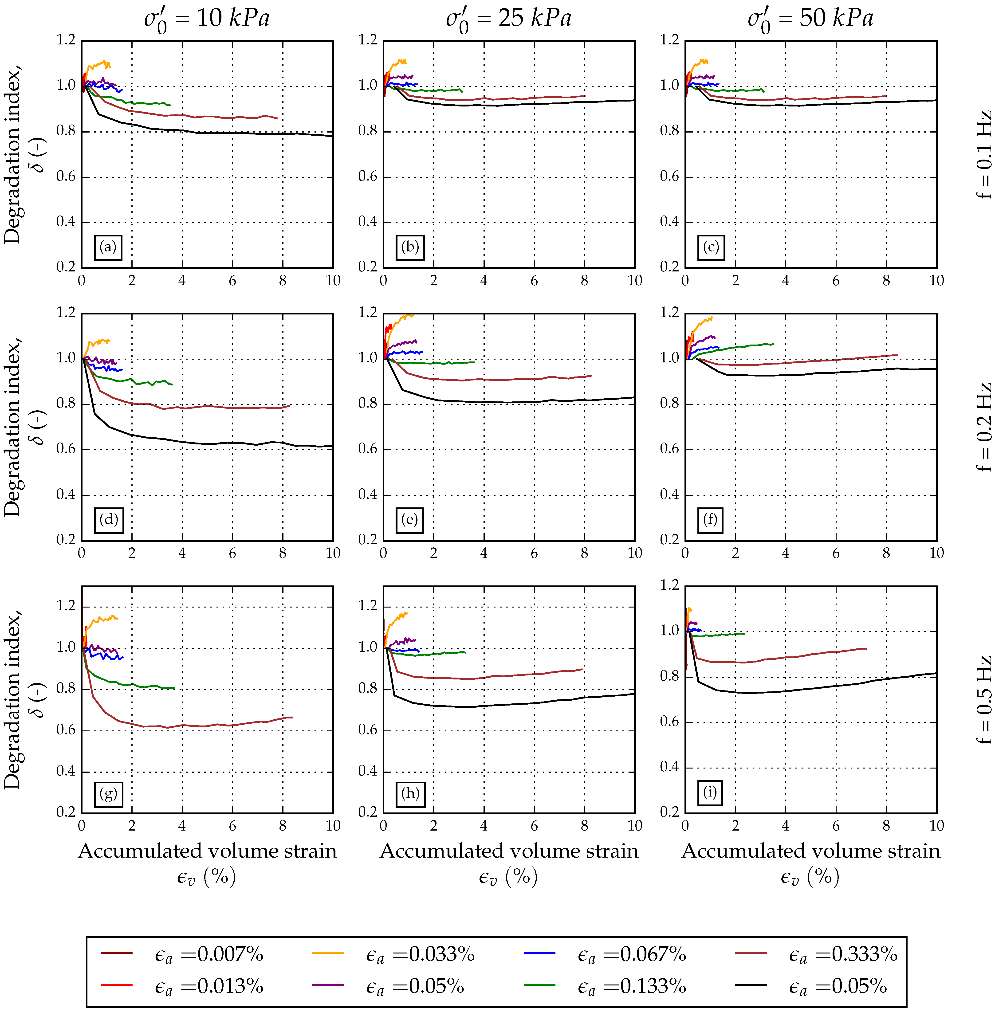
The results of the degradation index with respect to cycle number show interesting behaviour. Almost every performed test reached a loading axial strain of 0.667%, which is considered a very high loading frequency. As the confining stress rises, the degradation of the soil stops after four cycles, and in some conditions, it starts to rise. This can be interpreted to mean the soil starts to harden.

This is because in drained cyclic tests, a change in volume is allowed, and the sand densifies with the number of cycles. As the soil densifies, the average ratio of the shear modulus for a given cycle is larger than the one in the previous cycle, so the degradation index starts to rise.

This phenomenon is affected by the confining stress, as can be seen in Figure 13b–f,h,i. At low confining stress, which corresponds to Figure 13a,d,g, only degradation of sand is noticeable. The degradation index gets lower than 1 until it reaches constant value. Smaller hardening can be noticed at low axial strain loading due to dilatant soil behaviour at low cyclic strains.

Densification and hardening can be easily noticed in Figure 14, where accumulated volume strain is plotted against the degradation index. The influence of confining stresses can also be noticed in these plots, as explained earlier. For lower values of axial loading strain, there is little soil hardening, especially for low confining stresses. After several loading cycles, the volumetric strain is greatly accumulated, but degradation slowly increases. This is noticeable for the loading frequency of 0.5 Hz (Figure 14h).

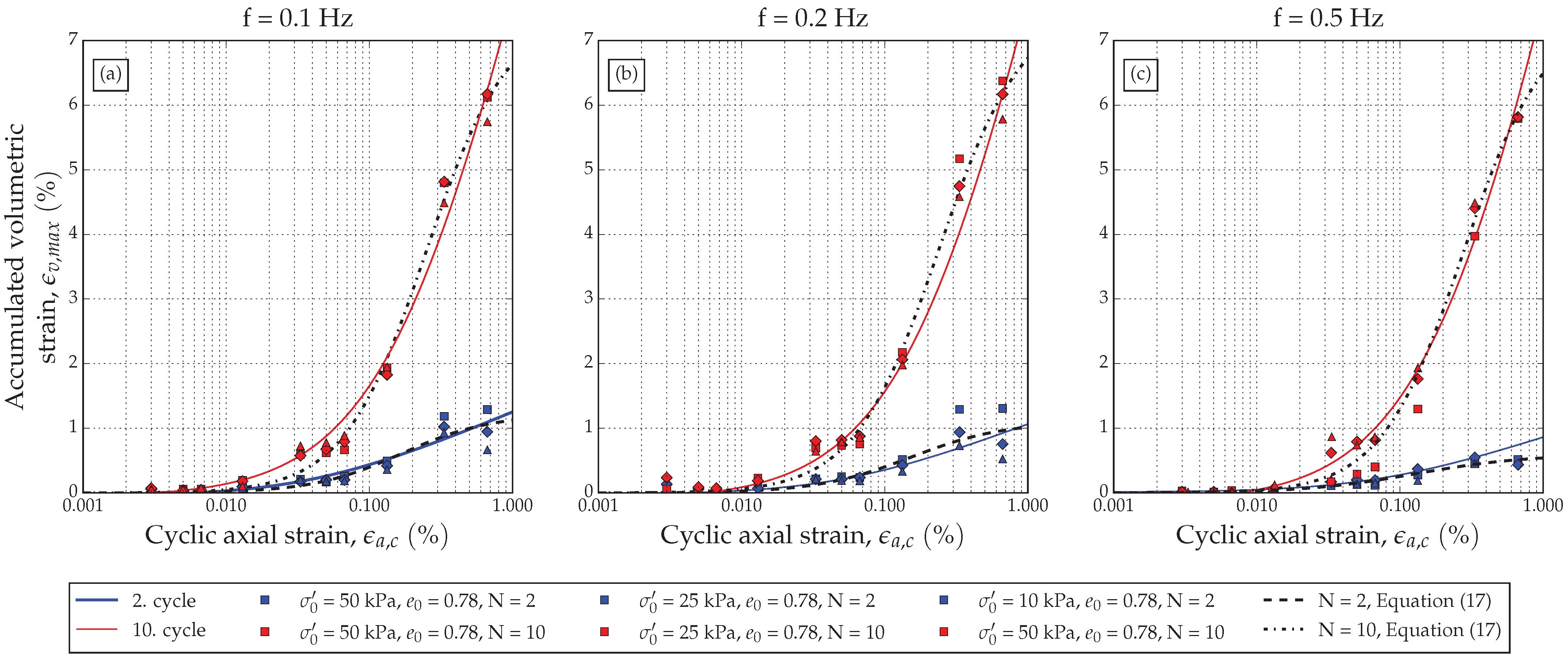
Accumulated volumetric strain is plotted against axial loading strain for cycles 2 and 10, for which simple analytical models are proposed (Equations (18) and (19)). A simple proposed model that takes into account loading frequency and axial loading strain, is presented in Figure 15. From Figure 15, it is evident that the threshold for accumulated strain is lower than 0.01% axial cyclic strain. Further worth noticing is that the accumulation of volume strain is largely affected by the number of loading cycles. This can be observed in Figure 15 as the slope of the fit curves for cycles N = 10 vs. N = 2. For comparison, data of accumulated volumetric strain are also fitted with the model proposed by Vucetic and Dobry [86], adjusted for volumetric strains and cyclic axial strains (Figure 15). As in the example of undrained data, Vucetic and Dobry’s model fits well over some range of cyclic axial strain but cannot guarantee good calculation at larger cyclic axial strains, at least not for these test results.

5. Conclusions

Low confining stresses have a large impact on the analysis of slope stability. A combination of heavy rainfall, which can fully saturate upper soil layers, with a possible post-rainfall earthquake can cause catastrophic consequences. The ongoing research project focused on the behaviour of small-scale landslide slopes at 1g conditions subjected to dynamic loading and indicated that drainage conditions and frequency also play a significant role in slope behaviour. Similarity laws for 1g conditions were used to examine the frequency of cyclic triaxial tests on uniform sand samples equivalent to prototype slope materials. Several key parameters, such as equivalent viscous damping and strength degradation, were examined and presented in this manuscript for sand in drained and undrained conditions at low confining stresses ranging from 10–50 kPa present in small-scale slope models.

From the presented results, it can be concluded that confining stress is significant for soil damping and for the degradation index in both drained and undrained conditions. Higher frequencies cause greater damping ratios. This is in common for both drained and undrained conditions.

The degradation index of tested soil showed interesting behaviour in both drained and undrained conditions. In undrained conditions, soil degrades rapidly for axial strain values that are seven times higher than the threshold value. Between the threshold strain and strain values of around 0.075%, the material first exhibits hardening and then softening, followed by significant pore water pressure build-up. For higher values of cyclic axial strain, the material needs up to five loading cycles to achieve $r_u$ of 0.65, no matter what the loading frequency is. Drained conditions showed that the material first starts to degrade after hardening takes place. This is due to soil densification that occurs as the soil compacts during cyclic loading. This means that if the water can move freely through the soil skeleton, material will degrade slightly due to volume change up to a degradation index of 0.6, but it will soon start to harden. This will beadditionally tested to examine the influence of such densification on the soil skeleton and drainage.

The proposed analytical model for the normalized pore water pressure ratio, $r_u$, related to frequency and strain, and accumulation of volumetric strain ${ϵ}_v$ related to frequency of loading and axial strain, show very good fit to the tested results. These analytical models can help to quickly calculate the pore water pressure and/or volumetric strain for this type of material considering low confining stresses. The proposed model is compared to the model proposed by Vucetic and Dobry [86] and can better evaluate the pore pressure and volumetric changes in conditions of low confining stress. This is important because low confining stress presents a governing factor for the behaviour of shallow landslides and for 1g conditions that exist in models areof small dimensions, such as small-scale landslide models. The proposed analytical models can simply be used to determine the pore pressure ratio values for small-scale slope models subjected to dynamic loading, such as earthquakes.

As a part of ongoing research on landslide activation at 1g conditions subjected to dynamic loading to determine slope behaviour [22], the results presented in this manuscript show specific behaviour of sand that needs to be taken into consideration when the behaviour of a landslide in a model is analysed.

The main limitations of the study lay in limited use of proposed models to uniform, sandy soils and loading frequencies of 0.5 Hz, corresponding to maximal values used in small-scale slope testing on a shaking table. For other soil materials, especially those with higher content of fine particles, additional triaxial tests should be conducted using the procedures described in this manuscript.

To summarize:

• Low confining stress plays a significant role in the dynamic properties of sand in both drained and undrained conditions.
• In undrained tests, for axial strains up to $0.033\%$, sand first hardens and then degrades. At higher values of strain, it only degrades.
• In undrained tests, for axial strains up to $0.033\%$, sand generates up to 40% $r_u$, but it does not have a significant effect on degradation. At higher values of strain, $r_u$ rapidly rises.
• In drained tests, degradation decreases after the fourth cycle for larger values of confining stress. After the fourth cycle, soil densifies due to accumulated volumetric strain.
• In drained tests, degradation after the fourth cycle decreases and hardening takes place.
• The proposed analytical models for $r_u$ and ${\epsilon }_v$ are in good correlation to the tested results and can be used to evaluate the normalized pore water pressure ratio and/or accumulated volumetric strains for cycles N = 2 or N = 10 in conditions of low confining stress.

References

1. Popescu, M.E. Landslide causal factors and landslide remediatial options. In Proceedings of the 3rd International Conference on Landslides, Slope Stability and Safety of Infra-Structures, Singapore, 11–12 July 2002; pp. 61–81. [Google Scholar]
2. Wu, L.Z.; Huang, R.Q.; Xu, Q.; Zhang, L.M.; Li, H.L. Analysis of physical testing of rainfall-induced soil slope failures. Environ. Earth Sci. 2015, 73, 8519–8531. [Google Scholar] [CrossRef]
3. Kumar, S.S.; Krishna, A.M.; Dey, A. Evaluation of dynamic properties of sandy soil at high cyclic strains. Soil Dyn. Earthq. Eng. 2017, 99, 157–167. [Google Scholar] [CrossRef]
4. Icl. Instruction for World Reports on Landslides; Technical Report; Icl: New York, NY, USA, 2016. [Google Scholar]
5. Yang, J.; Luo, X. Exploring the relationship between critical state and particle shape for granular materials. J. Mech. Phys. Solids 2015, 84, 196–213. [Google Scholar] [CrossRef]
6. Gabet, E.J.; Mudd, S.M. The mobilization of debris flows from shallow landslides. Geomorphology 2006, 74, 207–218. [Google Scholar] [CrossRef]
7. Iida, T. Theoretical research on the relationship between return period of rainfall and shallow landslides. Hydrol. Process. 2004, 18, 739–756. [Google Scholar] [CrossRef]
8. Saito, H.; Nakayama, D.; Matsuyama, H. Two Types of Rainfall Conditions Associated with Shallow Landslide Initiation in Japan as Revealed by Normalized Soil Water Index. SOLA 2010, 6, 57–60. [Google Scholar] [CrossRef] [Green Version]
9. Matsushi, Y.; Hattanji, T.; Matsukura, Y. Mechanisms of shallow landslides on soil-mantled hillslopes with permeable and impermeable bedrocks in the Boso Peninsula, Japan. Geomorphology 2006, 76, 92–108. [Google Scholar] [CrossRef]
10. Saito, H.; Nakayama, D.; Matsuyama, H. Relationship between the initiation of a shallow landslide and rainfall intensity-duration thresholds in Japan. Geomorphology 2010, 118, 167–175. [Google Scholar] [CrossRef]
11. Gariano, S.L.; Brunetti, M.T.; Iovine, G.; Melillo, M.; Peruccacci, S.; Terranova, O.; Vennari, C.; Guzzetti, F. Calibration and validation of rainfall thresholds for shallow landslide forecasting in Sicily, southern Italy. Geomorphology 2015, 228, 653–665. [Google Scholar] [CrossRef]
12. Salciarini, D.; Godt, J.W.; Savage, W.Z.; Conversini, P.; Baum, R.L.; Michael, J.A. Modeling regional initiation of rainfall-induced shallow landslides in the eastern Umbria Region of central Italy. Landslides 2006, 3, 181–194. [Google Scholar] [CrossRef]
13. Giannecchini, R.; Galanti, Y.; D’Amato Avanzi, G. Critical rainfall thresholds for triggering shallow landslides in the Serchio River Valley (Tuscany, Italy). Nat. Hazards Earth Syst. Sci. 2012, 12, 829–842. [Google Scholar] [CrossRef]
14. Vennari, C.; Gariano, S.L.; Antronico, L.; Brunetti, M.T.; Iovine, G.; Peruccacci, S.; Terranova, O.; Guzzetti, F. Rainfall thresholds for shallow landslide occurrence in Calabria, southern Italy. Nat. Hazards Earth Syst. Sci. 2014, 14, 317–330. [Google Scholar] [CrossRef] [Green Version]
15. Arbanas, Ž.; Sassa, K.; Nagai, O.; Jagodnik, V.; Vivoda, M.; Jovančevic, S.D.; Perani c, J.; Ljuti c, K. A Landslide Monitoring and Early Warning System Using Integration of GPS, TPS and Conventional Geotechnical Monitoring Methods; Springer: Berlin/Heidelberg, Germany, 2014; pp. 631–636. [Google Scholar] [CrossRef]
16. Pecoraro, G.; Calvello, M.; Piciullo, L. Monitoring strategies for local landslide early warning systems. Landslides 2019, 16, 213–231. [Google Scholar] [CrossRef]
17. Guzzetti, F.; Gariano, S.L.; Peruccacci, S.; Brunetti, M.T.; Marchesini, I.; Rossi, M.; Melillo, M. Geographical landslide early warning systems. Earth-Sci. Rev. 2020, 200, 102973. [Google Scholar] [CrossRef]
18. Stark, T.D.; Choi, H.; McCone, S. Drained Shear Strength Parameters for Analysis of Landslides. J. Geotech. Geoenviron. Eng. 2005, 131, 575–588. [Google Scholar] [CrossRef]
19. Öge, İ.F. Investigation of design parameters of a failed soil slope by back analysis. Eng. Fail. Anal. 2017, 82, 266–279. [Google Scholar] [CrossRef]
20. Donati, D.; Stead, D.; Brideau, M.A.; Ghirotti, M. Using pre-failure and post-failure remote sensing data to constrain the three-dimensional numerical model of a large rock slope failure. Landslides 2021, 18, 827–847. [Google Scholar] [CrossRef]
21. Chen, X.P.; Liu, D. Residual strength of slip zone soils. Landslides 2014, 11, 305–314. [Google Scholar] [CrossRef]
22. Arbanas, Ž.; Pajalić, S.; Jagodnik, V.; Peranić, J.; Vivoda Prodan, M.; Domlija, P.; Dugonjić-Jovančević, S. Development of physical model of landslide remedial constructions’ behaviour. In Proceedings of the 4th Regional Symposium on Landslides in the Adriatic-Balkan Region, Sarajevo, Bosnia and Herzegovina, 23–25 October 2019; Uljarević, M., Zekan, S., Salković, S., Ibrahimović, D., Eds.; Društvo za Geotehniku u Bosni i Hercegovini: Sarajevo, Bosnia and Herzegovina, 2019; pp. 103–108. [Google Scholar] [CrossRef]
23. Pajalić, S.; Peranić, J.; Maksimović, S.; Čeh, N.; Jagodnik, V.; Arbanas, Ž. Monitoring and data analysis in small-scale landslide physical model. Appl. Sci. 2021, 11, 5040. [Google Scholar] [CrossRef]
24. Jagodnik, V.; Turković, M.; Arbanas, Ž. Preliminary results on the undrained cyclic behavior of uniform sand at low confining stress. In Proceedings of the 5th Regional Symposium on Landslides in the Adriatic-Balkan Region, Rijeka, Croatia, 23–26 March 2022; Peranić, J., Vivoda Prodan, M., Bernat Gazibara, S., Krkač, M., Mihalič Arbanas, S., Arbanas, Ž., Eds.; Faculty of Civil Engineering, University of Rijeka and Faculty of Mining, Geology and Petroleum Engineering, University of Zagreb: Rijeka, Croatia, 2022; pp. 201–206. [Google Scholar]
25. Yang, G.; Qi, S.; Wu, F.; Zhan, Z. Seismic amplification of the anti-dip rock slope and deformation characteristics: A large-scale shaking table test. Soil Dyn. Earthq. Eng. 2018, 115, 907–916. [Google Scholar] [CrossRef]
26. Jafarzadeh, F.; Farahi-Jahromi, H.; Rajabigol, M. Applicability of rigid block based approaches in predicting sandy slope displacements by 1g shaking table tests. Soil Dyn. Earthq. Eng. 2019, 126, 105576. [Google Scholar] [CrossRef]
27. Wang, K.L.; Lin, M.L. Initiation and displacement of landslide induced by earthquake—A study of shaking table model slope test. Eng. Geol. 2011, 122, 106–114. [Google Scholar] [CrossRef]
28. Wartman, J.; Seed, R.B.; Bray, J.D. Shaking Table Modeling of Seismically Induced Deformations in Slopes. J. Geotech. Geoenviron. Eng. 2005, 131, 610–622. [Google Scholar] [CrossRef]
29. Ozkahriman, F.; Wartman, J. Investigation of 1-G Similitude Laws by “Modeling-of-Models” Exercise; American Society of Civil Engineers: Reston, VA, USA, 2007. [Google Scholar] [CrossRef]
30. Grasso, S.; Lentini, V.; Sammito, M.S.V. A New Biaxial Laminar Shear Box for 1 g Shaking Table Tests on Liquefiable Soils. In Geotechnical, Geological and Earthquake Engineering; Springer: Cham, Switzerland, 2022; pp. 1499–1507. [Google Scholar] [CrossRef]
31. Ling, H.; Ling, H.I. Centrifuge Model Simulations of Rainfall-Induced Slope Instability. J. Geotech. Geoenviron. Eng. 2012, 138, 1151–1157. [Google Scholar] [CrossRef]
32. Zhang, Z.; Wang, T.; Wu, S.; Tang, H.; Liang, C. Seismic performance of loess-mudstone slope by centrifuge tests. Bull. Eng. Geol. Environ. 2017, 76, 671–679. [Google Scholar] [CrossRef]
33. Zhang, Z.; Wang, T.; Wu, S.; Tang, H.; Liang, C. Investigation of dormant landslides in earthquake conditions using a physical model. Landslides 2017, 14, 1181–1193. [Google Scholar] [CrossRef]
34. Take, W.A.; Bolton, M.D.; Wong, P.C.P.; Yeung, F.J. Evaluation of landslide triggering mechanisms in model fill slopes. Landslides 2004, 1, 173–184. [Google Scholar] [CrossRef]
35. Wang, S.; Idinger, G.; Wu, W. Centrifuge modelling of rainfall-induced slope failure in variably saturated soil. Acta Geotech. 2021, 16, 2899–2916. [Google Scholar] [CrossRef]
36. Matziaris, V.; Marshall, A.M.; Yu, H.S. Centrifuge Model Tests of Rainfall-Induced Landslides. In Recent Advances in Modeling Landslides and Debris Flows; Wu, W., Ed.; Springer: Cham, Switzerland, 2015; pp. 73–83. [Google Scholar] [CrossRef]
37. Madabhushi, G. Centrifuge Modelling for Civil Engineers; CRC Press: Boca Raton, FL, USA, 2017. [Google Scholar]
38. Eckersley, D. Instrumented laboratory flowslides. Géotechnique 1990, 40, 489–502. [Google Scholar] [CrossRef]
39. Clough, R.W.; Pirtz, D. Earthquake Resistance of Rock-Fill Dams. J. Soil Mech. Found. Div. 1956, 82, 1–26. [Google Scholar] [CrossRef]
40. Fan, G.; Zhang, J.; Wu, J.; Yan, K. Dynamic Response and Dynamic Failure Mode of a Weak Intercalated Rock Slope Using a Shaking Table. Rock Mech. Rock Eng. 2016, 49, 3243–3256. [Google Scholar] [CrossRef]
41. Lin, M.L.; Wang, K.L. Seismic slope behavior in a large-scale shaking table model test. Eng. Geol. 2006, 86, 118–133. [Google Scholar] [CrossRef]
42. Jibson, R.W. Methods for assessing the stability of slopes during earthquakes—A retrospective. Eng. Geol. 2011, 122, 43–50. [Google Scholar] [CrossRef]
43. Iai, S.; Tobita, T.; Nakahara, T. Generalised scaling relations for dynamic centrifuge tests. Geotechnique 2005, 55, 355–362. [Google Scholar] [CrossRef]
44. White, J.R.F. A Laboratory Investigation into the Behaviour of Sand at Low Confining Stresses; University of Oxford: Oxford, UK, 2020. [Google Scholar]
45. Dobry, R.; Ladd, R.; Yokel, F.Y.; Chung, R.M.; Powell, D. Prediction of Pore Water Pressure Buildup and Liquefaction of Sands during Earthquakes by the Cyclic Strain Method; National Bureau of Standards: Gaithersburg, MD, USA, 1982; Volume 138. [Google Scholar]
46. Vucetic, M. Cyclic Threshold Shear Strains in Soils. J. Geotech. Eng. 1994, 120, 2208–2228. [Google Scholar] [CrossRef]
47. Tabata, K.; Vucetic, M. Threshold Shear Strain for Cyclic Degradation of Three Clays. In Proceedings of the 5th International Conferences on Recent Advances in Geotechnical Earthquake Engineering and Soil Dynamics, Missouri University of Science and Technology, Rolla, MO, USA, 24–29 May 2010; p. 30. [Google Scholar]
48. Vucetic, M.; Mortezaie, A. Cyclic secant shear modulus versus pore water pressure in sands at small cyclic strains. Soil Dyn. Earthq. Eng. 2015, 70, 60–72. [Google Scholar] [CrossRef] [Green Version]
49. Chakraborty, T.; Salgado, R. Dilatancy and Shear Strength of Sand at Low Confining Pressures. J. Geotech. Geoenviron. Eng. 2010, 136, 527–532. [Google Scholar] [CrossRef]
50. Shaoli, Y.; Sandven, R.; Grande, L. Liquefaction of sand under low confining pressure. J. Ocean Univ. Qingdao 2003, 2, 207–210. [Google Scholar] [CrossRef]
51. Sture, S.; Batiste, S.; Lankton, M.; Parisi, J. Properties of Sand under Low Effective Stresses. In Proceedings of the Ninth Biennial Conference on Engineering, Construction, and Operations in Challenging Environments, League City, Houston, TX, USA, 7–10 March 2004; Ramesh, B., Malla, R., Maji, A., Eds.; American Society of Civil Engineers: Reston, VA, USA, 2004; pp. 78–84. [Google Scholar] [CrossRef]
52. NASA. What Is Microgravity? Available online: https://www.nasa.gov/audience/forstudents/5-8/features/nasa-knows/what-is-microgravity-58.html (accessed on 2 September 2022).
53. Lee, C.T.; Huang, C.C.; Lee, J.F.; Pan, K.L.; Lin, M.L.; Dong, J.J. Statistical approach to earthquake-induced landslide susceptibility. Eng. Geol. 2008, 100, 43–58. [Google Scholar] [CrossRef]
54. Lee, S.; Evangelista, D.G. Earthquake-induced landslide-susceptibility mapping using an artificial neural network. Nat. Hazards Earth Syst. Sci. 2006, 6, 687–695. [Google Scholar] [CrossRef]
55. Umar, Z.; Pradhan, B.; Ahmad, A.; Jebur, M.N.; Tehrany, M.S. Earthquake induced landslide susceptibility mapping using an integrated ensemble frequency ratio and logistic regression models in West Sumatera Province, Indonesia. CATENA 2014, 118, 124–135. [Google Scholar] [CrossRef]
56. Glade, T.; Nadim, F. Early warning systems for natural hazards and risks. Nat. Hazards 2014, 70, 1669–1671. [Google Scholar] [CrossRef] [Green Version]
57. Ma, J.; Xia, D.; Guo, H.; Wang, Y.; Niu, X.; Liu, Z.; Jiang, S. Metaheuristic-based support vector regression for landslide displacement prediction: A comparative study. Landslides 2022, 19, 2489–2511. [Google Scholar] [CrossRef]
58. Ma, J.; Xia, D.; Wang, Y.; Niu, X.; Jiang, S.; Liu, Z.; Guo, H. A comprehensive comparison among metaheuristics (MHs) for geohazard modeling using machine learning: Insights from a case study of landslide displacement prediction. Eng. Appl. Artif. Intell. 2022, 114, 105150. [Google Scholar] [CrossRef]
59. Miranda, E.; Brzev, S.; Bijelić, N.; Arbanas, Ž.; Bartolac, M.; Jagodnik, V.; Lazarević, D.; Arbanas, S.M.; Zlatović, S.; Acosta, A.; et al. StEER-EERI: Petrinja, Croatia December 29, 2020, Mw 6.4 Earthquake Joint Reconnaissance Report (JRR). 2021. Available online: https://www.designsafe-ci.org/data/browser/public/designsafe.storage.published/PRJ-2959/details-4541797621822058005-242ac118-0001-012 (accessed on 2 September 2022).
60. Herak, D.; Sović, I.; Cecić, I.; Živčić, M.; Dasović, I.; Herak, M. Historical seismicity of the Rijeka region (northwest External Dinarides, Croatia)—Part I: Earthquakes of 1750, 1838, and 1904 in the Bakar epicentral area. Seismol. Res. Lett. 2017, 88, 904–915. [Google Scholar] [CrossRef]
61. Herak, M.; Živčić, M.; Sović, I.; Cecić, I.; Dasović, I.; Stipčević, J.; Herak, D. Historical Seismicity of the Rijeka Region (Northwest External Dinarides, Croatia)—Part II: The Klana Earthquakes of 1870. Seismol. Res. Lett. 2018, 89, 1524–1536. [Google Scholar] [CrossRef]
62. Quanser. Shake Table III XY Data Sheet; Quanser: Markham, ON, Canada, 2022. [Google Scholar]
63. Han, R.; Zhao, X. Shaking Table Tests and Validation of Multi-Modal Sensing and Damage Detection Using Smartphones. Buildings 2021, 11, 477. [Google Scholar] [CrossRef]
64. Larbi, S.H.; Bourahla, N.; Benchoubane, H.; Choutri, K.; Badaoui, M. Earthquake Ground Motion Matching on a Small Electric Shaking Table Using a Combined NN-PDFF Controller. Shock Vib. 2020, 2020, 7260590. [Google Scholar] [CrossRef]
65. Bićanić, N.; Camenen, J.F.; Čeh, N.; Koziara, T. Characterisation of pattern formation in constrained multiblock assembly subjected to horizontal harmonic excitation. Int. J. Mason. Res. Innov. 2016, 1, 375. [Google Scholar] [CrossRef]
66. Dobrilla, S.; Čeh, N.; Tuhtan, M.; Jelenić, G. Experimental Analysis of Structure Response to Non-uniform Support Excitation. Zb. Rad. 2018, 20, 175–188. [Google Scholar] [CrossRef] [Green Version]
67. Controls. Dynamic Triaxial System—DYNATRIAX Testing Equipment, Controls. Available online: https://www.controls-group.com/usa/dynamic-testing-systems/dynamic-triaxial-system-dynatriax-ems.php (accessed on 31 August 2020).
68. ISO 14688-1:2017; Geotechnical Investigation and Testing—Identification and Classification of Soil—Part 1: Identification and Description. Technical Report; ISO: Geneva, Switzerland, 2017.
69. Ladd, R.S. Preparing test specimens using under compaction. Geotech. Test. J. 1978, 1, 16–23. [Google Scholar] [CrossRef]
70. Kodicherla, S.P.K.; Gong, G.; Fan, L.; Moy, C.K.; He, J. Effects of preparation methods on inherent fabric anisotropy and packing density of reconstituted sand. Cogent Eng. 2018, 5, 1533363. [Google Scholar] [CrossRef]
71. Frost, J.D.; Park, J.Y. A critical assessment of the moist tamping technique. Geotech. Test. J. 2003, 26, 57–70. [Google Scholar] [CrossRef]
72. Raghunandan, M.E.; Juneja, A.; Hsiung, B.C.B. Preparation of reconstituted sand samples in the laboratory. Int. J. Geotech. Eng. 2012, 6, 125–131. [Google Scholar] [CrossRef]
73. da Fonseca, A.V.; Cordeiro, D.; Molina-Gómez, F. Recommended Procedures to Assess Critical State Locus from Triaxial Tests in Cohesionless Remoulded Samples. Geotechnics 2021, 1, 95–127. [Google Scholar] [CrossRef]
74. Lade, P.V. Triaxial Testing of Soils; Wiley: Hoboken, NJ, USA, 2016. [Google Scholar] [CrossRef]
75. Wood, D.M. Soil Behaviour and Critical State Soil Mechanics; Cambridge University Press: Cambridge, UK, 1990. [Google Scholar]
76. Duncan, J.M.; Seed, H.B. Errors in Strength Tests and Recommended Corrections; Technical Report; California University Berkeley Institute of Transportation and Traffic Engineering: Berkeley, CA, USA, 1965. [Google Scholar]
77. Duncan, J.M.; Seed, H.B. Corrections for strength test data. J. Soil Mech. Found. Div. 1967, 93, 121–137. [Google Scholar] [CrossRef]
78. Silver, M.L.; Seed, H.B. Volume Changes in Sands during Cyclic Loading. J. Soil Mech. Found. Div. 1971, 97, 1171–1182. [Google Scholar] [CrossRef]
79. Thian, S.; Lee, C. Cyclic stress-controlled tests on offshore clay. J. Rock Mech. Geotech. Eng. 2017, 9, 376–381. [Google Scholar] [CrossRef]
80. Seed, H.B.; Idriss, I.M. Soil Moduli and Damping Factors for Dynamic Response Analyses; Technical Report; Earthquake Engineering Research Center, University of California: Berkeley, CA, USA, 1970. [Google Scholar]
81. Darendeli, M.B. A New Family of Normalized Modulus Reduction and Material Damping Curves. Ph.D. Thesis, University of Texas, Austin, TX, USA, 2001; p. 362. [Google Scholar]
82. Vucetic, M.; Thangavel, H.; Mortezaie, A. Cyclic Secant Shear Modulus and Pore Water Pressure Change in Sands at Small Cyclic Strains. J. Geotech. Geoenviron. Eng. 2021, 147, 04021018. [Google Scholar] [CrossRef]
83. Van Rossum, G.; Drake, F.L. Python 3 Reference Manual; CreateSpace: Scotts Valley, CA, USA, 2009. [Google Scholar]
84. Virtanen, P.; Gommers, R.; Oliphant, T.E.; Haberland, M.; Reddy, T.; Cournapeau, D.; Burovski, E.; Peterson, P.; Weckesser, W.; Bright, J.; et al. SciPy 1.0: Fundamental algorithms for scientific computing in Python. Nat. Methods 2020, 17, 261–272. [Google Scholar] [CrossRef] [Green Version]
85. Vinet, L.; Zhedanov, A. A ‘Missing’ Family of Classical Orthogonal Polynomials. In Scientific Computation; Springer: Dordrecht, The Netherlands; New York, NY, USA, 2011; Volume 44, p. 366. [Google Scholar] [CrossRef]
86. Vucetic, M.; Dobry, R. Pore Pressure Build-Up and Liquefaction at Level Sandy Sites during Earthquakes; Technical Report, CE-86-3; Rensselaer Polytechnic Institute: Troy, NY, USA, 1986. [Google Scholar]
87. Panda, R.C. Introduction to PID Controllers: Theory, Tuning and Application to Frontier Areas; InTech: Rijeka, Croatia, 2012. [Google Scholar]
88. Mortezaie, A.; Vucetic, M. Threshold Shear Strains for Cyclic Degradation and Cyclic Pore Water Pressure Generation in Two Clays. J. Geotech. Eng. 2016, 142, 1–14. [Google Scholar] [CrossRef]
Figure 1. Flowchart of shallow landslide examination process: (a) geotechnical model input, (b) type of model decision, (c) numerical model, (d) physical model, (e) static and cyclic laboratory results, and (f) verification of numerical and/or physical models.
Sustainability 14 12797 g001
Figure 2. Schematic view of slope models used in simulations: (a) prototype of slope with potential for shallow landslide, and (b) small-scale model used for dynamic loading test.
Sustainability 14 12797 g002
Figure 3. Small-scale landslide under dynamic loading: (a) prepared test, and (b) dynamically induced landslide.
Sustainability 14 12797 g003
Figure 4. Cyclic triaxial system: (a) water tank, (b) pneumatic actuator, (c) triaxial loading frame, (d) triaxial cell, (e) volume controller, (f) PC with data acquisition system, (g) pneumatic control system for pressures and actuator, and (h) water distribution panel, according to [24].
Sustainability 14 12797 g004
Figure 5. Grain-size distribution curve of Drava sand.
Sustainability 14 12797 g005
Figure 6. Sample preparation using undercompaction method: (a) lower layers of compaction, and (b) upper layers of compaction, according to [24].
Sustainability 14 12797 g006
Figure 7. Non-symmetrical cyclic triaxial loop used for equivalent viscous damping calculation.
Sustainability 14 12797 g007
Figure 8. Equivalent viscous damping ratio according to used frequency: (a) 0.1 Hz loading frequency, (b) 0.2 Hz loading frequency, and (c) 0.5 Hz loading frequency.
Sustainability 14 12797 g008
Figure 9. Degradation index related to number of cycles: (a) 0.1 Hz loading frequency at confining stress of 10 kPa, (b) 0.1 Hz loading frequency at confining stress of 25 kPa, (c) 0.1 Hz loading frequency at confining stress of 50 kPa, (d) 0.2 Hz loading frequency at confining stress of 10 kPa, (e) 0.2 Hz loading frequency at confining stress of 25 kPa, (f) 0.2 Hz loading frequency at confining stress of 50 kPa, (g) 0.5 Hz loading frequency at confining stress of 10 kPa, (h) 0.5 Hz loading frequency at confining stress of 25 kPa, and (i) 0.5 Hz loading frequency at confining stress of 50 kPa.
Sustainability 14 12797 g009
Figure 10. Degradation index related to normalised pore water pressure ratio: (a) 0.1 Hz loading frequency at confining stress of 10 kPa, (b) 0.1 Hz loading frequency at confining stress of 25 kPa, (c) 0.1 Hz loading frequency at confining stress of 50 kPa, (d) 0.2 Hz loading frequency at confining stress of 10 kPa, (e) 0.2 Hz loading frequency at confining stress of 25 kPa, (f) 0.2 Hz loading frequency at confining stress of 50 kPa, (g) 0.5 Hz loading frequency at confining stress of 10 kPa, (h) 0.5 Hz loading frequency at confining stress of 25 kPa, and (i) 0.5 Hz loading frequency at confining stress of 50 kPa.
Sustainability 14 12797 g010
Figure 11. Normalized pore water pressure ratio for cycles N = 2 and N = 10: (a) loading frequency 0.1 Hz, (b) loading frequency 0.25 Hz, and (c) loading frequency 0.5 Hz.
Sustainability 14 12797 g011
Figure 12. Equivalent viscous damping ratio related to relative axial strain determinated in drained tests: (a) 0.1 Hz loading frequency, (b) 0.2 Hz loading frequency, and (c) 0.5 Hz loading frequency.
Sustainability 14 12797 g012
Figure 13. Degradation index related to number of cycles determined in drained test: (a) 0.1 Hz loading frequency at confining stress of 10 kPa, (b) 0.1 Hz loading frequency at confining stress of 25 kPa, (c) 0.1 Hz loading frequency at confining stress of 50 kPa, (d) 0.2 Hz loading frequency at confining stress of 10 kPa, (e) 0.2 Hz loading frequency at confining stress of 25 kPa, (f) 0.2 Hz loading frequency at confining stress of 50 kPa, (g) 0.5 Hz loading frequency at confining stress of 10 kPa, (h) 0.5 Hz loading frequency at confining stress of 25 kPa, and (i) 0.5 Hz loading frequency at confining stress of 50 kPa.
Sustainability 14 12797 g013
Figure 14. Degradation index according to corresponding accumulated volume strain: (a) 0.1 Hz loading frequency at confining stress of 10 kPa, (b) 0.1 Hz loading frequency at confining stress of 25 kPa, (c) 0.1 Hz loading frequency at confining stress of 50 kPa, (d) 0.2 Hz loading frequency at confining stress of 10 kPa, (e) 0.2 Hz loading frequency at confining stress of 25 kPa, (f) 0.2 Hz loading frequency at confining stress of 50 kPa, (g) 0.5 Hz loading frequency at confining stress of 10 kPa, (h) 0.5 Hz loading frequency at confining stress of 25 kPa, and (i) 0.5 Hz loading frequency at confining stress of 50 kPa.
Sustainability 14 12797 g014
Figure 15. Volume change according to frequency and related to axial cyclic strain: (a) 0.1 Hz frequency loading, (b) 0.2 Hz frequency loading, and (c) 0.5 Hz frequency loading.
Sustainability 14 12797 g015