Remaining Useful Life Prediction of Wind Turbine Gearbox Bearings with Limited Samples Based on Prior Knowledge and PI-LSTM

Abstract

Accurately predicting the remaining useful life of wind turbine gearbox bearing online is essential for ensuring the safe operation of the whole machine in the long run. In recent years, quite a few data-driven approaches have been proposed that use the sensor-collected data to deal with this problem, achieving good results. However, their effects are heavily dependent on the massive degradation data due to the nature of data-driven methods. In practice, the complete data collection is expensive and time-consuming, especially for newly built or small-scale wind farms, which brings the problem of using limited data into sharp focus. To this end, in this paper, a novel idea of first using the prior knowledge of an empirical model for data augmentation based on the raw limited samples and then using the deep neural network to learn from the augmented data is proposed. This helps the neural network to safely approach the degradation characteristics, avoiding overfitting. In addition, a new neural network, namely, pre-interaction long short-term memory (PI-LSTM), is designed, which is able to better capture the sequential features of time-series samples, especially in the periods in which the continuous features are interrupted. Finally, a fine-tuning process is conducted using the limited real data for eliminating the introduced knowledge bias. Through a case study based on real sensor data, both the idea and the PI-LSTM are proved to be effective and superior to the state-of-art.

1. Introduction

Wind energy has become one of the largest renewable energy sources in the world. Wind turbines (WT) play a key role in the utilization of wind energy and environmental sustainability. With the rapid development of the wind power industry, an increasing number of WTs have been operating in remote regions, such as deserts and offshore and high-altitude areas. These areas are rich in wind energy, but the harsh environments can easily trigger the rapid degradation or even sudden failures of parts and components contained in WTs. Once an unexpected failure occurs, the WT will undergo a long downtime due to a series of time-consuming responses including faults detection and location, maintenance facilities transportation and components repair or replacement, resulting in serious economic losses to wind farms. Hence, it is essential for wind farm managers and engineers to accurately predict the remaining useful life (RUL) online, namely, how much longer the critical components of WTs are able to operate until a failure happens [1]. Furthermore, predictive maintenance strategies can be developed; thus, the WTs can be guaranteed to operate in a safe and reliable way. Among the critical components contained in WTs, the failure of gearboxes subjected to continual variable operational speed and loads leads to the maximum downtime, and inner bearing failures are detected as the majority of gearbox failures due to white structure flaking, scuffing and micropitting [2], which makes the RUL prediction of WT gearbox bearings a focused area of research.

Traditional RUL prediction methods [3] are mainly based on physical formulas describing the performance degradation process of gearbox bearings, such as Paris’ Law for crack growth models [4], = Forman’s Law for crack growth models [5], contact stress analysis [6] and the damage mechanics based on stiffness analysis [7] or empirical models including the Wiener process model [8,9] and Gamma process model [10]. These methods are collectively known as the model-based methods since they construct meaningful mathematical function expressions according to the aforementioned formulas or models. Essentially, the applied “model” in model-based methods represents the introduced prior knowledge about the regularity of the performance degradation process summarized by humans. Using only small amounts of sensor-collected data, the parameters in models can be estimated; then, the RUL can be calculated. However, the knowledge contained in the models does not always accord with facts, namely, it can be biased because of incomplete factors or a lack of stochastic process descriptions.

In recent years, the widespread application of smart sensors and the rise of data transmission and storage technology have made it possible to obtain real-time performance-related data through a method of low-cost and incremental accumulation. Many modern WTs have been equipped with the Supervisory Control and Data Acquisition (SCADA) system, which collects various environmental data and monitored WT-related time-series data through dozens of sensors installed on critical functional components. The obtained data hold a lot of valuable information about the health status of WT components, providing golden opportunities for data-driven methods to track the performance degradation process in a statistical sense. Since the data also record the stochastic fluctuations of performance and the comprehensive impacts from relevant components and external environments, the distribution of random noise can be effectively captured and learned by data-driven methods, which makes up for the biased prior knowledge of model-based methods. In addition, typified by the deep neural networks (DNNs), data-driven methods can achieve high accuracies in predicting the RUL of WT gearbox bearings, as proved by extensive research, owing to their strong ability to describe complex nonlinear relations. However, since the number of trainable parameters in DNNs is huge and they required to be updated at limited stride lengths iteratively, the satisfiable results are always based on sufficient data. Coupled with the random sensor failures or data transmission breaks, collecting the complete degradation process of time-series data samples is expensive and time-consuming in practice [11]. Therefore, how to accurately predict the RUL of WT components with limited samples using DNNs has become a challenging and practical issue [11,12].

Generally, a dataset with limited samples means that the quantity of the life cycles of the WT gearbox bearings included in the historical data is insufficient, and this can raise two specific challenges. The first one is the low repetition times of information about the performance degradation processes. Since DNNs adopt the training rules based on the back propagation algorithm, it is hard to capture the key features with few occurrences. Instead, DNNs tend to automatically focus on the unimportant or noisy information and end up overfitting. Secondly, since the harsh natural environment and the automatic control strategies of modern WTs, such as yawing and pitch control, force the operating condition of WT components to change frequently, the sequential features of the time-series data are usually interrupted, which aggravates the lack of key features and degrades the accuracy of RUL prediction.

To overcome the critical challenges, in this paper, two main contributions are made for predicting the RUL of WT gearbox bearings with limited samples. First and foremost, the training set of the presented DNN is obtained through data augmentation based on the model-based Wiener process method instead of raw data samples. The core idea is that the augmented data contain the common rules of the degradation trend of bearings based on the prior knowledge of the independent incremental process assumption addressed by the Wiener model. In addition, the rules can be adapted through parameter estimation based on data samples; thus, the trained Wiener model is consistent with the historical bearings. The repeated sequential features of the degradation process contained in the augmented dataset help the DNN to easily identify the key information and converge with good generalization ability.

The other improvement is the novel DNN, Pre-Interaction Long Short-Term Memory (PI-LSTM), for effectively extracting the sequential features from augmented samples, especially in the periods in which the continuous features are interrupted. The PI-LSTM is an improved version of LSTM. Since the current input and the previous hidden state of each timestep in the standard LSTM are independent of each other, the model becomes much less effective in the face of time-series data with low sequential continuity. It is also a fundamental weakness of most variants of LSTM [13]. To this end, the PI-LSTM introduces two trainable interaction matrices before the processing of memory cells, which represents the interaction mode between the originally independent two parts, thus helping to better capture sequential features. Therefore, the entire proposed approach is an integration of the prior knowledge provided by the Wiener process model and the strong ability for describing sequential nonlinear correlations provided by PI-LSTM.

The remainder of this paper is as follows. The relevant research areas, including the RUL prediction of WT components using DNNs and few-shot learning, are reviewed in Section 2. In Section 3, the specific research problem of this paper is explained. In Section 4, the proposed method based on prior knowledge and PI-LSTM is introduced in detail. In Section 5, a case using practical SCADA data is conducted including quantitative method comparisons to show the effectiveness and superiority of the proposed method. Finally, the conclusions of this paper are presented in Section 6.

2. Literature Review

In this section, a series of research methods from two research areas related to this paper are reviewed. The first one is the RUL prediction of WT components using DNNs. From the perspective of statistics and data analysis, the main difference in predicting the RULs of different components of WT lies in the selection of original data sources (e.g., oil temperature, vibration data or current data) and the basic feature extraction methods, if necessary, while the design scheme and training process of DNNs are quite interlinked or can even be directly shared. Hence, methods for other components of WTs are also reviewed. The second one is the existing works on few-shot learning, which is a theoretical area corresponding to the idea of combining prior knowledge and DNNs.

2.1. RUL Prediction of WT Components Using DNNs

Predicting the RUL of WT components by DNNs focuses on mining the key sequential features that can effectively describe the degradation process from sensor-collected data based on stacked neural networks and constructing the nonlinear mapping relationship between the features and RUL. The training of DNN is a supervised learning process, where the raw samples or those after feature engineering are fed into the designed DNN as inputs, and the corresponding RULs, as labels, are the expected outputs. Using various DNNs has become a hotspot for the RUL prediction of mechanical products over the last 3 years [14,15,16].

Popular DNNs for the RUL prediction of WT components mainly include the traditional artificial neural networks (ANNs) [17,18], the convolutional neural network (CNN) (including its variants) [19,20], the deep belief network (DBN) (including its variants) [21], recurrent neural networks (RNNs) [22], gated recurrent units (GRUs) [23] and long short-term memories (LSTMs) [24,25]. The DNNs can be grouped into two types according to whether their structures are able to directly process time-series data. ANNs, CNNs and DBNs are usually used in combination with sliding windows, known as sliding models. In sliding models, the overall time-series data are sliced into many range windows. The larger the time range is, the more temporal information is captured, while the complexity increases and over-fitting appears [25]. The numerical setup of the window length is hard to determine, whose optimal value probably varies with the temporal distributions of information contained in raw samples. When two sliding windows have no common points, the corresponding two ranges of data can only be processed fully independently, which is an unsurmountable problem of sliding models. It is like understanding the meaning of a sentence: it is not enough to understand the former part and the latter part of a sentence in isolation. Instead, we need to process the entire sequence as a whole. By contrast, RNNs, GRUs and LSTMs can deal with the sequential data without segmentation setup, since their network structures allow them to process the overall sequence. The covering length of sequential features can be automatically identified by the DNNs themselves instead of the predetermined window length, which is an important reason why these DNNs can outperform the sliding models in the tasks of sequential data learning.

The characteristic of RNNs is that the output result of the previous timestep is sent to the hidden neuron of the next timestep for joint training. Based on this, all previous input data have an impact on future outputs, resulting in a drawback of RNNs, namely, the vanishing or exploding gradient. The recent data (i.e., short-term memory) always have a greater impact on the current degradation trend of the WT components in RNNs, while the old data always have a weaker impact. Actually, it does not correspond to reality. To solve this problem, LSTMs that use the memory cells with the gates mechanism instead of the hidden neurons in RNNs are proposed. At each timestep of the memory cell of LSTMs, only the important information is selectively retained, while the unimportant information is forgotten. Hence, the key features that have long-term impacts on the subsequent data can be effectively captured, and the gradients can be propagated controllably, avoiding the problem of vanishing or exploding gradients. In GRU cells, the forgotten gate and the input gate in LSTM cells are merged into the update gate, which simplifies the structure of the standard LSTM.

It can be concluded that the effect of a DNN extracting the sequential features of time-series data depends on the degree of interaction between the contexts. However, most existing LSTMs only process data within their memory cells. The mechanism makes it hard to deal with the situation when the sequential features of the time-series sensor data are interrupted or interfered, since the next cell can hardly identify the relation between the current input and the previous hidden state directly. Based on this, a pre-interaction between the input and the hidden state before the processing within cells may have a significant effect.

2.2. Few-Shot Learning

Although DNNs show great potential for the RUL prediction of WT components, their effects are greatly hampered when samples are limited. The few-shot learning (FSL) [26,27] is a hotspot sub-area of machine learning (ML) and deep learning (DL) which enables DNNs to generalize to novel jobs that contain limited samples with labels. A series of FSL techniques have made progress in the areas of image classification [28], sentiment analysis based on essays [29], cold-start recommendations for items [30], etc.

In any supervised ML or DL tasks including both classification and regression, prediction errors always exist, and it is hard to yield completely unbiased predictions. The idea of FSLs is the full utilization of prior knowledge, which can be explained from an error decomposition perspective. Given a hypothesis $h$, the expected risk $R$ is minimized. Since the theoretical distribution of samples and labels cannot be obtained, the empirical risk $R_I\left(h\right)$ is usually used instead, which is the average loss based on the training dataset, where $I$ is the number of samples. Suppose that $\widehat{h}$ means the function minimizing $R$, $h^{*}$ means the function in the hypothesis space $\mathscr{H}$ minimizing $R$ and $h_I$ means the function in $\mathscr{H}$ minimizing $R_I\left(h\right)$.

According to the application domain of prior knowledge, FSL methods can be split into three types: data-based, model-based and algorithm-based. As shown in Figure 1, the approximation error ${\mathit{\epsilon }}_{app}$ is used for measuring the distance between functions in $\mathscr{H}$ and $\widehat{h}$, and the estimation error ${\mathit{\epsilon }}_{est}$ is used for measuring the effect of minimizing $R_I\left(h\right)$ rather than $R\left(h\right)$ within $\mathscr{H}$.

The data-based FSLs conduct data augmentation for broadening the experience based on the existing supervised knowledge; thus, the number of samples increases from $I$ to $\tilde{I}$ ($\tilde{I}\gg I$), and a better hypothesis $h_{\tilde{I}}$ can be constructed. The model-based FSLs conduct size reduction of the hypothesis space $\mathscr{H}$ of the models based on prior knowledge. Given $\mathscr{H}$, a narrower hypothesis space $\tilde{\mathscr{H}}$ can be obtained. The algorithm-based FSLs try to find the best searching path for the optimal hypothesis based on a suitable initialization (the gray triangle) or guidance of searching (the dashed gray arrow) via prior knowledge. The prior knowledge is constructed based on the Wiener process model and the stochastic degradation trajectories simulation for data augmentation in this paper. The deviations contained in the prior knowledge are reduced through fine-tuning.

In recent years, few works based on FSLs have been proposed to predict the RULs of equipment under small datasets. For example, Chen et al. [31] adopted a CNN-LSTM structure combined with a domain adaptation strategy, which is a type of transfer learning and belongs to the model-based FSLs. The prior knowledge is transferred from a task with sufficient data to another task with only few data via model parameters transfer. Wang et al. [11] proposed a statistical RUL prediction model using a particle filter in a recursive manner combined with physical knowledge modeled in a Bayesian framework for prognosing the WT bearing with limited failure data measurements, which also belongs to the model-based FSLs. However, this work does not provide a data-driven architecture, which may result in biased predictions, as mentioned in Section 1. Merainani et al. [12] proposed a data scaling method based on a spectral shape factor for dealing with the RUL prediction of high-speed shaft bearings in WTs with limited samples, belonging to the data-based FSLs category. However, this work did not try to integrate any prior knowledge of the degradation process of the bearing performance, as stated. On the whole, the ideas of current studies rely on either prior knowledge or monitored data, and both of these extremes can lead to suboptimal results. The idea of this paper, using prior knowledge for augmenting the existing dataset, belongs to the type of data-based FSLs, trying to provide an idea that takes full advantage of both knowledge and data to improve the results.

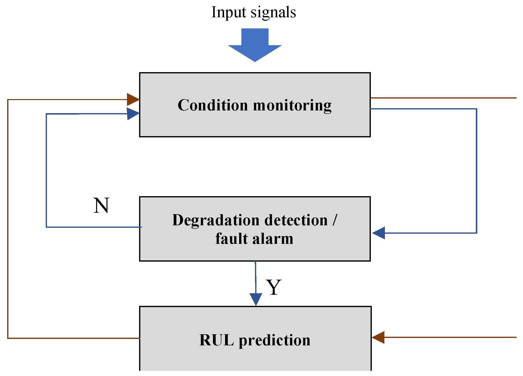
3. Problem Definition

The RUL of a WT gearbox bearing, also known as the first passage time (FPT), can be defined as the total remaining working duration (hours or revolutions) before a failure occurs, where the failure usually refers to the health status of the bearing when first hitting the pre-set failure threshold (FT) [8]. Generally, the full life cycle of a WT gearbox bearing contains the healthy running phase and the performance degradation phase, and the RUL prediction usually starts from the beginning of the performance degradation phase [18,32,33]. Hence, the RUL decreases linearly after the initial degradation is identified or there is a fault alarm of the monitoring system.

The relationship between condition monitoring and RUL prediction is depicted in Figure 2, where “Y” represents “yes”, and “N” represents “No”. The condition monitoring based on input signals of sensor data covers the whole lifetime of an equipment, aiming at detecting the initial performance degradation, namely, the time when the monitored measurements depart from the normal measurements, and sending out fault alarm signals [34]. Once an alarm is triggered, the task of RUL prediction starts. The trigger condition of RUL prediction is based on the existing monitoring system fault alarm in this work.

Let $\lambda$ represent the FT of the WT gearbox bearing. The RUL $L$ can be described using the formula:

$$L=inf\left\{l:x\left(l+t_k\right)\ge \lambda |x\left(t_k\right)<\lambda \right\}$$

(1)

where $inf\left\{·\right\}$ is the inferior limit of the value of $l$ that satisfies the constraints; $t_k$ is the current time; $x\left(·\right)$ is the health status of the bearing at the corresponding time. In addition, the expression is based on the condition that the health status of the current time $x\left(t_k\right)$ does not reach the FT $\lambda$.

It is worth mentioning that quite a few existing works [18,35,36,37] focus on predicting the RUL of a bearing whose sensor data have been used for model training. The nature of this is the equivalent use of a training set and testing set. However, only predicting the RUL of a bearing that has not failed and is unseen by the trained model is valuable in practice, as opposed to a historical one or one that has already failed. Therefore, we conduct the training phase of the proposed method using a small historical dataset, while the testing phase is based on other data. This problem challenges the generalization ability of the method.

4. The Proposed Method

The proposed method mainly involves five steps, as shown in Figure 3. The offline processes are represented by black arrows, and the online process is marked by a red arrow. The data or model access processes are marked by dotted arrows.

First, the Wiener degradation model is constructed and trained using the limited historical data covering the full degradation processes of several failed WT gearbox bearings. The standard training process of DNNs does not require manual rules. The additional rules or guidance introduced for training DNNs better are known as the prior knowledge. In this method, the independent incremental process assumption addressed by the Wiener model is the prior knowledge, which means that the degradation increments in different periods are independent and Gaussian. Although the assumption may not be always satisfied in practice, many works [9,38,39] have shown that it can yield acceptable results; moreover, the knowledge bias within a certain range is tolerable in this method.

Second, based on the trained Wiener model, the samples, including their RULs, are augmented based on the presented stochastic degradation path simulation method. The simulation process is expected to take full advantage of the Wiener process architecture and output the augmented data following the prior knowledge and the degradation trend of historical data.

Third, the novel DNN, namely, PI-LSTM, is constructed and trained using the augmented data with their RUL labels. In this step, the knowledge of the Wiener process model is fully absorbed in a data-driven way. In the PI-LSTM, the relation descriptions between the performance data and their RULs are no longer based on any explicit formulas or certain knowledge but rather on stacked neurons and weights. From a point of view, the degradation laws are first torn apart and then rebuilt. The core value is that this can help to eliminate the knowledge bias via the information of raw data, with no human assumptions involved, which is the purpose of the PI-LSTM fine-tuning process using the original historical data in step 4.

The previous steps comprise the offline phase of the whole method. Finally, the fine-tuned PI-LSTM is used for the online RUL prediction of the WT gearbox bearings in service using newly collected performance data as inputs based on the forward propagation process.

4.1. Wiener Degradation Model Construction and Training

The Wiener process is the mathematical model of Brownian motion, which refers to the irregular motion of particles suspended in liquid or gas when they collide. The displacement of the particle in the time period $\left(s,t\right)$can be regarded as the sum of multiple decomposition displacements. Assuming that the displacement $W\left(t\right)-W\left(s\right)$ follows a normal distribution according to the central limit theorem, the directions and magnitudes of the impulsive forces on particles in non-overlapping time periods can be considered to be independent of each other; thus, the displacement $W\left(t\right)$ has an independent increment. Based on this, the probability distribution of particle displacement in a certain period of time is only related to the time interval length and is unrelated to the initial moment.

4.1.1. The Construction of the Wiener Model

Considering the uncertainty of the performance degradation process of the WT gearbox bearing, a general Wiener model based on the state [40] is used to describe this process after the fault alarm of the system. $x\left(t\right)$ is used to represent the health status of the bearing on time point $t$, which can be calculated by feature extraction and fusion based on the sensor data related to the bearing. In this paper, we refer to the method in reference [41] for health status construction with high trendability and monotonicity. This method adopts an end-to-end DNN for automatically extracting the degradation-related features from the raw vibration signals of bearings after normalization, with no need for expert knowledge. Since the constructed health indicator (HI) in reference [41] decreases with degradation ranging from 0 to 1, the 1-HI is finally used as the health status for adapting to this paper. Let the initial time point $t=0$; then, the Wiener process model can be described as:

$$x\left(t\right)=x\left(0\right)+{{\displaystyle \int }}_0^t\mu \left(x\left(\tau \right)\right)d\tau +{{\displaystyle \int }}_0^t\sigma \left(\tau \right)dB\left(\tau \right)$$

(2)

where $\tau$ is the time term in the integral; $\mu \left(x\left(\tau \right)\right)$ represents the instantaneous degradation rate, which is a function of the health status $x\left(\tau \right)$; $\sigma \left(\tau \right)$ is the diffusion coefficient function describing the variance of random fluctuations that can be estimated by polynomial fitting; $B\left(\tau \right)$ describes the standard Brownian motion.

Based on Equation (2), the transition function of the health status of the WT gearbox bearing can be derived by:

$$x\left(t_k\right)=x\left(t_{k-1}\right)+\mu \left(x\left(t_{k-1}\right),\mathit{\theta }\right)\Delta t_{k-1}+{\omega }_{k-1}$$

(3)

where $\mu \left(x\left(t_{k-1}\right),\mathit{\theta }\right)$ represents the instantaneous degradation rate at time $t_{k-1}$ and $\mathit{\theta }$ is the unknown parameters in the function. The form of $\mu \left(·\right)$ can be determined by the Akaike information criterion (AIC) or the Bayesian information criterion (BIC), and $aexp\left(bx\left(t_{k-1}\right)\right)$ is selected based on AIC. $\Delta t_{k-1}=t_k-t_{k-1}$ is the time interval; ${\omega }_{k-1}\sim N\left(0,{\sigma }^2\left(t_{k-1},\mathit{\epsilon }\right)\Delta t_{k-1}\right)$ is the error term; $\mathit{\epsilon }$ is the unknown parameter. $\mathit{\theta }$ and $\mathit{\epsilon }$ in the transition function will be estimated through the offline training process.

4.1.2. The Offline Training of the Constructed Wiener Model

To obtain the unknown parameters $\mathit{\theta }$ and $\mathit{\epsilon }$ in the transition function, the limited historical data of failed bearings are used to conduct the parameter estimation. Due to the few unknown parameters, the demand for the amount of training data is relatively low. Based on this, the basic laws of the degradation process of WT gearbox bearings in the Wiener framework can be derived.

Assuming that there are N groups of time-series historical health status samples $X={\left\{{\mathit{X}}^n\right\}}_{n=1:N}$, with each group of samples, ${\mathit{X}}^n$ comes from the whole degradation process of an individual (the nth) bearing of the WT gearbox, starting with the fault alarm and ending with its failure. The nth group of samples can be represented by ${\mathit{X}}^n={\left(x_{n,1},x_{n,2},\dots ,x_{n,K_n}\right)}^{\mathrm{T}}$, where $x_{n,K_n}$ is the health status of the nth bearing on the $K_n$th time point. This expression is slightly different from $x\left(t\right)$, when we introduce the general form of the transition function in Section 4.1.1 based on the specific time point $t$, since it is more applicable to the sampling method of current SCADA sensors at regular intervals using the serial number $K_n$. Hence, $x_{n,k}$ is equivalent to $x_n\left(t_k\right)$.

Based on Equation (3), $\Delta x_{n,k-1}=x_{n,k}-x_{n,k-1}=\mu \left(x_{n,k-1},\mathit{\theta }\right)\Delta t_{k-1}+{\omega }_{k-1}$ follows the distribution $N\left(\mu \left(x_{n,k-1},\mathit{\theta }\right)\Delta t_{n,k-1},{\sigma }^2\left(t_{n,k-1},\mathit{\epsilon }\right)\Delta t_{n,k-1}\right)$. Therefore, the log-likelihood function of the unknown parameters $\mathit{\theta }$ and $\mathit{\epsilon }$ can be obtained:

$$\begin{array}{cc}ℒ\left(\mathit{\theta },\mathit{\epsilon }|X\right)=-{\displaystyle {\displaystyle \sum }_{n=1}^N}\hfill & \frac{K_n-1}{2}\ln \left(2\pi \right)\hfill \\ & -{\displaystyle {\displaystyle \sum }_{n=1}^N}{\displaystyle {\displaystyle \sum }_{k=1}^{K_n-1}}(\frac{1}{2}\ln \left({\sigma }^2\left(t_{n,k-1},\mathit{\epsilon }\right)\Delta t_{n,k-1}\right)\hfill \\ & +\frac{{\left(\Delta x_{n,k-1}-\mu \left(x_{n,k-1},\mathit{\theta }\right)\Delta t_{n,k-1}\right)}^2}{2{\sigma }^2\left(t_{n,k-1},\mathit{\epsilon }\right)\Delta t_{n,k-1}})\hfill \end{array}$$

(4)

The final estimated values of $\mathit{\theta }$ and $\mathit{\epsilon }$, represented by $\tilde{\mathit{\theta }}$ and $\tilde{\mathit{\epsilon }}$, can be calculated by maximizing Equation (4). In addition, the transition function is also obtained by substituting the estimated values of $\mathit{\theta }$ and $\mathit{\epsilon }$ into Equation (3).

4.2. Wiener Degradation Model Construction and Training

The Wiener process model obtained by offline training based on a small amount of historical data can represent the basic law of the performance degradation process of WT gearbox bearings. To further expand the law, it is necessary to simulate a large number of degradation trajectories of different WT gearbox bearings. Their RULs are calculated for data augmentation, namely, expanding the dataset based on rules and formulas, which is a common method for avoiding overfitting and increasing generalizability. Due to the stochastic variables in Equation (3), there are theoretically countless possible degradation trajectories. With the help of the transition function of Equation (3), the stochastic degradation trajectories simulation method is proposed, as shown in Figure 4.

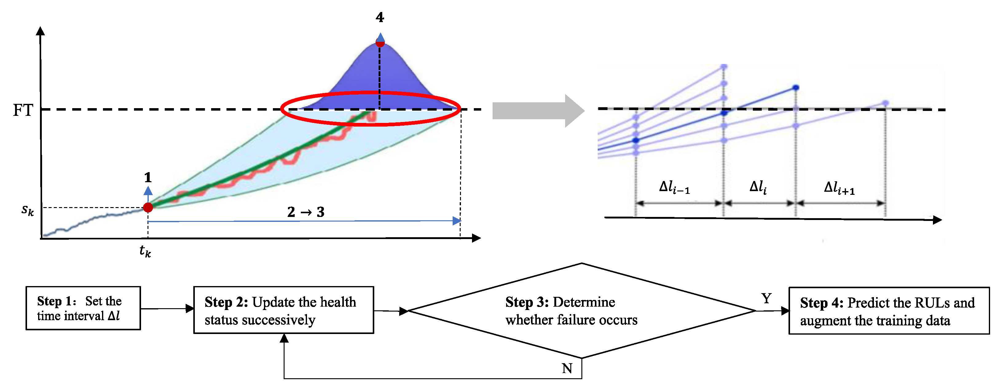
• Set the time interval of the health status transition $\Delta l$. Normally, if high-frequent signals are collected, the time interval can be set to a multiple of the data acquisition interval of sensors. Otherwise, $\Delta l$ can be equivalent to the data acquisition interval. In addition, a total of $N^{\prime }$ particles ${\left\{s_n\left(t_k\right)=s_{n, k}\right\}}_{n=1:N^{\prime }, k=1:K_n}$ are generated, representing $N^{\prime }$ virtual WT gearbox bearings, where $s_{n, k}$ is the initial health status of the nth bearing.
• Update the health status successively based on the transition function derived by Equation (3):

  $$s_n\left(l_i+t_k\right)=s_n\left(l_{i-1}+t_k\right)+\mu \left(s_n\left(l_{i-1}+t_k\right),l_{i-1}+t_k|\tilde{\mathit{\theta }}\right)\Delta l+{{\omega }_{i-1}|}_{\tilde{\mathit{\epsilon }}}$$

  (5)

  where $s_n\left(l_i+t_k\right)$ is the health status of the nth particle after the ith transition interval, $i=\left\{2, 3, 4, \dots \right\}$; $l_i=i\Delta l$.
• In the ith transition interval $\Delta l=l_i-l_{i-1}$, determine whether each particle fails according to the relationship between the health status $s_n\left(l_i+t_k\right)$ and the FT $\lambda$. If the particles have not failed, repeat step 2 until the health statuses of all particles reach or exceed $\lambda$; then, go to step 4.
• The probability density function of the RUL of the nth particle at $s_{n,k}$ can be estimated based on the analytical solution derived by sending the health status $s_{n,k}$ to the discrete probability density function of the RUL in the Wiener process [40,42]:

  $$\begin{array}{c}f\left(l|s_{n,k}\right)\cong \left(\frac{\lambda -s_{n,k}-{{\displaystyle \int }}_0^l\mu \left(s_n\left(\tau +t_k\right)\right)d\tau }{{{\displaystyle \int }}_0^l{\sigma }^2\left(\tau +t_k\right)d\tau }+\frac{\mu \left(s_n\left(l+t_k\right),l+t_k\right)}{{\sigma }^2\left(l+t_k\right)}\right)\frac{{\sigma }^2\left(l+t_k\right)}{\sqrt{2\pi {{\displaystyle \int }}_0^l{\sigma }^2\left(\tau +t_k\right)d\tau }}\\ \times exp\left(-\frac{{\left(\lambda -s_{n,k}-{{\displaystyle \int }}_0^l\mu \left(s_n\left(\tau +t_k\right)\right)d\tau \right)}^2}{2{{\displaystyle \int }}_0^l{\sigma }^2\left(\tau +t_k\right)d\tau }\right)\end{array}$$

  (6)

The passing sequence of the health status $s_{n,k}$ of each degradation trajectory and the corresponding RUL represented by $l_{n,k}$ that is uniformly sampled from Equation (6) collectively constitute the augmented dataset ${\left\{s_{n,k},l_{n,k}\right\}}_{n=1:N^{\prime },k=1:K_n}$. It can be used for training PI-LSTM, which performs the online RUL prediction of the WT gearbox bearing.

4.3. PI-LSTM Construction and Training

The widely used LSTM, as well as its variants, have shown good performances in the RUL prediction of WT components by dealing with the problems of vanishing or exploding gradients and the long-term dependence of time-series data, as explained in Section 2.1. However, the main bottleneck lies in the fact that the current input and the previous hidden state are fed into the current memory cell independently of each other. This makes it difficult for the memory cell of LSTMs to directly interact with the two parts, especially when the times-series sensor data are interrupted or interfered. Based on this, the Pre-Interaction LSTM (PI-LSTM) is proposed for predicting the RUL of the WT gearbox bearing online.

4.3.1. The Construction of PI-LSTM

Motivated by Mogrifier LSTM [43], an idea to break through the bottleneck of the existing LSTMs is to pre-interact the current input ${\mathit{x}}^t$ and the previous hidden state ${\mathit{h}}^{t-1}$ before it is sent to the current memory cell, thus increasing the ability to represent the sequential features of sensor data. In PI-LSTM, this function is realized by two novel gate mechanisms, $G$ and $H$, as shown in Figure 5. Taking the first layer as an example, let ${\mathit{x}}_{new}^t$ and ${\mathit{h}}_{new}^t$ represent the input and hidden state at time point $t$ after going through the new gates. The computational formula can be described as follows:

$${\mathit{x}}_{new}^t=2\mathsf{\sigma }\left(G^t{\mathit{h}}^{t-1}\right){\displaystyle ⨀}{\mathit{x}}^t$$

(7)

$${\mathit{h}}_{new}^t=2\mathsf{\sigma }\left(H^t{\mathit{x}}^{t+1}\right){\displaystyle ⨀}{\mathit{h}}^t$$

(8)

where $G^t$ and $H^t$ are the introduced trainable interaction matrices, representing the interaction mode between the two parts; ⨀ is the elementwise product; $\sigma \left(·\right)$ is the Sigmoid activation function. The necessity of multiplying by two lies in the fact that it ensures that the $G^t$ and $H^t$ with random initialization form transformations close to the identity, since the average output value of Sigmoid is 0.5. It plays an important role in confining the magnitude of the transferring gradient and controlling the convergence speed of PI-LSTM.

It can be found that the final input ${\mathit{x}}_{new}^t$ fed into the memory cell at time point $t$ is obtained by the interaction between the previous hidden state ${\mathit{h}}^{t-1}$ and the original current input ${\mathit{x}}^t$ through $G^t$, and the final hidden state ${\mathit{h}}_{new}^t$ sent to the memory cell at time point $t+1$ is obtained by the interaction between the original next input ${\mathit{x}}^{t+1}$ and the original hidden state ${\mathit{h}}^t$ through $H^t$. Based on this mechanism, there is no possibility that the obtained new input and hidden state are independent of each other, which helps the memory cell to more easily capture the feature representations of sequential correlations.

Please note that there are mainly two differences between the proposed PI-LSTM and the Mogrifier LSTM [43]. Firstly, the Mogrifier LSTM only considers interaction using the past experiences, while the ${\mathit{h}}_{new}^t$ in PI-LSTM is calculated based on ${\mathit{x}}^{t+1}$ instead of ${\mathit{x}}^t$ in the Mogrifier LSTM. This is quite important, since it is only in this way that the ${\mathit{x}}^{t+1}$ and ${\mathit{h}}_{new}^t$ can interact before they meet in the memory cell. Secondly, in the Mogrifier LSTM, the inputs and hidden states are updated alternately, and this can prevent the interrupted information from being captured in the rapidly changing situations. Instead, the interaction matrices of PI-LSTM update together step by step.

In addition, PI-LSTM follows the original gates mechanism in the memory cells of LSTM (see Figure 6). Taking the first layer as an example, the iterative formulas in the time dimension can be summarized as follows:

$${\mathit{i}}^t=\sigma \left(W^i{\mathit{x}}_{new}^t+V^i{\mathit{h}}_{new}^{t-1}+{\mathit{b}}^i\right)$$

(9)

$${\mathit{f}}^t=\sigma \left(W^f{\mathit{x}}_{new}^t+V^f{\mathit{h}}_{new}^{t-1}+{\mathit{b}}^f\right){\mathit{h}}_{new}^t=2\mathsf{\sigma }\left(H^t{\mathit{x}}^{t+1}\right){\displaystyle ⨀}{\mathit{h}}^t$$

(10)

$${\mathit{o}}^t=\sigma \left(W^o{\mathit{x}}_{new}^t+V^o{\mathit{h}}_{new}^{t-1}+{\mathit{b}}^o\right)$$

(11)

$${\mathit{s}}^t={\mathit{f}}^t{\displaystyle ⨀}{\mathit{s}}^{t-1}+{\mathit{i}}^t{\displaystyle ⨀}\tan \mathrm{h}\left(W^s{\mathit{x}}_{new}^t+V^s{\mathit{h}}_{new}^{t-1}+{\mathit{b}}^s\right)$$

(12)

$${\mathit{h}}^t={\mathit{o}}^t{\displaystyle ⨀}\tan \mathrm{h}\left({\mathit{s}}^t\right)$$

(13)

where ${\mathit{i}}^t$, ${\mathit{f}}^t$, ${\mathit{s}}^t$ and ${\mathit{o}}^t$ represent the input gate, forget gate, state of cell and output value of the output gate at time point $t$, respectively; $W^{*}$ and $V^{*}$ are the weight matrices; ${\mathit{b}}^{*}$ is the corresponding bias. In summary, PI-LSTM is constructed and then trained offline based on the augmented data.

4.3.2. The Offline Training of the Constructed PI-LSTM

The offline training of the constructed PI-LSTM is mainly based on the back propagation algorithm using the augmented data ${\left\{s_{n,k},l_{n,k}\right\}}_{n=1:N^{\prime },k=1:K_n}$. The health status $s_{n,k}$ of each degradation trajectory and the corresponding RUL $l_{n,k}$ are fed into the PI-LSTM as the training inputs and labels, respectively. Please note that the augmented data do not include the original historical data. The main difference between them is that the data augmentation contains a knowledge bias, while the original data can directly reflect the real performance variations. Predicting the RUL of the WT gearbox bearing is a typical regression problem. The predicted value ${\tilde{l}}_{n,k}$ of PI-LSTM is expected to approximate the label value $l_{n,k}$ based on iteratively updating the parameters of PI-LSTM $\mathit{\theta }$ using the stochastic gradient descent (SGD) algorithm. The loss function is the mean square error (MSE) between the predicted values and the label values of the whole augmented data:

$$\underset{\mathit{\theta }}{\min }{{\displaystyle \sum }}_{n,k}{\Vert {\tilde{l}}_{n,k}-l_{n,k}\Vert }^2$$

(14)

In addition, the dropout technique is used to prevent overfitting. Generally, the dropouts for LSTMs can be divided into three categories, which exist between the input and the first hidden layer (the first type) inside each hidden layer (the second type) and across multiple hidden layers (the third type). Since the $G^t$ and $H^t$ are interconnected with the hidden state and the input, the matrix $G^t$ is skipped when the dropout between the input ${\mathit{x}}^t$ and the memory cell ${\mathit{h}}^t$ works, and the matrix $H^t$ is skipped when the dropout from the memory cell ${\mathit{h}}^t$ to ${\mathit{h}}^{t+1}$ inside the hidden layer works.

4.4. PI-LSTM Fine-Tuning

The offline-trained PI-LSTM characterizes the comprehensive feature variations of the performance degradation processes of WT gearbox bearings based on the augmented data with strong statistical significance. Considering the introduced bias of the Wiener model, the PI-LSTM further requires a correction process based on real data, which is the value of fine-tuning. Fine-tuning takes advantage of the pre-trained PI-LSTM containing the degradation regularity of the original historical data, based on which the mapping relationship from samples to RULs is adjusted at the least cost. The most popular way of fine-tuning is to first freeze the lower layers of DNNs and then update the parameters of the top layers based on the back propagation algorithm using the tuning dataset. However, it is not suitable for situations in which tuning data are limited, since the network is prone to overfitting. Hence, an additional polynomial fitting above the top layer of PI-LSTM is introduced, which is also an effective trick of fine-tuning DNNs.

Keeping the parameters of the offline-trained PI-LSTM unchanged, the N groups of time-series historical health status samples ${\left\{x_{n,k}\right\}}_{n=1:N, k=1:K_n}$ are sequentially processed by the stacked layers of PI-LSTM as inputs, and the predicted RUL results ${\left\{l_{n,k}^{\prime }\right\}}_{n=1:N, k=1:K_n}$ can be obtained. For these health status samples, the real RULs are given. Hence, by using ${\left\{l_{n,k}^{\prime }\right\}}_{n=1:N, k=1:K_n}$ as inputs and the RUL labels as outputs, the additional polynomial fitting is used for adjusting the predicted results to the real RULs.

4.5. RUL Prediction of WT Gearbox Bearings

The RUL prediction of WT gearbox bearings is based on the forward propagation of the fine-tuned PI-LSTM. The bearings to be predicted should not appear in the training phase in case of eavesdropping. Specifically, the real-time health status derived by sensor-collected data is fed into the PI-LSTM in practical use, and then the online RUL can be obtained. To fully test the method, the overall historical data and their corresponding RULs are used, and the evaluation metrics can be applied for quantitative comparison with the state-of-the-art. Please note that the testing data do not require complete records covering the overall degradation process of bearings, which further relieves the need for method testing. More details are illustrated in Section 5.

5. Case Study

In this section, the experimental setups and statistical results based on the real-world SCADA data of WT gearbox bearings are presented to show the effectiveness of the proposed method. First, the data collection details are provided. Second, the experimental details of parameter selection, hyper-parameter setting and other setups are explained. Finally, the key parts of the proposed method are validated, and the statistical results, as well as the visualizations, are shown and compared with several state-of-the-art methods.

5.1. Data Collection

The data used in this experiment have been collected from 3 May 2018 to 4 January 2022 at a wind farm located in Inner Mongolia, northern China. The dataset contains a total of 18 three-bladed modern WTs (shown in Figure 7) with 2 MW of nominal power. The WTs are equipped with gearboxes of identical configurations. The technical parameters of the WTs are illustrated in

Table 1. Technical parameters of the WTs.

Technical Parameter	Value
Rated power	2000 kW
Cut-in wind speed	5 m/s
Rated wind speed	13 m/s
Cut-out wind speed	24 m/s
Rotor diameter	90 m
Rotor-swept area	6476 m2
Number of blades	3
Maximum rotor speed	14.9 rpm
Tip speed	70 m/s
Maximum generator speed	2014 rpm
Generator voltage	700 V
Grid frequency	52 Hz
Hub height	76 m

. Two tapered roller bearings and a cylindrical roller bearing are installed in each gearbox, and the tapered roller bearing is the object of this study, named the high-speed shaft (HSS) bearing. Most HSS bearings encountered cracking failures according to the logs. The failed HSS bearing was replaced with a new one after the failure occurred.

The existing system is equipped with a fault alarm mechanism, which sends out the alarm signal once it detects the initial performance degradation of gearbox bearings. The recorded data and logs of SCADA contain 54-dimensional sensor-collected data related to the WTs, environmental data, fault alarm time, failure time and failure cause of each component or part of the WTs, as well as their replacement time. The sensor data of WTs consist of two types: behavioral parameters and performance parameters. The former refers to the data that describe the active behaviors of WTs under the default control strategies, and the latter refers to the parameters signifying the health conditions of the corresponding parts or components of WTs.

5.2. Experimental Details

5.2.1. Parameter Selection

The monitored parameters are first selected for the subsequent feature extraction and other processes. The sensor-collected data related to the HSS bearings are high-frequency vibration signals with a sampling frequency of 25 kHz which contain the degradation information of the monitored HSS bearing [44]. In addition, selecting the other monitored parameters indirectly related to the performance of the HSS bearing is also useful, since they provide observations of other perspectives, enriching the amount of input information.

By calculating the correlation coefficients, several monitored parameters that are statistically significantly related to the vibration signals of HSS bearings are further selected, including the environmental parameters wind speed and ambient temperature, the behavioral parameter rotor speed and the performance parameter active power. The low-frequency parameters are sampled with 2 min intervals, and their averaged measurements in each interval are given in the dataset. The samples of the selected SCADA parameters for a certain period are illustrated in Figure 8.

5.2.2. Hyper-Parameter Setting

The structural parameters for the health status construction method refer to the settings in reference [41], shown in

Table 2. Structural parameters of DNN for health status construction.

No.	Layer	[Kernel Size, Channel], Stride	Output Size
0	Input	/	$1\times L_n$
1	Conv_1	$\left[16,32\right],1$	$32\times L_n$
2	Residual_block_1	$\left[\begin{array}{c}16,32\\ 16,32\end{array}\right],1$	$32\times L_n$
3	Residual_block_2	$\left[\begin{array}{c}16,32\\ 16,32\end{array}\right],4$	$32\times L_n/4$
4	Residual_block_3	$\left[\begin{array}{c}16,64\\ 16,64\end{array}\right],2$	$64\times L_n/8$
5	Residual_block_4	$\left[\begin{array}{c}16,64\\ 16,64\end{array}\right],4$	$64\times L_n/32$
6	LSTM	/	$4\times L_n/32$
7	Fully connected	/	1

. The selected input samples of each dimension are used for health status construction individually. The constructed health statuses of the high-frequency vibration data at every 2 min are first averaged for interval alignment with the low-frequency parameters. Then, the health statuses of the data for different dimensions in the same periods are averaged for calculating the final health status in units of 2 min. The time interval of health status transition ∆l is set to 2 min.

The hyper-parameters of the presented method are determined based on the tuner using batched Gaussian Process Bandits [45]. The highest power of polynomial fitting of $\sigma \left(\tau \right)$ determines the fitting ability of the Wiener process model. When it is set as 4, the model is able to include sufficient information of prior knowledge for the subsequent stochastic degradation trajectories simulation while avoiding overfitting. The learning rate and its decay rate of PI-LSTM also play key roles in model training. A higher learning rate makes the model update faster but harder to converge, while a lower learning rate increases the training time. Hence, the learning rate is set in a gradually decaying form as the number of iterations increases. It helps the PI-LSTM update fast at the beginning of training and then gradually slow down, converging finally. When the learning rate equals 0.005 and the decay rate of the learning rate equals to 0.98, the PI-LSTM is able to converge to its optimum. The number of hidden layers of PI-LSTM determines the order of magnitude of training parameters. When it equals 3, the PI-LSTM shows the best fitting ability. The setting of the dropout rates of three types requires trial and error. The values of 0.2, 0.2 and 0.45 make the model training both smooth and optimal. The highest power of polynomial fitting on the top of PI-LSTM is important for fine-tuning the introduced prior knowledge based on the Wiener model and eliminating the bias of knowledge. When it is set as 3, the method achieves its highest accuracy. These optimized hyper-parameters are given in

Table 3. Hyper-parameters of the presented method.

Model	Hyper-Parameters	Value
Wiener degradation model	The highest power of polynomial fitting of $\sigma \left(\tau \right)$	4
PI-LSTM	Learning rate	0.005
	Decay rate of learning rate	0.98
	Number of hidden layers	3
	Dropout rate (the first type)	0.2
	Dropout rate (the second type)	0.2
	Dropout rate (the third type)	0.45
	The highest power of polynomial fitting on the top	3

.

The failure time of the HSS bearings according to the log can be used for determining the value of FT $\lambda$. The health status of each historical bearing on the failure time is first calculated. It can be found that the range of the obtained final health statuses is small, ranging from 0.846 to 0.863. Hence, we finally use the weighted average value of the final health statuses as the value of FT $\lambda$, which equals 0.858. The $\lambda$ is further used for the RUL labeling of the training data and augmented data, as well as for the RUL prediction of the HSS bearings in the testing phase.

5.2.3. Other Details

Besides the abovementioned experimental setups, other details are introduced in this part. The number of groups of time-series historical health status samples $N$ is 5, which is a quite small raw dataset for the RUL prediction task under complex operating conditions. These samples are used for the offline training of the Wiener model according to Section 4.1. A total of 96 degradation trajectories of virtual bearings are simulated for the offline training of PI-LSTM according to Section 4.2 and Section 4.3.

For testing the effect of the RUL prediction of the WT gearbox bearing, a five-fold cross-validation is applied. Specifically, the raw dataset is divided into five groups, and four of them are used as both the training data for the Wiener model and the data source for the simulation and polynomial fitting on top of the PI-LSTM, according to Section 4.4. One of them is used as testing data in order to predict the RULs and calculate the metrics. A total of three cross-validations are conducted for balancing the disturbance of random factors.

5.3. Results and Discussion

5.3.1. Metrics for RUL Prediction

Two metrics are used for quantitatively measuring the accuracy of predicting the RUL in hours. The first one is S-score [46], derived by:

$$S=\{\begin{array}{c}\begin{array}{cc}\frac{1}{{{\displaystyle \sum }}_{m=1}^M{T}_m}{\displaystyle \sum }_{m=1}^M{\displaystyle \sum }_{t=1}^{T_m}\left(e^{-\frac{h_{m,t}}{13}}-1\right)& h_{m,t}<0\end{array}\\ \begin{array}{cc}\frac{1}{{{\displaystyle \sum }}_{m=1}^M{T}_m}{\displaystyle \sum }_{m=1}^M{\displaystyle \sum }_{t=1}^{T_m}\left(e^{\frac{h_{m,t}}{10}}-1\right)& h_{m,t}>0\end{array}\end{array}$$

(15)

where $h_{m,t}={\widetilde{RUL}}_{m,t}-RU{L}_{m,t}$ describes the deviation between the average predicted RUL of the mth group of historical data when used for testing on the tth sample ${\widetilde{RUL}}_{m,t}$ and the corresponding RUL label $RU{L}_{m,t}$; $T_m$ is the total number of samples in the mth group; $M$ is the total number of groups, which equals five in this experiment due to the five-fold cross-validation.

It can be found that the S-score gives different penalty weights for a prediction lag $h_{m,t}>0$ and a prediction advance $h_{m,t}<0$. If the prediction is ahead, an advance prediction can also help to repair or maintain before a failure occurs; hence, the penalty coefficient is lower. Otherwise, the penalty coefficient is higher, since a delay indicates an unexpected failure, which is more unacceptable.

The second metric is the root mean squared error (RMSE), which gives the same penalty weights for prediction lag and prediction advance, derived by:

$$\mathrm{RMSE}=\sqrt{\frac{1}{{{\displaystyle \sum }}_{m=1}^M{T}_m}{{\displaystyle \sum }}_{m=1}^M{{\displaystyle \sum }}_{t=1}^{T_m}{\left({\widetilde{RUL}}_{m,t}-RU{L}_{m,t}\right)}^2}$$

(16)

In summary, a higher S-score or RMSE means a larger prediction error. The S-score has more practice value, while the RMSE is widely used for measuring statistical results in theory.

5.3.2. Method Verification

To investigate the value of each part in the proposed method, an effect verification is necessary. Keeping the selected parameters and the health status construction method unchanged, several key parts of the proposed method are verified in this section. The calculated health status in the degradation process of one group of samples is illustrated in Figure 9. It can be found that the health status has good trendability and monotonicity. The verification is based on a variable-controlling approach by which experiments are conducted when replacing certain parts with a baseline method or directly removing the part. An effective part can yield more satisfiable results. When certain parts are replaced or removed, the hyper-parameters are re-optimized using the same techniques with Section 5.2.2 to show the best performances of the adjusted methods.

Specifically, we first verify the Wiener model and the simulation step as a whole, since, if the Wiener model is removed, the simulation part is pointless. Thus, the PI-LSTM is directly offline-trained to extract the features from the original health status samples, namely, the inputs of training, and the labels are the real RULs. Since no prior knowledge is involved, the PI-LSTM fine-tuning can also be omitted. In the testing phase, the RUL prediction is still based on the five-fold cross-validation, with $\lambda$ equaling 0.858, and the two metrics in the five groups of testing data are calculated.

Secondly, we investigate the effect of the novel DNN, PI-LSTM, by replacing it with several baseline DNNs including the standard LSTM, Bi-directional LSTM (Bi-LSTM) and Bi-LSTM with an attention mechanism (Bi-LSTM(A)) [47]. The number of hidden layers of each baseline method is three, which is the same as that with PI-LSTM. For the sake of fairness, the structures of the compared DNNs including PI-LSTM should be as identical as possible, while the values of hyper-parameters could be different. The testing phase is exactly the same as the process explained in Section 5.2.3.

Thirdly, we explore the effect of the PI-LSTM fine-tuning process, as explained in Section 4.4. On one hand, the fine-tuning is omitted; thus the offline trained PI-LSTM is directly used for the RUL prediction of HSS bearings. On the other hand, we adopt the widely used fine-tuning technique (frozen fine-tuning), which only updates the top layer of PI-LSTM using real historical samples, while the lower layers are frozen, instead of the polynomial fitting for comparison.

The statistical results of both metrics of the abovementioned conditions are shown in

Table 4. Statistical results of different conditions.

Method Condition	S-Score	RMSE
1. PI-LSTM only	2.53	1.46
2.$\mathrm{Wiener}\to$ LSTM $\to$ fine-tuning	2.88	1.83
3.$\mathrm{Wiener}\to$ Bi-LSTM $\to$ fine-tuning	2.63	1.70
4.$\mathrm{Wiener}\to$ Bi-LSTM(A) $\to$ fine-tuning	2.37	1.52
5.$\mathrm{Wiener}\to$ PI-LSTM	1.69	0.88
6.$\mathrm{Wiener}\to$ PI-LSTM$\to$ frozen fine-tuning	1.43	0.61
7.$\mathrm{Wiener}\to$ PI-LSTM$\to$ fine-tuning (the proposed method)	1.28	0.44

. The method condition with the best performances is highlighted, which is the complete process of the proposed method. It can be found that the two metrics show similar performance measurements. Based on the results, we can summarize a few points as follows.

• Each part of the proposed method has a good effect.

Through the comprehensive investigation, the effects of the key parts, including the introduced prior knowledge based on the Wiener process model and the degradation simulation, PI-LSTM and the fine-tuning step, have been verified. Quantitative analysis can be performed based on two metrics. For example, from the results of conditions 2, 3, 4 and 7, it can be found that the PI-LSTM shows stronger performances compared to the standard LSTM, the Bi-LSTM and the Bi-LSTM(A) with the same basic network structures, which yield a 1.60-, 1.35- and 1.09-higher S-score, respectively, and a 1.39-, 1.26- and 1.08-higher RMSE, respectively. This indicates the pre-interaction mechanism in PI-LSTM. The only variable part in the comparative conditions plays a very important role in this task. Similarly, the other parts also show their positive effects.

2.

The introduced prior knowledge shows a promising effect.

In the proposed method, the prior knowledge of the independent incremental process addressed by the Wiener model is introduced. Through the simulation process and data augmentation, the whole method learns from it and finally benefits from this. From Table 4, the result of condition 7 provides a 1.25-lower S-score and a 1.02-lower RMSE compared to the result of condition 1. Condition 1 directly uses the PI-LSTM to extract features from the raw limited samples, which could easily lead to overfitting. This is because trivial features of the samples are learned by PI-LSTM—even the contained noises.

3.

The deviations contained in the prior knowledge are reduced through fine-tuning.

From the results of conditions 5, 6 and 7, it can be found that the presented fine-tuning method successfully reduces the knowledge bias, lowering both the S-score and RMSE. The biased PI-LSTM that learned from the Wiener model is finally eliminated through the top polynomial fitting, which proves to be more effective than the frozen fine-tuning method, which easily overfits in situations of limited tuning data. In addition, the gap between the knowledge bias and the real conditions can be roughly measured by the 0.41 S-score and 0.44 RMSE differences between conditions 5 and 7. Since the final PI-LSTM in the proposed method may not perfectly fit the real performance degradation process of the HSS bearings, the gap can be even larger. In spite of this, the idea of using prior knowledge for data augmentation, followed by fine-tuning for bias elimination, still pays off, which is stimulating and promising.

5.3.3. Method Comparison

To demonstrate the performance of the complete method, the RUL prediction results on the same small dataset are horizontally compared with several state-of-the-art results, including the Moth Flame Optimization-based GRU (MGRU) [23], the multi-head neural network (MHNN) [14] and the multi-phase Wiener process model [8]. All works presented improved methods based on the well-known DNNs or empirical models in recent years, making them more competitive than the standard ones. The methods are performed using the same input features or health status samples as the input and following the same set-ups, such as the FT and the start time of the RUL prediction. In addition, the hy-per-parameters of the state-of-art, including the structure parameters such as the number of layers of the DNNs, are initialized according to the given values in each work and then tuned using the same tool [45] with our method.

Based on the same training set and cross-validation strategy, the average results of the methods can be obtained, as shown in

Table 5. Statistical results of different methods.

Method Condition	S-Score	RMSE
MGRU	3.23	1.72
MHNN	1.84	1.16
The multi-phase Wiener process model	2.06	1.27
The proposed method	1.28	0.44

. According to the statistical results, it can be seen that the proposed method achieves the highest accuracy in terms of both S-score and RMSE. This indicates that the proposed method is more applicable to the rapidly changing operating conditions of wind turbines, as well as RUL prediction tasks with limited samples.

Taking one testing case from the samples as an example, the predicted RUL results of the state-of-art methods and our proposed method, as well as the real RUL, are illustrated in Figure 10. From the results, it can be seen that our proposed method obviously shows its superiority over the state-of-art methods in terms of the accuracy of the RUL prediction task due to its introduced prior knowledge and the novel PI-LSTM.

6. Conclusions

In this paper, a novel hybrid method, namely, the data-driven PI-LSTM supported by the prior knowledge of the Wiener process model, is proposed for the RUL prediction of WT gearbox HSS bearings with limited samples. The presented idea is innovative and meaningful in combining the advantages of both model-based methods or empirical models and the DL approaches. It also overcomes the drawbacks of both categories. In addition, the proposed method is also easy to extend by replacing the Wiener process model, PI-LSTM or other parts with other methods. Hence, it provides a new perspective for enhancing the performance of the current methods in this area. A series of experiments using limited samples have proved that the proposed method is able to effectively capture the sequential features of the performance degradation process of gearbox bearings. In addition, the necessity of each key part of the proposed method has also been verified.

The DL approaches have experienced fast development in the last 10 years, fully automating the abstract feature extraction from raw data. The combination of the end-to-end DL methods and valuable human knowledge can provide many insights for the RUL prediction tasks; however, very few studies have been presented. There is a possibility that introducing prior knowledge more related to the task can produce better effects, which we think is a potential development trend in the future.

References

1. Yucesan, Y.A.; Dourado, A.; Viana, F. A survey of modeling for prognosis and health management of industrial equipment. Adv. Eng. Inform. 2021, 50, 101404. [Google Scholar] [CrossRef]
2. Rezamand, M.; Kordestani, M.; Carriveau, R.; Ting, S.K.; Saif, M. Critical wind turbine components prognostics: A comprehensive review. IEEE Trans. Instrum. Meas. 2020, 69, 9306–9328. [Google Scholar] [CrossRef]
3. Breteler, D.; Kaidis, C.; Tinga, T.; Loendersloot, R. Physics based methodology for wind turbine failure detection, diagnostics & prognostics. In Proceedings of the European Wind Energy Association Annual Conference and Exhibition, Paris, France, 17–20 November 2015; pp. 1–9. [Google Scholar]
4. Li, Y.; Kurfess, T.; Liang, S.Y. Stochastic prognostics for rolling element bearings. Mech. Syst. Signal Process. 2000, 14, 747–762. [Google Scholar] [CrossRef]
5. Oppenheimer, C.H.; Loparo, K.A. Physically based diagnosis and prognosis of cracked rotor shafts. In Proceedings of the SPIE-The International Society for Optical Engineering, Orlando, FL, USA, 16 July 2002; Volume 4733, pp. 122–132. [Google Scholar]
6. Marble, S.; Morton, B.P. Predicting the remaining life of propulsion system bearings. In Proceedings of the IEEE Aerospace Conference, Big Sky, MT, USA, 4–11 March 2006. [Google Scholar]
7. Qiu, J.; Seth, B.B.; Liang, S.Y.; Zhang, C. Damage mechanics approach for bearing lifetime prognostics. Mech. Syst. Signal Process. 2002, 16, 817–829. [Google Scholar] [CrossRef]
8. Liao, G.B.; Yin, H.P.; Chen, M.; Lin, Z. Remaining useful life prediction for multi-phase deteriorating process based on Wiener process. Reliab. Eng. Syst. Safe. 2021, 207, 107361. [Google Scholar] [CrossRef]
9. Zhang, Z.X.; Si, X.S.; Hu, C.H.; Lei, Y.G. Degradation data analysis and remaining useful life estimation: A review on Wiener-process-based methods. Eur. J. Oper. Res. 2018, 271, 775–796. [Google Scholar] [CrossRef]
10. Zhang, C.; Kong, F.T. Application of gamma process and maintenance cost for fatigue damage of wind turbine blade. Energy Procedia 2019, 158, 3729–3734. [Google Scholar] [CrossRef]
11. Wang, J.J.; Liang, Y.Y.; Zheng, Y.H.; Gao, R.X.; Zhang, F.L. An integrated fault diagnosis and prognosis approach for predictive maintenance of wind turbine bearing with limited samples. Renew. Energy 2020, 145, 642–650. [Google Scholar] [CrossRef]
12. Merainani, B.; Laddada, S.; Bechhoefer, E.; Mohamed, A.A.C.; Benazzouza, D. An integrated methodology for estimating the remaining useful life of high-speed wind turbine shaft bearings with limited samples. Renew. Energy 2021, 182, 1141–1151. [Google Scholar] [CrossRef]
13. Jiang, J.R.; Lee, J.E.; Zeng, Y.M. Time series multiple channel convolutional neural network with attention-based long short-term memory for predicting bearing remaining useful life. Sensors 2020, 20, 166. [Google Scholar] [CrossRef] [Green Version]
14. Liu, Z.Y.; Liu, H.; Jia, W.J.; Zhang, D.H.; Tan, J.R. A multi-head neural network with unsymmetrical constraints for remaining useful life prediction. Adv. Eng. Inform. 2021, 50, 101396. [Google Scholar] [CrossRef]
15. Cheng, Y.W.; Hu, K.; Wu, J.; Zhu, H.P.; Shao, X.Y. A convolutional neural network based degradation indicator construction and health prognosis using bidirectional long short-term memory network for rolling bearings. Adv. Eng. Inform. 2021, 48, 101247. [Google Scholar] [CrossRef]
16. Desai, A.; Guo, Y.; Sheng, S.; Phillips, C.; Williams, L. Prognosis of wind turbine gearbox bearing failures using SCADA and modeled data. In Proceedings of the Annual Conference of the Prognostics and Health Management Society, online, 9–13 November 2020. [Google Scholar]
17. Teng, W.; Zhang, X.L.; Liu, Y.B.; Kusiak, A.; Ma, Z.Y. Prognosis of the remaining useful life of bearings in a wind turbine gearbox. Energies 2016, 10, 32. [Google Scholar] [CrossRef]
18. Elasha, F.; Shanbr, S.; Li, X.C.; David, M. Prognosis of a wind turbine gearbox bearing using supervised machine learning. Sensors 2019, 19, 3092. [Google Scholar] [CrossRef] [PubMed]
19. Zhao, Z.B.; Wu, J.Y.; Wong, D.; Sun, C.; Yan, R.Q. Probabilistic remaining useful life prediction based on deep convolutional neural network. In Proceedings of the 9th International Conference on Through-life Engineering Services, Cranfield, Bedfordshire, UK, 3–4 November 2020. [Google Scholar]
20. Jia, X.J.; Han, Y.; Li, Y.J.; Sang, Y.C.; Zhang, G.L. Condition monitoring and performance forecasting of wind turbines based on denoising autoencoder and novel convolutional neural networks. Energy Rep. 2021, 7, 6354–6365. [Google Scholar]
21. Pan, Y.B.; Hong, R.J.; Chen, J.; Wu, W.W. A hybrid DBN-SOM-PF-based prognostic approach of remaining useful life for wind turbine gearbox. Renew. Energy 2020, 152, 138–154. [Google Scholar] [CrossRef]
22. Guo, L.; Li, N.P.; Jia, F.; Lei, Y.G.; Lin, J. A recurrent neural network based health indicator for remaining useful life prediction of bearings. Neurocomputing 2017, 240, 98–109. [Google Scholar] [CrossRef]
23. Wang, S.S.; Chen, J.; Wang, H.; Zhang, D.Z. Degradation evaluation of slewing bearing using HMM and improved GRU. Measurement 2019, 146, 385–395. [Google Scholar] [CrossRef]
24. Zhu, L.P.; Zhang, X.R. Time series data-driven online prognosis of wind turbine faults in presence of SCADA data loss. IEEE Trans. Sustain. Energy 2020, 12, 1289–1300. [Google Scholar] [CrossRef]
25. Sayah, M.; Guebli, D.; Noureddine, Z.; Masry, Z.A. Deep LSTM enhancement for RUL prediction using Gaussian mixture models. Automat. Control Comput. Sci. 2021, 55, 15–25. [Google Scholar] [CrossRef]
26. Wang, Y.Q.; Yao, Q.M.; Kwok, J.T.; Ni, L.M. Generalizing from a few examples: A survey on few-shot learning. ACM Comput. Surv. 2020, 53, 1–34. [Google Scholar] [CrossRef]
27. Li, F.F.; Fergus, R.; Perona, P. One-shot learning of object categories. IEEE Trans. Pattern Anal. Mach. Intell. 2006, 28, 594–611. [Google Scholar]
28. Vinyals, O.; Blundell, C.; Lillicrap, T.; Kavukcuoglu, K.; Wierstra, D. Matching networks for one shot learning. In Proceedings of the 30th Conference on Neural Information Processing Systems, Barcelona, Spain, 5–10 December 2016; pp. 3637–3645. [Google Scholar]
29. Yu, M.; Guo, X.X.; Yi, J.F.; Chang, S.Y.; Potdar, S.; Cheng, Y.; Tesauro, G.; Wang, H.Y.; Zhou, B. Diverse few-shot text classification with multiple metrics. In Proceedings of the Conference of the North American Chapter of the Association for Computational Linguistics: Human Language Technologies, New Orleans, LA, USA, 1–6 June 2018. [Google Scholar]
30. Vartak, M.; Thiagarajan, A.; Miranda, C.; Bratman, J.; Larochelle, H. A meta-learning perspective on cold-start recommendations for items. In Proceedings of the 31st International Conference on Neural Information Processing Systems, Los Angeles, CA, USA, 4–9 December 2017; pp. 6907–6917. [Google Scholar]
31. Chen, W.B.; Chen, W.Z.; Liu, H.X.; Wang, Y.Q.; Bi, C.L.; Gu, Y. A RUL prediction method of small sample equipment based on DCNN-BiLSTM and domain adaptation. Mathematics 2022, 10, 1022. [Google Scholar] [CrossRef]
32. Zhang, B.; Zhang, S.H.; Li, W.H. Bearing performance degradation assessment using long short-term memory recurrent network. Comput. Ind. 2019, 106, 14–29. [Google Scholar] [CrossRef]
33. Kong, Z.M.; Cui, Y.; Xia, Z.; Lv, H. Convolution and long short-term memory hybrid deep neural networks for remaining useful life prognostics. Appl. Sci. 2019, 9, 4156. [Google Scholar] [CrossRef]
34. Gao, Z.W.; Liu, X.X. An overview on fault diagnosis, prognosis and resilient control for wind turbine systems. Processes 2021, 9, 300. [Google Scholar] [CrossRef]
35. Kramti, S.E.; Saidi, L.; Ali, J.B.; Sayadi, M. Particle filter based approach for wind turbine high-speed shaft bearing health prognosis. In Proceedings of the 2019 IEEE International Conference on Signal, Control and Communication, Hammamet, Tunisia, 16–18 December 2019. [Google Scholar]
36. Teng, W.; Han, C.; Hu, Y.K.; Cheng, X.; Song, L.; Liu, Y.B. A robust model-based approach for bearing remaining useful life prognosis in wind turbines. IEEE Access 2020, 8, 47133–47143. [Google Scholar] [CrossRef]
37. Noman, K.; He, Q.; Peng, Z.K.; Wang, D. Dynamic degradation quantification of wind turbine high speed shaft bearing based on oscillation based sparsity indices. J. Phys. Conf. Ser. 2021, 1880, 012013. [Google Scholar] [CrossRef]
38. Hu, Y.G.; Li, H.; Shi, P.P.; Chai, Z.S.; Wang, K.; Xie, X.J.; Chen, Z. A prediction method for the real-time remaining useful life of wind turbine bearings based on the Wiener process. Renew. Energy 2018, 127, 452–460. [Google Scholar] [CrossRef]
39. Mu, S.; Su, Y.L.; Jing, K.; Li, C. Remaining life prediction of wind turbine bearing based on Wiener process. Mater. Sci. Eng. 2020, 788, 012089. [Google Scholar]
40. Li, N.P.; Lei, Y.G.; Guo, L.; Yan, T.; Lin, J. Remaining useful life prediction based on a general expression of stochastic process models. IEEE Trans. Ind. Electron. 2017, 64, 5709–5718. [Google Scholar] [CrossRef]
41. Chen, L.T.; Xu, G.H.; Zhang, S.C.; Yan, W.Q.; Wu, Q.Q. Health indicator construction of machinery based on end-to-end trainable convolution recurrent neural networks. J. Manuf. Syst. 2020, 54, 1–11. [Google Scholar] [CrossRef]
42. Lee, S.; Park, W.; Jung, S. Fault detection of aircraft system with random forest algorithm and similarity measure. Sci. World J. 2014, 6, 727359. [Google Scholar] [CrossRef] [PubMed] [Green Version]
43. Melis, G.; Kočiský, T.; Blunsom, P. Mogrifier LSTM. In Proceedings of the International Conference on Learning Representations, online, 26–30 April 2020. [Google Scholar]
44. Xiao, X.C.; Liu, J.X.; Liu, D.S.; Tang, Y.F.; Zhang, F. Condition monitoring of wind turbine main bearing based on multivariate time series forecasting. Energies 2022, 15, 1951. [Google Scholar] [CrossRef]
45. Golovin, D.; Solnik, B.; Moitra, S.; Kochanski, G.; Karro, J.; Sculley, D. Google vizier: A service for black-box optimization. In Proceedings of the 23rd ACM SIGKDD International Conference on Knowledge Discovery and Data Mining, Halifax, NS, Canada, 13–17 August 2017; pp. 1487–1495. [Google Scholar]
46. Chen, Z.; Wu, M.; Zhao, R.; Guretno, F.; Li, X. Machine remaining useful life prediction via an attention based deep learning approach. IEEE Trans. Ind. Electron. 2020, 68, 2521–2531. [Google Scholar] [CrossRef]
47. Rathore, M.S.; Harsha, S.P. Prognostics analysis of rolling bearing based on Bi-directional LSTM and attention mechanism. J. Fail. Anal. Prev. 2022, 22, 704–723. [Google Scholar] [CrossRef]
Figure 1. Diagrams for different FSL types.
Sustainability 14 12094 g001
Figure 2. Relationship of condition monitoring and RUL prediction.
Sustainability 14 12094 g002
Figure 3. Diagram of the proposed method.
Sustainability 14 12094 g003
Figure 4. Process of the stochastic degradation trajectories simulation.
Sustainability 14 12094 g004
Figure 5. Architecture of the PI-LSTM.
Sustainability 14 12094 g005
Figure 6. Schematic of a memory cell.
Sustainability 14 12094 g006
Figure 7. The structure of WT.
Sustainability 14 12094 g007
Figure 8. Illustration of samples of the selected SCADA parameters.
Sustainability 14 12094 g008
Figure 9. Illustration of the calculated health status of a group of samples.
Sustainability 14 12094 g009
Figure 10. Method comparison.
Sustainability 14 12094 g010