Article

Adaptive Intelligent Model Predictive Control for Microgrid Load Frequency

1
School of Electrical and Electronic Engineering, North China Electric Power University, Beijing 102206, China
2
Multidisciplinary Center for Infrastructure Engineering, Shenyang University of Technology, Shenyang 110870, China
3
Faculty of Civil Engineering, Technische Universität Dresden, 01067 Dresden, Germany
4
John von Neumann Faculty of Informatics, Obuda University, 1034 Budapest, Hungary
5
Institute of Information Engineering, Automation and Mathematics, Slovak University of Technology in Bratislava, 81237 Bratislava, Slovakia
*
Authors to whom correspondence should be addressed.
Sustainability 2022, 14(18), 11772; https://doi.org/10.3390/su141811772
Submission received: 29 July 2022 / Revised: 10 September 2022 / Accepted: 11 September 2022 / Published: 19 September 2022
(This article belongs to the Special Issue Artificial Intelligence and Sustainability)

Abstract

:
In this paper, self-tuning model predictive control (MPC) based on a type-2 fuzzy system for microgrid frequency is presented. The type-2 fuzzy system calculates the parameters and coefficients of the control system online. In the microgrid examined, there are sources of photovoltaic power generation, wind, diesel, fuel cells (with a hydrogen electrolyzer), batteries and flywheels. In simulating the load changes, changes in the production capacity of solar and wind resources as well as changes (uncertainty) in all parameters of the microgrid are considered. The performances of three control systems including traditional MPC, self-tuning MPC based on a type-1 fuzzy system and self-tuning MPC based on a type-2 fuzzy system are compared. The results show that type-2 fuzzy MPC has the best performance, followed by type-1 fuzzy MPC, with a slight difference between the two results.

1. Introduction

With the increasing consumption of electricity around the world, the electricity industry is facing issues such as the high cost of building new power plants and developing transmission networks, over-distribution and distribution, and environmental concerns. In order to overcome these problems, the reliability of customer service should be increased, congestion and losses in transmission and distribution lines should be reduced, and new and suitable renewable energy sources that have been introduced over the last two decades should be distributed. The benefits of renewable energy sources have led to plans to make more use of them in the electricity industry and to expand microgrids in most countries [1,2,3,4]. Microgrids, which consist of the interconnection of distributed production units and loads, are units that can work in two ways: connected to the grid or islanded. These units have many applications for supplying power to sensitive centers [5]. The main network issues are frequency and power fluctuations, which have received considerable attention both at intervals corresponding to operation and management (which aim to dampen power fluctuations) and at intervals corresponding to frequency control (LFC) [6]. In the case of frequency control, the goal is to quickly dampen fluctuations and to ensure the dynamic performance of the system, so that the fluctuations are in a satisfactory range. Numerous studies have been performed on frequency control in microgrids [7,8,9,10]. The research conducted for controller design has two main categories. The first category is controllers based on conventional methods, and the second category, which has made great progress in recent years, is controllers based on computational intelligence [11,12,13]. Controllers based on proportional-integral control (PI) and proportional-integral-reflective controllers (PID) based on coefficients determined by the Ziegler–Nichols method [14] and fractional order are used to control the frequency of drops in data [15]. One of the methods used to control the load frequency is the robust control method [16,17], H-Infinite Control (H) [18]. In [19,20], some methods have been presented based on the evolutionary algorithm and the iteration method.
The droop control methods (linear droop-based control [21] and non-linear droop-based control [22]) for microgrid frequency control is presented. In [23], To control the microgrid frequency, a sliding mode controller is presented. This controller is observer based. Many researchers used self-tuning PID controllers based on evolutionary algorithms, such as genetic algorithms (GA) or particle swarm optimization (PSO) [24], social spider optimization (SSO) [25] and biogeography-based optimization (BBO) [26] for frequency control in the microgrid. In [27,28,29,30], a fuzzy controller in which the coefficients have been determined using PSO [31], type-2 fuzzy logic [32] and GA-fuzzy [33] has been used for frequency control. Some researchers have also used secondary frequency control over the converter of renewable energy production sources to control the frequency [34]. One of the control methods that has been successful in all engineering fields is model predictive control (MPC) [35,36]. This control method is based on predicting the system behavior (from the mathematical model of the system) and generating a control signal to minimize the error. This controller has been used extensively to control the microgrid frequency. In all these articles, the sensitivity of the method to the accuracy of the system model is clear. In other words, in most of the mentioned research studies, it has been assumed that the changes in parameters and system behavior are small and limited. In the present paper, a self-tuning MPC for microgrid frequency control in the presence of a large uncertainty is presented. This article can be considered as a more advanced version of [37]. The differences between our work and the method in [37] are as follows:
  • In [37], a rule-based (lookup table) type-1 fuzzy method has been used, but we use a type-2 fuzzy method with a learning capability (based on training data).
  • In [37], only one parameter (control signal weighting coefficient) is estimated (by the fuzzy system), but in our article, the control signal weighting coefficient, the error (between the reference and predicted output) weighting coefficient, the predictor window length, the control window length, the battery source control gain and the flywheel source control gain are estimated and regularly updated.
  • The number of power resources in [37] is five cases and the flywheel is not considered, but we consider the flywheel power source to make our work comprehensive.
The control signal is applied to the renewable resources in the microgrid. Additionally, the secondary frequency control loop is where we use this proposed control method. The assumed microgrid has various resources, and its small signal model is placed around the operating point. The main contributions of this paper are as follows:
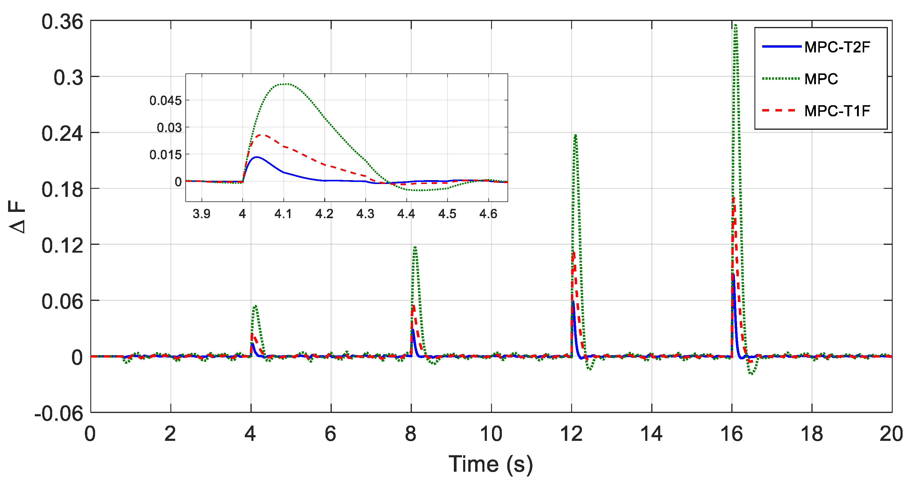
  • In order to damp the frequency fluctuations in the microgrid, a new adaptive MPC controller is used.
  • A powerful type-2 fuzzy tool is used to estimate the parameters of the control system.
  • Uncertainty in all system parameters as well as uncertainty in solar and wind resources is considered.
The article is compiled in the following sections: Section 2: General Structure of Microgrids and Their Control Strategies; Section 3: Model Predictive Control; Section 4: Simulation; Section 5: Conclusions.

2. General Structure of Microgrids and Their Control Strategies

2.1. Microgrid Structure

The studied microgrid structure is shown in Figure 1, which is in a separate state from the main grid. From the upper left corner, there are wind turbines, converters, hydrogen electrolyzers, fuel cells, loads, batteries, flywheels, photovoltaics and diesel generators. They are controlled by converters that connected to the main bus.
For a small signal model of microgrid components to investigate the load-frequency control problem in a microgrid, it is necessary to use small signal models of the renewable energy sources and storage devices (which are linearized around the operating point). The small signal models of each of the microgrid components are as follows:

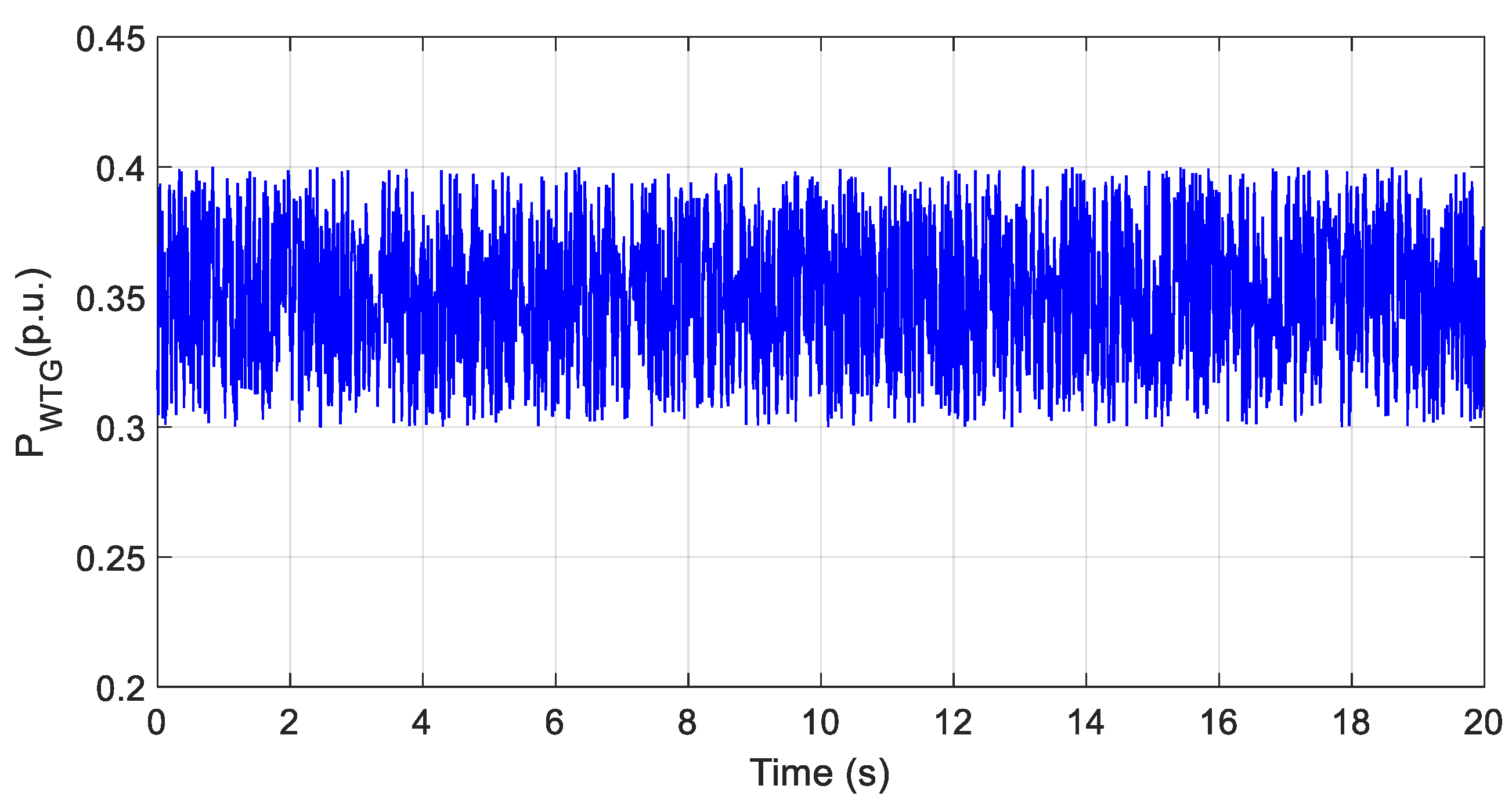
2.1.1. Wind Turbine Generator (WTG)

In the analysis of small signal, the dynamic model of the wind turbine can be determined using Equation (1). Also, Equation (2) expresses its characteristic function.
P W T G ˙ = k a k W T G P W T G T W T G P W T G T W T G
G W T G ( s ) = k a k W T G 1 + s T W T G = P W T G ( s ) P W ( s )
In Equations (1) and (2), k W T G and T W T G are wind turbine and time constants, respectively; k a is the percentage of generated power to the grid, from the microgrid. P W T G is the change in electrical power achieved from a wind turbine, and P W is the Changes in the power of wind. Equation (3) shows the mechanical power obtained from the wind.
P w = 1 2 C p . ρ . A r . V w 3
In Equation (3), C p is the efficiency of the turbine; ρ is air density (kg/m3); A r is the swept area of the blade (m2); and finally, V w is wind speed (m/s).

2.1.2. Photovoltaic (PV)

In the analysis of small signal, the dynamic model of the solar cell can be determined using Equation (4). Also, Equation (5) expresses its characteristic function.
P P V ˙ = k P V T P V P P V T P V
G P V ( s ) = k P V 1 + s T P V = P P V ( s )
In Equations (4) and (5), k P V and T P V are the gain and the time constant of the solar cell, respectively. P P V is the change in the electric power output of the solar cell, and finally, Also, changes in the intensity of solar radiation are indicated by . The electric power output of the solar cell is calculated as follows:
P P V = η S [ 1 0.005 × ( T a + 25 ) ]
In Equation (6), η is the solar cell efficiency, S is the solar cell area, (m2) is the intensity of solar radiation (kw/m2) and Also, the ambient temperature is indicated by T a (°C).

2.1.3. Diesel Generator (DEG)

Diesel generators play a major role in independent hybrid microgrids, so that when the load increases, it is liable for providing part of the power required to reach equilibrium. In the analysis of small signal, the dynamic model of the diesel generator can be determined using Equation (7). Also, Equation (8) expresses its characteristic function.
P D E G ˙ = K D E G P C T D E G K D E G F R T D E G P D E G T D E G
G D E G ( s ) = k D E G 1 + s T D E G = P F R G ( s ) U D E G ( s )
U D E G ( s ) = P C ( s ) F ( s ) R
In Equations (7)–(9), K D E G and T D E G are the gain and time constant of the diesel generator system, respectively; R is the velocity drop coefficient; P D E G is the change in the diesel generator power; P C is the change in the diesel generator control signals; and finally, ∆F is the frequency change.

2.1.4. Electrolyzer (AE)

The electrolyzer provides the hydrogen needed for a fuel cell. The power of the electrolyzer is provided by a part of the power of the wind turbine ( 1 K a ) P W T G . In the analysis of small signal, the dynamic model of the electrolyzer can be determined using Equation (10). Also, Equation (11) expresses its characteristic function.
P A E ˙ = K A E ( 1 K a ) P W T G T A E P A E T A E
G A E ( s ) = k A E 1 + s T A E = P A E ( s ) P t ( s )
  P t ( s ) = ( 1 K t ) P W T G ( s )           ,   K t = 0.6
where K A E and T A E are the gain and electrolyzer time constant, respectively, P A E is the change in the hydrogen produced by the electrolyzer, and P t is the change in the input power to the electrolyzer.

2.1.5. Fuel Cell (FC)

The dynamic model of the fuel cell is described in the small signal analysis with relation (11) and its characteristic function is described in relation (12).
P F C ˙ = K F C P A E T F C P F C T F C
G F C ( s ) = k F C 1 + s T F C = P F C ( s ) P A E ( s )
In Equation (13), K F C and TFC are the gain and time constant of the fuel cell, respectively; P F C is the change in the electrical power output of the fuel cell.

2.1.6. Battery Storage System (BESS) and Flywheel (FESS)

The battery storage system (flywheel) stores the electrical energy received in the form of chemical energy (mechanical). Excess energy in microgrids is stored in batteries and flywheels. By doing this, the lack of energy can be supplied. The dynamic models of the battery and flywheel in small signal analysis are described by Equations (15) and (16), respectively. Additionally, its characteristic functions are described in Equations (17) and (18), respectively.
P B E S S ˙ = K B E S S U B E S S T B E S S P B E S S T B E S S  
P F E S S ˙ = K F E S S U F E S S T F E S S P F E S S T F E S S
G B E S S ( s ) = k B E S S 1 + s T B E S S = P B E S S ( s ) U B E S S ( s )
G F E S S ( s ) = k F E S S 1 + s T F E S S = P F E S S ( s ) U F E S S ( s )
In Equations (15)–(18), k B E S S and T B E S S are the gain and time constant of the battery system, and k F E S S and T F E S S are the gain and time constant of the flywheel system, respectively. The changes in battery power and flywheel power are denoted by P B E S S and P F E S S , respectively. ∆UBESS changes the signal applied to control the battery system and ∆UFESS changes the signal applied to control the flywheel system.

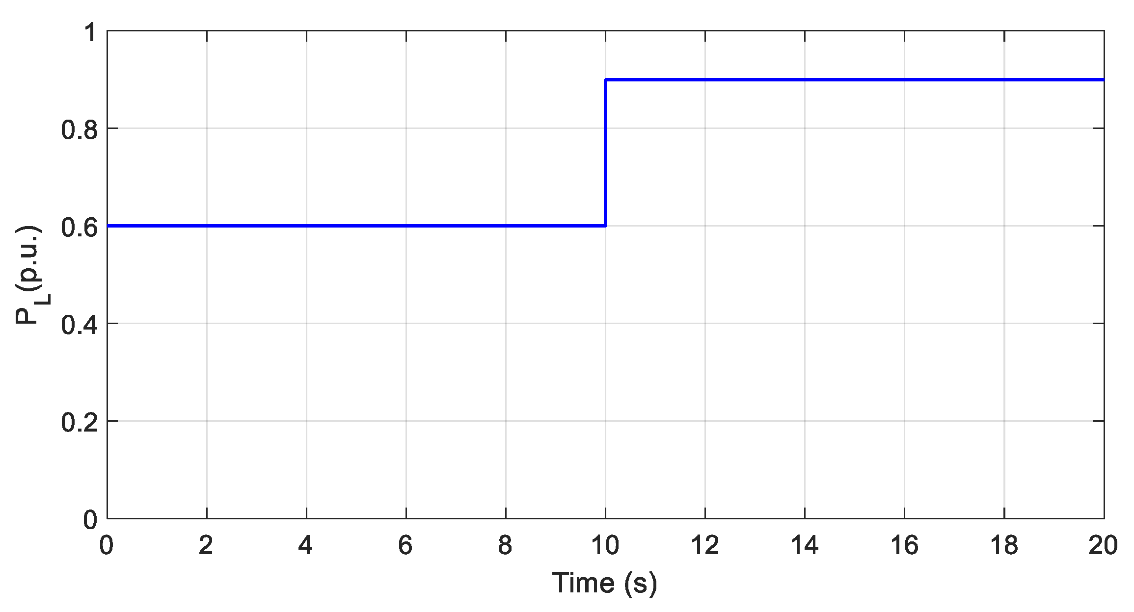
2.1.7. Changes in Frequency and Microgrid Power

If the power delivered to the grid from the microgrid side changes, the frequency will also fluctuate. Equation (19) represents the microgrid dynamic model. This relationship is for small signal analysis.
G S Y S ( s ) = 1 K S Y S ( 1 + s T S Y S ) = 1 2 H s + D = F ( s ) P ( s )
In Equation (19), D is the system damping constant, H is the system inertia constant, F is the system frequency changes, and P is the system power changes. These changes are calculated as follows:
P = P s P L
P s = K t P W T G + P P V + P D E G + P F C + P F E S S + P B E S S
In Equations (20) and (21), P s is the change due to the electrical power of the microgrid sources, and P L is the change in the microgrid load.

2.2. Frequency Control

If there is a disturbance in the microgrid, the frequency changes and causes the power balance to be disturbed. At this stage, the frequency should return to its nominal value with the help of two primary and secondary controllers.
  • Primary Frequency Control (PFC)
Using Equation (22) and according to Figure 2, we can define the primary frequency control of the microgrid that has a diesel generator.
f × 1 R = P ,       f = f f 0 ,       P = P P 0
where R is the drop coefficient.
B.
Secondary Frequency Control (SFC)
The dropped frequency is limited by the primary control loop but still cannot reach its nominal value. For this reason, another control loop (secondary control loop) is used [37]. In this study, MPC tuned by a type-2 fuzzy system is used. Using this method, in the secondary control loop, the frequency can be returned to its nominal value.

3. Model Predictive Control

3.1. General Structure

Model-based predictive controllers have been used in a wide range of applications in various industries such as chemical processes, the petroleum industry and electromechanical systems. Using the model of a system, its future behavior is predicted and controlled. By minimizing the cost function, we can obtain the control signal in this controller. In order for the system output to follow a reference value in the future, the control signal values must be determined correctly. Achieving this goal is possible by minimizing the cost function. Equation (23) shows the cost function, and Equations (24) show the constraints applied on the control signals. Also Equation (25) show the constraints applied on the output signals.
J ( N 1 , N 2 , N u ) = J = N 1 N 2 β ( j ) [ y ( k + j | k ) W ( k + j ) ] 2 + j = 1 N u λ ( j ) [ u ( k + j 1 ) ] 2
u m i n u ( k ) u m a x
y m i n y ( k ) y m a x
In above equation, J ( N 1 , N 2 , N u ) is a cost function and it must be minimized. N 1 and N 2 are the lower and the upper ranges of the prediction window, and N u is the length of the control window (these three parameters are calculated online by the type-2 fuzzy system). The predicted value of the output signal when we are at moment k is denoted by y ( k + j | k ) . W ( k + j ) is the reference output at the moment k + j . The error and control signal weighting coefficients are denoted by β ( j ) and λ ( j ) , respectively (these two parameters are calculated online by the type-2 fuzzy system).

3.2. Predictive Controller Design

If the amount of production of each source or the number of loads in the microgrid changes, the frequency will also change. Microgrids can be divided into controllable and uncontrollable categories. From the controllable category, diesel generators can be mentioned, and from the non-controllable category, wind turbines can be mentioned. When designing the predictive controller, load changes are considered unpredictable disturbances and changes in resource generation are considered predictable disturbances. The state space equations of the predictive control are as follows:
X ˙ = A X + B U + D W Y = C X X = [ F     P D E G       P B E S S       P F E S S ] T U = [ u D E G         u B E S S         u F E S S ] T
A = [ D 2 H 1 2 H 1 2 H 1 2 H K D E G R T D E G 1 T D E G 0 0 0 0 0 0 1 T B E S S 0 0 1 T F E S S ]   ,                               B = [ 0 0 0 K D E G T D E G 0 0 0 0 K B E S S T B E S S 0 0 K F E S S T F E S S ]                 D = [ 1 2 H 0 0 0 ] T ,                                           C = [ 1 0 0 0 ]
where X is the vector of state variables; A is the state space matrix; U is the control vector; B is a matrix of the control coefficients; W is the disturbance vector (uncontrollable input); and finally, D is the matrix of disturbance coefficients.
In the first stage of the proposed method, the changes in power and load resources as well as the microgrid frequency are evaluated and measured; then, in the second stage, the system output prediction and the application of appropriate control signals are conducted. The operation of the control system is as follows:
m i n U J = J = N 1 N 2 W j ( F ( k + j ) ) 2 + i = 1 N u V i ( u D E G ( k + j ) u D E G ( k + j 1 ) ) 2
subject to
u D E G ( k ) = u D E G ( k 1 ) + i = 0 N t δ i F ( k i )
U m i n | u D E G ( k ) u D E G ( k 1 ) | U m a x
W i m i n W j W j m a x
V j m i n V j V j m a x
U = { u D E G ( k ) , u D E G ( k + 1 ) , , u D E G ( k + N u ) }
X ( k + 1 ) = A X   ( k ) + B U   ( k ) + D W   ( k ) Y   ( k ) = C X   ( k )
u B E S S = k B F   ,             u F E S S = k F F
In the above equations, Equation (27) is the objective function, which is arranged in a square programming, and by minimizing it, the set of control signals (Equation (32)) are obtained. Using Equation (26), we can calculate the u D E G signal in each time game. δ i is a numerical coefficient that can be solved by minimizing the problem. The minimum and maximum control signals applied in each stage are expressed in Equation (29). The range of coefficients in the objective function is shown in Equations (30) and (31) (these parameters are calculated online by the type-2 fuzzy system). Equation (33) describes how to calculate state variables at each time step. Equation (34) Indicates the control signals of the energy storage resources The coefficients k B and k F are for the proportional controller (these two parameters are calculated online by the type-2 fuzzy system). The following index can also be calculated to validate the performance of the control systems.
P i n d e x = 0 T | F | 2 d t
Using Equation (33), we can compare the control methods introduced in the simulation section. In addition to damping the microgrid frequency, it must also control and adjust the microgrid voltage level with power source converters as well as the diesel generator excitation system. How to control the voltage in the microgrid is an independent issue and is not presented in this article. Figure 2 shows the general structure of the proposed control system.
As shown in Figure 2, the type-2 fuzzy system calculates the MPC, and the k B and k F coefficients online by processing the F and its values in the past moments, as well as the U D E G , U B E S S and U F E S S signals. The type-2 fuzzy system database can be prepared in two ways: one is to use the information and experience of an expert person (rule-based lookup table), and the other is to extract data by running the system at different work points and to train the system. In this article, the second method is used. The way it works is that first, the closed-loop microgrid system is run many times by changing the amount of parameters, load, resource power, etc., and a rich database is obtained. These data are then used to learn the type-2 fuzzy system (based on a neural network or using evolutionary algorithms). For more information on the type-2 fuzzy system and its equations, see [35,36].

4. Simulation

As stated in Section 3, a variety of renewable energy sources are considered in the simulated microgrid. The parameter values of the renewable energy sources are shown in Table 1.
To evaluate the performance of the proposed control method, the simulation was performed in a MATLAB/Simulink environment. The simulations were performed for three control systems: traditional MPC (the controller coefficients and parameters are fixed); adjustable MPC by the type-1 fuzzy system; and finally, adjustable MPC by the type-2 fuzzy system. The three main challenges of the frequency control system in microgrids are load changes, changes in the power of distributed generation sources and changes in system parameters (due to time lapse and wear, climate change, lack of nonlinear dynamics modeling of the system, etc.). Figure 3 and Figure 4 show the change in solar cell and wind power respectively. Also, Figure 5 shows microgrid load changes.
The simulation was performed in six scenarios.
Scenario 1: In the first scenario, only changes in PV and wind power generation (Figure 3 and Figure 4) were applied. The performances of all three control systems for scenario 1 are shown in Figure 6.
As can be seen from Figure 6, at the moment t = 5   s , when the photovoltaic generating power drops by 0.3 p.u., the frequency also decreases. It can be seen in this figure that the traditional MPC frequency drop is more than twice that of the other two methods.
Scenario 2: In scenario 2, load changes are also added to scenario 1. The performances of the control systems for scenario 2 are shown in Figure 7.
In this scenario, the load increases by 0.3   p . u . at t = 10 s. As can be seen, the frequency change in the T2Fuzzy-MPC method is about 0.15 Hz; in the T1Fuzzy-MPC method, it is about 0.19 Hz; and finally, in the traditional MPC method, it is about 0.38 Hz.
Scenario 3: In this scenario, all power sources’ gains ( K F E S S , K B E S S , K F C , K A E , K P V , K W T G , and K D E G ) increase by 20% of their nominal value at the moment t = 5   s and then decrease from the current value to 20% below the nominal value at the moment t = 15   s . The performances of the control systems for scenario 3 are shown in Figure 8.
Parameter uncertainty is one of the challenges of any control system. All systems, more or less, suffer from this phenomenon due to several reasons such as wear and tear over time, environmental changes, improper use of the system, etc. In microgrids, system parameters change over time. If the control system is not robust to parametric uncertainty, it cannot provide an appropriate response. As can be seen in Figure 8, if the gain parameters of t = 5   s increase by 20% at once (worst possible case in a practical system), the frequency changes in the proposed method are 0.2 Hz, that in the x method is about 0.47 Hz, and that in the z method is about 0.64 Hz. You can also see the performances of all three control systems in the case of gain rates falling to 20% below the nominal value (falling about 33% of the current value) at the moment t = 15   s .
Scenario 4: In this scenario, all time constants of the power sources ( T F E S S , T B E S S , T F C , T A E , T P V , T W T G , and T D E G ) increase by 20% of their nominal value at the moment t = 10   s , then decrease from the current value to 20% below the nominal value at the moment t = 15   s . The performances of the control systems for scenario 4 are shown in Figure 9.
Changes in the time constant parameter in the direction of the horizontal axis (time axis) are more visible. Therefore, a load pulse is applied in three moments t = 5   s , t = 10   s and t = 15   s . At t = 5   s , the time constant parameters have nominal values; for t = 10   s , the time constant parameters are 20% higher than the nominal values; and finally, for t = 15   s , the time constant parameters are 20% less than the nominal value. It is carefully observed in Figure 9 that the oscillation width (system response to pulse load) at t = 10   s is greater than the oscillation width at t = 5   s . Additionally, the oscillation width at t = 15   s is less than the oscillation width at t = 5   s . In other words, any change in time constant parameters, in addition to affecting the width of the oscillation, also affects its height.
Scenario 5: In this scenario, the power system parameters ( 2 H , D ) increase by 20% of their nominal value at the moment t = 5   s and then falls from the current value to 20% below the nominal value at the moment t = 15   s . The performance of the control systems for scenario 5 is shown in Figure 10.
As can be seen in Figure 10, changes in power system parameters also affect frequency changes. Compared to the gain rate changes (Scenario 3, Figure 8), it is observed that frequency changes have occurred to a lesser extent.
Scenario 6: In this scenario, load shedding is applied with four steps (Figure 11). Load shedding is a common practice in the power system. If the frequency cannot return to the nominal value, the operator will have to shed the loads one by one (with priority). The performance of the control systems for scenario 6 is shown in Figure 12.
Figure 11 shows the step reduction in the load at every 4 s (the height of each step is twice the previous step). In the first step, the load is reduced from 1   p . u . to 0.95   p . u . , and in the last step, the load is reduced from 0.65   p . u . to 0.35   p . u . (critical state in a practical system). As can be seen from Figure 12, the self-tuning MPC performance is much better and faster than that of traditional MPC. Additionally, by observing the magnified area (around t = 4   s ), it is seen that the frequency changes in the T2Fuzzy MPC method are about half that of the T1Fuzzy MPC method.

5. Conclusions

In this paper, a new self-tuning MPC method for load frequency control in an islanded microgrid was presented. For automatic adjustment of the MPC parameters, a type-2 fuzzy system was used as a powerful tool in computational intelligence. By learning the dynamics and behavior of microgrids in different operating modes, this tool was able to issue adjustment signals for the control system in the face of load changes, parametric uncertainty, and changes in photovoltaic and wind turbine generating power. In the Simulation section, the proposed method was compared with self-tuning MPC based on a type-1 fuzzy system as well as traditional MPC. The results showed that the proposed method has the best performance in stabilizing the microgrid load frequency, despite the mentioned challenges. As an interesting suggestion to continue this paper, the type-2 fuzzy system can be designed in such a way that, in addition to setting the MPC parameters, it also generates a compensation signal (together with the MPC signal).

Author Contributions

Conceptualization, D.Z., S.S., A.M. (Ardashir Mohammadzadeh) and A.M. (Amir Mosavi); Formal analysis, D.Z., S.S., A.M. (Ardashir Mohammadzadeh) and A.M. (Amir Mosavi); Methodology, D.Z., S.S., A.M. (Ardashir Mohammadzadeh) and A.M. (Amir Mosavi). All authors have read and agreed to the published version of the manuscript.

Funding

This research received no external funding.

Institutional Review Board Statement

Not applicable.

Informed Consent Statement

Not applicable.

Data Availability Statement

Not applicable.

Conflicts of Interest

The authors declare no conflict of interest.

References

  1. Alasali, F.; Salameh, M.; Semrin, A.; Nusair, K.; El-Naily, N.; Holderbaum, W. Optimal Controllers and Configurations of 100% PV and Energy Storage Systems for a Microgrid: The Case Study of a Small Town in Jordan. Sustainability 2022, 14, 8124. [Google Scholar] [CrossRef]
  2. Mohammadi, F.; Mohammadi-ivatloo, B.; Gharehpetian, G.B.; Ali, M.H.; Wei, W.; Erdinç, O.; Shirkhani, M. Robust Control Strategies for Microgrids: A Review. IEEE Syst. J. 2021, 16, 2401–2412. [Google Scholar] [CrossRef]
  3. Iranmehr, H.; Aazami, R.; Tavoosi, J.; Shirkhani, M.; Azizi, A.; Mohammadzadeh, A.; Mosavi, A.H. Modeling the Price of Emergency Power Transmission Lines in The Reserve Market Due to The Influence of Renewable Resources. Front. Energy Res. 2022, 9. [Google Scholar] [CrossRef]
  4. Tavoosi, J.; Shirkhani, M.; Azizi, A.; Din, S.U.; Mohammadzadeh, A.; Mobayen, S. A hybrid approach for fault location in power distributed networks: Impedance-based and machine learning technique. Electr. Power Syst. Res. 2022, 210, 108073. [Google Scholar] [CrossRef]
  5. Wang, H.; Liu, Y.; Fang, J.; He, J.; Tian, Y.; Zhang, H. Emergency sources pre-positioning for resilient restoration of distribution network. Energy Rep. 2020, 6 (Suppl. 9), 1283–1290. [Google Scholar] [CrossRef]
  6. Aazami, R.; Heydari, O.; Tavoosi, J.; Shirkhani, M.; Mohammadzadeh, A.; Mosavi, A. Optimal Control of an Ener-gy-Storage System in a Microgrid for Reducing Wind-Power Fluctuations. Sustainability 2022, 14, 6183. [Google Scholar] [CrossRef]
  7. Li, W.; Zhang, M.; Deng, Y. Consensus-Based Distributed Secondary Frequency Control Method for AC Microgrid Using ADRC Technique. Energies 2022, 15, 3184. [Google Scholar] [CrossRef]
  8. Alayi, R.; Zishan, F.; Seyednouri, S.R.; Kumar, R.; Ahmadi, M.H.; Sharifpur, M. Optimal Load Frequency Control of Island Microgrids via a PID Controller in the Presence of Wind Turbine and PV. Sustainability 2021, 13, 10728. [Google Scholar] [CrossRef]
  9. Kumar, D.; Mathur, H.D.; Bhanot, S.; Bansal, R.C. Modeling and frequency control of community micro-grids under stochastic solar and wind sources. Eng. Sci. Technol. Int. J. 2020, 23, 1084–1099. [Google Scholar] [CrossRef]
  10. Lan, Z.; Wang, J.; Zeng, J.; He, D.; Xiao, F.; Jiang, F. Constant Frequency Control Strategy of Microgrids by Coordinating Energy Router and Energy Storage System. Math. Probl. Eng. 2020, 2020, 4976529. [Google Scholar] [CrossRef]
  11. Al Sumarmad, K.A.; Sulaiman, N.; Wahab, N.I.A.; Hizam, H. Energy Management and Voltage Control in Microgrids Using Artificial Neural Networks, PID, and Fuzzy Logic Controllers. Energies 2022, 15, 303. [Google Scholar] [CrossRef]
  12. Sohrabzadi, E.; Gheisarnejad, M.; Esfahani, Z.; Khooban, M.H. A novel intelligent ultra-local model control-based type-II fuzzy for frequency regulation of multi-microgrids. Trans. Inst. Meas. Control. 2022, 44, 1134–1148. [Google Scholar] [CrossRef]
  13. Huang, H.; Shirkhani, M.; Tavoosi, J.; Mahmoud, O. A New Intelligent Dynamic Control Method for a Class of Stochastic Nonlinear Systems. Mathematics 2022, 10, 1406. [Google Scholar] [CrossRef]
  14. Veronica, A.J.; Kumar, N.S.; Gonzalez-Longatt, F. Design of Load Frequency Control for a Microgrid Using D-partition Method. Int. J. Emerg. Electr. Power Syst. 2020, 21, 20190175. [Google Scholar] [CrossRef]
  15. Latif, A.; Hussain, S.S.; Das, D.C.; Ustun, T.S.; Iqbal, A. A review on fractional order (FO) controllers’ optimization for load frequency stabilization in power networks. Energy Rep. 2021, 7, 4009–4021. [Google Scholar] [CrossRef]
  16. Rafiee, A.; Batmani, Y.; Ahmadi, F.; Bevrani, H. Robust Load-Frequency Control in Islanded Microgrids: Virtual Synchronous Generator Concept and Quantitative Feedback Theory. IEEE Trans. Power Syst. 2021, 36, 5408–5416. [Google Scholar] [CrossRef]
  17. Khokhar, B.; Dahiya, S.; Singh Parmar, K.P. A Robust Cascade Controller for Load Frequency Control of a Standalone Microgrid Incorporating Electric Vehicles. Electr. Power Compon. Syst. 2020, 48, 711–726. [Google Scholar] [CrossRef]
  18. Tripathi, S.K.; Singh, V.P.; Pandey, A.S. Robust Load Frequency Control of Interconnected Power System in Smart Grid. IETE J. Res. 2021. [Google Scholar] [CrossRef]
  19. Anuradhika, K.; Dash, P. Genetic Algorithm-Based Load Frequency Control of a Grid-Connected Microgrid in Presence of Electric Vehicles. In Sustainable Energy and Technological Advancements; Panda, G., Naayagi, R.T., Mishra, S., Eds.; Advances in Sustainability Science and Technology; Springer: Singapore, 2022. [Google Scholar] [CrossRef]
  20. Ramlal, C.J.; Singh, A.; Rocke, S. Repetitive Learning Frequency Control for Energy Intensive Corporate Microgrids subject to Cyclic Batch Loads. In Proceedings of the 2020 IEEE PES Innovative Smart Grid Technologies Europe (ISGT-Europe), The Hague, The Netherlands, 26–28 October 2020; pp. 349–353. [Google Scholar] [CrossRef]
  21. Saleh-Ahmadi, A.; Moattari, M.; Gahedi, A.; Pouresmaeil, E. Droop Method Development for Microgrids Control Considering Higher Order Sliding Mode Control Approach and Feeder Impedance Variation. Appl. Sci. 2021, 11, 967. [Google Scholar] [CrossRef]
  22. Keyvani, B.; Fani, B.; Karimi, H.; Moazzami, M.; Shahgholian, G. Improved Droop Control Method for Reactive Power Sharing in Autonomous Microgrids. J. Renew. Energy Environ. 2022, 9, 1–9. [Google Scholar] [CrossRef]
  23. Qiao, S.; Liu, X.; Xiao, G.; Ge, S.S. Observer-Based Sliding Mode Load Frequency Control of Power Systems under Deception Attack. Complexity 2021, 2021, 8092206. [Google Scholar] [CrossRef]
  24. Mishra, D.; Nayak, P.C.; Prusty, R.C. PSO optimized PIDF controller for Load-frequency control of A.C Multi-Islanded-Micro grid system. In Proceedings of the International Conference on Renewable Energy Integration into Smart Grids: A Multidisciplinary Approach to Technology Modelling and Simulation (ICREISG), Bhubaneswar, India, 14–15 February 2020; pp. 116–121. [Google Scholar] [CrossRef]
  25. El-Fergany, A.A.; El-Hameed, M.A. Efficient frequency controllers for autonomous two-area hybrid microgrid system using social-spider optimiser. IET Gener. Transm. Distrib. 2017, 11, 637–648. [Google Scholar] [CrossRef]
  26. Ibrahim, A.N.A.A.; Shafei, M.A.R.; Ibrahim, D.K. Linearized biogeography based optimization tuned PID-P controller for load frequency control of interconnected power system. In Proceedings of the Nineteenth International Middle East Power Systems Conference (MEPCON), Cairo, Egypt, 19–21 December 2017; pp. 1081–1087. [Google Scholar] [CrossRef]
  27. Shafei, M.A.R.; Ibrahim, D.K.; Bahaa, M. Application of PSO tuned fuzzy logic controller for LFC of two-area power system with redox flow battery and PV solar park. Ain Shams Eng. J. 2022, 13, 101710. [Google Scholar] [CrossRef]
  28. Jeyalakshmi, V.; Subburaj, P. PSO-scaled fuzzy logic to load frequency control in hydrothermal power system. Soft Comput. 2016, 20, 2577–2594. [Google Scholar] [CrossRef]
  29. Rawat, S.; Jha, B.; Panda, M.K.; Kanti, J. Interval Type-2 Fuzzy Logic Control-Based Frequency Control of Hybrid Power System Using DMGS of PI Controller. Appl. Sci. 2021, 11, 10217. [Google Scholar] [CrossRef]
  30. Sahu, P.C.; Mishra, S.; Prusty, R.C.; Panda, S. Improved-salp swarm optimized type-II fuzzy controller in load frequency control of multi area islanded AC microgrid. Sustain. Energy Grids Netw. 2018, 16, 380–392. [Google Scholar] [CrossRef]
  31. Li, L.; Li, H.; Tseng, M.-L.; Feng, H.; Chiu, A.S.F. Renewable Energy System on Frequency Stability Control Strategy Using Virtual Synchronous Generator. Symmetry 2020, 12, 1697. [Google Scholar] [CrossRef]
  32. Cao, Y.; Mohammadzadeh, A.; Tavoosi, J.; Mobayen, S.; Safdar, R.; Fekih, A. A new predictive energy management system: Deep learned type-2 fuzzy system based on singular value decommission. Energy Rep. 2022, 8, 722–734. [Google Scholar] [CrossRef]
  33. Garcia-Torres, F.; Vazquez, S.; Moreno-Garcia, I.M.; Gil-de-Castro, A.; Roncero-Sanchez, P.; Moreno-Munoz, A. Microgrids Power Quality Enhancement Using Model Predictive Control. Electronics 2021, 10, 328. [Google Scholar] [CrossRef]
  34. Tavoosi, J.; Shirkhani, M.; Abdali, A.; Mohammadzadeh, A.; Nazari, M.; Mobayen, S.; Asad, J.H.; Bartoszewicz, A. A New General Type-2 Fuzzy Predictive Scheme for PID Tuning. Appl. Sci. 2021, 11, 10392. [Google Scholar] [CrossRef]
  35. Hasan, N.; Alsaidan, I.; Sajid, M.; Khatoon, S.; Farooq, S. Hybrid MPC-Based Automatic Generation Control for Dominant Wind Energy Penetrated Multisource Power System. Model. Simul. Eng. 2022, 2020, 5526827. [Google Scholar] [CrossRef]
  36. Sayedi, I.; Fatehi, M.H.; Simab, M. Optimal Load Distribution in DG Sources Using Model Predictive Control and the State Feedback Controller for Switching Control. Int. Trans. Electr. Energy Syst. 2022, 2022, 5423532. [Google Scholar] [CrossRef]
  37. Kayalvizhi, S.; Kumar, D.M.V. Load Frequency Control of an Isolated Micro Grid Using Fuzzy Adaptive Model Predictive Control. IEEE Access 2017, 5, 16241–16251. [Google Scholar] [CrossRef]
Figure 1. Microgrid schematic.
Sustainability 14 11772 g001
Figure 2. The proposed self-tuning MPC based on a type-2 fuzzy system.
Sustainability 14 11772 g002
Figure 3. Solar cell power changes.
Sustainability 14 11772 g003
Figure 4. Wind turbine power changes.
Sustainability 14 11772 g004
Figure 5. Microgrid load changes.
Sustainability 14 11772 g005
Figure 6. The performance of all three control systems for scenario 1.
Sustainability 14 11772 g006
Figure 7. The performances of all three control systems for scenario 2.
Sustainability 14 11772 g007
Figure 8. The performances of all three control systems for scenario 3.
Sustainability 14 11772 g008
Figure 9. The performances of all three control systems for scenario 4.
Sustainability 14 11772 g009
Figure 10. The performance of all three control systems for scenario 5.
Sustainability 14 11772 g010
Figure 11. Load shedding.
Sustainability 14 11772 g011
Figure 12. The performance of all three control systems for scenario 6.
Sustainability 14 11772 g012
Table 1. Microgrid power sources parameters values.
ParameterValueParameterValue
D (p.u./Hz)0.012 K t 0.6
T F E S S   ( s ) 0.1 K F E S S −0.01
T B E S S   ( s ) 0.1 K B E S S −0.003
T F C   ( s ) 4 K F C 0.01
T A E   ( s ) 0.5 K A E 0.002
T P V (s)1.8 K P V 1
T W T G   ( s ) 1.5 K W T G 1
T D E G   ( s ) 2 K D E G 0.003
H (p.u.s) 0.084 R (Hz/p.u.)3
Publisher’s Note: MDPI stays neutral with regard to jurisdictional claims in published maps and institutional affiliations.

